https://doi.org/10.5194/gmd-10-2471-2017 © Author(s) 2017. This work is distributed under the Creative Commons Attribution 3.0 License.
An emission module for ICON-ART 2.0: implementation and
simulations of acetone
Michael Weimer1,2, Jennifer Schröter2, Johannes Eckstein2, Konrad Deetz2, Marco Neumaier2, Garlich Fischbeck2, Lu Hu3, Dylan B. Millet4, Daniel Rieger2, Heike Vogel2, Bernhard Vogel2, Thomas Reddmann2, Oliver Kirner1, Roland Ruhnke2, and Peter Braesicke2
1Steinbuch Centre for Computing, Karlsruhe Institute of Technology, 76344 Eggenstein-Leopoldshafen, Germany 2Institute of Meteorology and Climate Research, Karlsruhe Institute of Technology,
76344 Eggenstein-Leopoldshafen, Germany
3Department of Chemistry and Biochemistry, University of Montana, Missoula, MT 59812, USA 4Department of Soil, Water, and Climate, University of Minnesota, Saint Paul, MN 55108, USA
Correspondence to:Michael Weimer ([email protected]) Received: 7 October 2016 – Discussion started: 24 October 2016
Revised: 4 May 2017 – Accepted: 30 May 2017 – Published: 29 June 2017
Abstract.We present a recently developed emission module for the ICON (ICOsahedral Non-hydrostatic)-ART (Aerosols and Reactive Trace gases) modelling framework. The emis-sion module processes external flux data sets and increments the tracer volume mixing ratios in the boundary layer accord-ingly.
The performance of the emission module is illustrated with simulations of acetone, using a simplified chemical depletion mechanism based on a reaction with OH and photolysis only. In our model setup, we calculate a tropospheric acetone life-time of 33 days, which is in good agreement with the liter-ature. We compare our results with ground-based as well as with airborne IAGOS-CARIBIC measurements in the upper troposphere and lowermost stratosphere (UTLS) in terms of phase and amplitude of the annual cycle. In all our ICON-ART simulations the general seasonal variability is well rep-resented but uncertainties remain concerning the magnitude of the acetone mixing ratio in the UTLS region.
In addition, the module for online calculations of biogenic emissions (MEGAN2.1) is implemented in ICON-ART and can replace the offline biogenic emission data sets. In a sen-sitivity study we show how different parametrisations of the leaf area index (LAI) change the emission fluxes calculated by MEGAN2.1 and demonstrate the importance of an ade-quate treatment of the LAI within MEGAN2.1.
We conclude that the emission module performs well with offline and online emission fluxes and allows the simulation of the annual cycles of emissions-dominated substances.
1 Introduction
Many trace gases (called tracers hereafter) are emitted into the atmosphere by sources located at the Earth’s surface. Es-pecially for volatile organic compounds (VOCs), natural and anthropogenic emissions as well as secondary production from emitted precursor compounds are major atmospheric sources (e.g. Blake and Blake, 2002; Atkinson and Arey, 2003).
module (Keller et al., 2014). Emissions in higher altitudes are brought into GEOS-Chem as a tendency in the respec-tive height of the emissions. The MESSy interface (Jöckel et al., 2005) incorporated, for example, in the EMAC model (EMAC: ECHAM/MESSy Atmospheric Chemistry; Jöckel et al., 2006) gives the possibility to choose the used method for including emissions into the model – either emissions are prescribed as flux condition as described above or the increase of the tracer mixing ratio is calculated and added to the tracer (Kerkweg et al., 2006). The latter method is also used for the MACC reanalysis (Monitoring Atmospheric Composition and Climate; Inness et al., 2013) and in the cou-pled limited-area model COSMO-ART (COSMO: COnsor-tium for SMall-scale MOdelling, ART: Aerosols and Reac-tive Trace Gases; Vogel et al., 2009).
Recent work also includes the development of chemistry– climate models on icosahedral grids (Suzuki et al., 2008; El-bern et al., 2010; Niwa et al., 2011; Goto et al., 2015; Rieger et al., 2015). The ICOsahedral Non-hydrostatic modelling framework (ICON) has been designed for the simultaneous usage for numerical weather prediction and climate simula-tions (Zängl et al., 2015). It includes the possibility of lo-cal grid refinement (nests) with two-way interaction. Due to its good scaling properties ICON is applicable on high-performance computers of the next generation.
In the previous version of the coupled chemistry cli-mate modelling framework ICON-ART, only emissions of aerosols are considered (ART: Aerosols and Reactive Trace gases; Rieger et al., 2015). A module accounting for trace gas emissions has not existed so far.
Here we present a module for including emissions from external data sources in ICON-ART which is independent of the temporal resolution of the underlying emission data. This module reads emission mass fluxes from data sets, remapped to the unstructured ICON grid, and interpolates them to the ICON-ART simulation time. After conversion to volume mixing ratio (VMR) the emissions are added to the tracer VMR in ICON-ART in the lowest model layers. This num-ber is specified by the user.
In addition, the Model of Emissions of Gases and Aerosols from Nature (MEGAN2.1; Guenther et al., 2012) as imple-mented in ICON-ART is presented. This model calculates biogenic emissions of VOCs online, i.e. dependent on the current state of the atmosphere.
We also describe a new simplified mechanism for deple-tion of trace gases due to reacdeple-tion with OH, the main tro-pospheric sink for most VOCs (Blake and Blake, 2002). In addition, this mechanism includes photolysis of the species and allows the space- and time-dependent calculation of the tracers’ loss rate. Thus, these new developments now allow the investigation of VOCs with ICON-ART.
Several VOCs act as precursors of OH and HO2(=HOx) radicals particularly in the dryer upper troposphere and low-ermost stratosphere (UTLS) (Folkins and Chatfield, 2000). HOx can deplete ozone so that VOCs have climatic impact
in the UTLS region (e.g. Neumaier et al., 2014). In this study, we will focus on the influence of acetone which is together with methanol one of the most abundant VOC in the UTLS region. Mixing ratios of 300–2000 pptv (1 pptv=
10−12mol mol−1) have been observed in the Northern Hemi-sphere mid-latitudes (Singh et al., 1995; Jaeglé et al., 1998; Heikes et al., 2002; Sprung and Zahn, 2010; Elias et al., 2011; Neumaier et al., 2014).
This study is organised as follows: in Sect. 2 the model ICON with its ART extension is described followed by the description of the emission module in Sect. 3. Then, the sim-plified mechanism for VOC depletion is introduced (Sect. 4). After a description of the used measurements of acetone and the simulations for this study in Sects. 5 and 6, the results are presented in Sect. 7 followed by conclusions and an outlook (Sect. 8).
2 The ICON model with its ART extension
In this section, we briefly describe the ICON model (Sect. 2.1) and its ART extension (Sect. 2.2). More detailed descriptions can be found in Zängl et al. (2015) and Rieger et al. (2015), respectively.
2.1 The ICON model
ICON is a non-hydrostatic atmospheric model developed with the aim of providing a global model for both weather and climate (Wan et al., 2013; Zängl et al., 2015). Since January 2016, it is operationally used for global numerical weather prediction at the German Weather Service (DWD). In July 2016, ICON also replaced the limited area model COSMO-EU (Baldauf et al., 2011) by a nested area over Eu-rope.
Horizontal discretisation is performed on an icosahedral– triangular C grid. In contrast to the regular latitude–longitude grid, this is an unstructured grid where the grid points are saved as one-dimensional arrays.
In this study, we use the same resolution notation as intro-duced by Zängl et al. (2015): RnBkwithnandkas indicators for root division and bisections, respectively. Usual resolu-tions and the corresponding global number of grid cells are shown in Table 1.
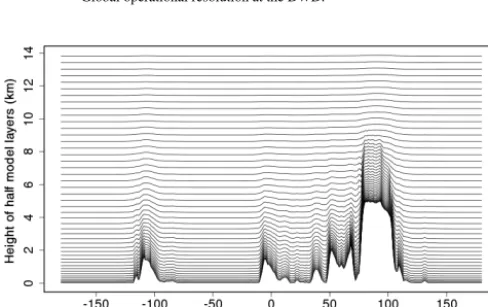
In the vertical, generalised smooth-level coordinates as de-scribed by Leuenberger et al. (2010) are used (see Fig. 1).
Tracers in ICON are transported by solving the continu-ity equation of mass for each tracer discretised with a time-split method: finite volume method is used in the vertical, whereas a simplified flux-form semi-Lagrangian method is used for horizontal transport (Miura, 2007; Lauritzen et al., 2011; Rieger et al., 2015).
Table 1.Examples of ICON resolutions with characteristic length
1x and total number of cells (from Zängl et al., 2015). Char-acteristic length and number of cells are calculated according to
1x=√π/5R/(n2k)andnc=20n24k(R=Earth’s radius andn andkas ICON resolution indicators). The grid number denotes the official ICON grid numberafor the grid configuration used in this study, rotated by 36◦aroundzaxis.
Resolution 1x Number Grid (in km) of cells number
R2B04 157.8 20 480 0012 R2B05 78.9 81 920 0014 R2B06 39.5 327 680 0016 R2B07 19.7 1 310 720 0018 R3B07b 13.9 2 949 120 0022
ahttp://icon-downloads.zmaw.de/dwd_grids.xml
(last access: 3 May 2017).
bGlobal operational resolution at the DWD.
Figure 1.Height of the lowest 46 ICON model layers at 33◦N in the configuration with 90 total model layers.
COSMO (Doms and Schättler, 2004) and described in the technical documentation as part of the ICON source code (Seifert, 2010).
The tropopause height will play an important role in this study. In our simulations, it is calculated by ICON routines according to the thermal definition of World Meteorological Organization (WMO).
2.2 The ART module
The ART module for ICON is currently under development with the following aims (Rieger et al., 2015):
– treatment of aerosols and gas-phase species in global modelling;
– gas-phase and heterogeneous chemistry;
– investigation of the feedbacks between aerosols, trace gases and the state of the atmosphere
Tracers in ICON-ART are transported and diffused in the same way as the internal ICON tracers like water vapour. The ICON-ART tracers used in this study include methane (CH4), carbon monoxide (CO), propane (C3H8) and acetone
(CH3C(O)CH3).
Chemical reactions are calculated according to the follow-ing equation:
∂ρψˆi
∂t = −Ai+Pi−Li+Ei, (1)
whereρ,ψi,Ai andPi are Reynolds-averaged air density, partial density fraction, advection and chemical production of the tracer i, respectively. The hat over ψ denotes the barycentric average.
Ei andLi are emission and loss rate of traceri, respec-tively. In version 1.0 of ICON-ART (Rieger et al., 2015), no general algorithm for includingEiwas included and the life-time and thereforeLi was assumed to be globally constant. In version 2.0 used here, we added a module for emissions (see Sect. 3) and a simplified OH chemistry for calculation of the loss rate (see Sect. 4).
Additionally, we implemented the predictor-corrector method according to Seinfeld and Pandis (2012, pp. 1125– 1126) to solve Eq. (1) for tracer depletion via reaction with OH. This method is more accurate than that described by Rieger et al. (2015). A detailed description of the predictor-corrector method can be found in Appendix A.
3 The emission module in ICON-ART
We have included modules for offline and online calculation of emissions in ICON-ART. Both approaches are described in this section. In Sect. 3.1, we demonstrate our method to read and treat offline emissions, whereas the description of the MEGAN2.1 model for online calculation of biogenic emissions in the configuration for ICON-ART follows in Sect. 3.2.
In order to follow the process splitting concept of ICON (Rieger et al., 2015) and to be compatible with ICON for both numerical weather prediction and climate projections the emission mass flux densities are converted to volume mixing ratio and added to the tracer volume mixing ratios.
We also perform a sensitivity study by including the emis-sions as lower boundary condition in the vertical turbulent diffusion scheme of ICON which can be found in the sup-plement of the paper. In this figure, we demonstrate that the method used in this study (see Sect. 3.1.3) and the method us-ing the turbulent diffusion are equivalent if the emissions are included into the lowermost model layer (nlev,emi=1). This
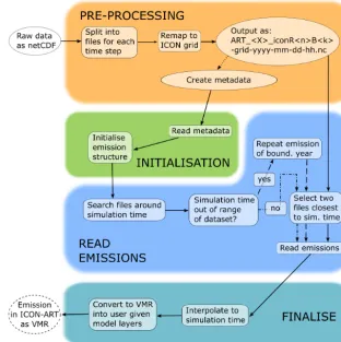
Figure 2.Flow chart of the process from the external netCDF emission data with regular grid and emission data as mass flux density to the emission as VMR in ICON-ART. The process can be separated into four steps: pre-processing, initialisation, read emissions and finalising the module. Pre-processing before the run of ICON-ART is necessary, whereas the other processes are included in ICON-ART. Ellipses depict files while rectangles stand for processes. The different arrow lines illustrate either the interaction with the remapped netCDF data set which has to be performed by the user in the pre-processing step (dotted), the “no” path (dotted and dashed) or the “yes” path (dashed).
3.1 Offline emissions
Offline emissions in ICON-ART are calculated with a new module for including emissions from external data sources which is described in the following. The process can be sep-arated into four steps (see Fig. 2): pre-processing, initialisa-tion, reading and finalisation.
Pre-processing (Sect. 3.1.1) is required before the model run and includes horizontal interpolation of the input data to the ICON grid as well as preparation of meta-information of the data set which is committed to the module during initial-isation.
The other steps are performed automatically during run-time of the model. In the step for reading emission (Sect. 3.1.2), the closest emission dates are searched and the emissions are interpolated to the current simulation time of ICON-ART. Finally, the temporally interpolated emission mass flux density is converted to VMR and added to the tracer VMR in the lowest model layers specified by the user (Sect. 3.1.3).
In addition, we briefly describe the offline emission inven-tories used for this study (Sect. 3.1.4) and demonstrate the performance of the module (see Sect. 3.1.5).
3.1.1 Pre-processing of the input data and initialisation of the module
Due to the unstructured icosahedral grid of ICON (see Sect. 2.1), the usually structured latitude–longitude grid of emission data sets has to be interpolated to the ICON grid. This is managed by tools provided by the DWD called the DWD ICON tools (Prill, 2016). In general, emissions are spatially highly variable. Therefore, the nearest-neighbour interpolation method is applied which reasonably captures the spatial variability of the emissions. This method also con-serves the total emission fluxes reasonably with a maximum deviation of 1 % in the case of R2B04 and a less deviation for the other resolutions of Table 1 (not shown).
emission data have to be split into separate files according to their validity time.
The files to be read by the emission module have to follow the general ICON-ART name convention:
ART_<X>_iconR<n>B<k >-grid-yyyy-mm-dd-hh_<grid-num>.nc,
where<X>characterises the three character abbreviation of the emission type (see Table 2), and <n> and <k> are the ICON resolution indicators in the same format as in Table 1. Additionally, the date of the emissions and the grid number (see Table 1) are part of the name structure. The maximum temporal resolution of the data set is hourly and every file can include emission data of more than one species.
Emission mass flux densities in units of kg m−2s−1 are required in the raw data as the values are automatically con-verted to VMR after the reading process; see Sect. 3.1.3. The controlling LaTeX table and
“first_and_last_date.txt”
Some meta-information has to be committed to the module, e.g. about the data set’s location on the disk and the variable name in the remapped netCDF file for each emission data set and each tracer in ICON-ART. These metadata are controlled by a LaTeX table (see Fig. 3).
In the simplest form, each tracer in the LaTeX table is rep-resented by one line (see tracer CO in Fig. 3). This line con-tains the tracer name (column 1), the number of emission types to be considered (column 2) and the standard value as mass flux density (column 3). The standard value is taken into account only if the number of emission types is zero. Then it is used as the globally applied emission mass flux density. Otherwise one line per emission type follows with empty first column, each giving the following:
– column 2: emission type as integer (see Table 2); – column 3: number of dimensions of the emission data
in the file without the time dimension: 2 or 3, for two-or three-dimensional data;
– column 4: number of lowest model layers into which the emissions shall be included;
– column 5: variable name in the netCDF files; – column 6: full path to the netCDF files.
In the example of Fig. 3, no emission data sets are consid-ered for CO. Since the standard emission value is set to zero as well, no emissions are computed for CO at all. For ace-tone, offline and online emissions have to be considered. The anthropogenic (type is set to 10; see Table 2) and biomass burning data set (type 12) are both two-dimensional emis-sions to be included in one (i.e. the lowest) model layer and with the variable name “acetone” in the netCDF files.
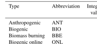
Table 2.Notation of the abbreviations used for different types of emissions denoted as X in the name structure of the files together with the corresponding integer value used in ICON-ART.
Type Abbreviation Integer value
Anthropogenic ANT 10
Biogenic BIO 11
Biomass burning BBE 12 Biogenic online ONL 13
Biogenic emissions in this example are calculated online (type 13). They are also added to the lowest model layer. The path for online emissions refers to the data set of plant func-tional types (see Sect. 3.2).
If the simulation time exceeds the range of the data set the boundary year is repeated as long as necessary (see Fig. 2 in the “read emission” step). That is why the boundary dates of the data set also have to be committed to the module. For this, the ASCII file “first_and_last_date.txt” placed in the same folder as the data set is used containing the first and the last date of the data set in the ICON date format in separate lines as shown in Fig. 4.
3.1.2 Reading emissions
The first task of the module during runtime is to find the two dates closest to the simulation time where emissions are available in the data set. For this, one hour is successively added to or subtracted from the simulation time until a file at that date is found. The next file is searched only if the simu-lation time exceeds the date of the later emission file.
Apart from limits of the temporal resolution, no further assumptions of the data set’s temporal resolution have to be made. Missing files or variable temporal resolution of the data are possible and taken care of by the model. As men-tioned in Sect. 3.1.1, the lower limit of the temporal resolu-tion is hourly. ICON-ART aborts when no file is found before or after 105h (about 11 years) with a corresponding error message.
3.1.3 Time interpolation of the emissions and conversion to VMR
The maximum temporal resolution of the data is hourly (see Sect. 3.1.1) but the model time steps in ICON-ART are in the order of minutes for resolution R2B04 or below for higher resolutions. Therefore, the emission data are linearly inter-polated to the simulation time.
Figure 3.Sample extract of a LaTeX table committing emission metadata to the module. Please note that the header lines are cut. For details of the table content see text.
Figure 4. Content of “first_and_last_date.txt”. It commits the boundary dates of the data set to the module with first date of data set in the first line and last date in the second one. Here, an exam-ple is given for the inventory MEGAN-MACC (see Sect. 3.1.4 for further information).
(moist) airnair: 1Xemi,i=
1ni
nair
. (2)
The moles of the emission are calculated as the emission mass flux densityEi multiplied by the advective model time step1t and the base areaAof the grid box and divided by the molar mass of the speciesMi:
1ni=
EiA 1t
Mi
. (3)
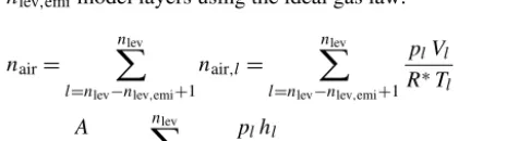
The emission flux can be included into one or more lowest model layers to be specified in the LaTeX table; see Fig. 3. In the following, we will refer to this number asnlev,emi. The
total number of model layers is stated asnlev. In ICON, the lowest model layer has the highest index so that the index of the lowest model layer isl=nlev. For calculating the number of moles of the air we sum up the moles of air of the lowest
nlev,emimodel layers using the ideal gas law:
nair=
nlev
X
l=nlev−nlev,emi+1
nair,l=
nlev
X
l=nlev−nlev,emi+1
plVl
R∗T l
= A
R∗
nlev
X
l=nlev−nlev,emi+1
plhl
Tl
. (4)
Accordingly,pl,Tl,hl andR∗stand for pressure, temper-ature and geometric height of the grid box and the universal gas constant, respectively.
With Eqs. (3) and (4) the VMR tendency of the emission dXemi,i/dt, which is added to the tracer, is calculated accord-ing to
dXemi,i dt ≈
1ni
nair1t
=EiR
∗
Mi
nlev
X
l=nlev−nlev,emi+1
plhl
Tl
−1
. (5)
This method conserves mass of the emission since the cal-culated moles of the emission1ni are independent of the choice ofnlev,emi and therefore do not change if nlev,emi is
increased. The emissions are just distributed in a larger col-umn.
To investigate the differences in changes of nlev,emi
we perform sensitivity simulations of acetone by varying
nlev,emi between 1 and 12. These simulations are based on
constL(megan-offl); see Sect. 6. In Fig. 5, profiles of the ace-tone VMR are shown for the different choices ofnlev,emi.
In the case of nlev,emi=1, no emissions are included in
the layers above in contrast tonlev,emi>1. For larger values
ofnlev,emithe VMR in the lowermost model layer decreases
subsequently since the emissions are distributed into a larger column.
Above the specified emission height, all profiles converge each other and above around 750 hPa the influence of varying
nlev,emiis negligible. Because of our aim to simulate acetone
in the UTLS region, the choice ofnlev,emi should make no
difference. That is why we simply selectnlev,emi=1 for all
used offline emissions. 3.1.4 Emission inventories
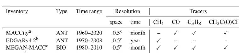
The emission data for the tracers used in this study can be downloaded from the database of Emissions of atmospheric Compounds & Compilation of Ancillary Data (ECCAD, http://eccad.sedoo.fr1). The inventories used for this study are MACCity, EDGARv4.2, MEGAN-MACC and GFED3 and will be described briefly in the following paragraphs. The emission inventories are chosen according to length and tem-poral resolution of the data. A summary of the technical de-tails of each used emission inventory is shown in Table 3. This table also shows which inventory is used for which tracer.
Figure 5.Profiles of the acetone VMR fornlev,emi=1 (emission height of 20 m above ground, black thick) and 2 to 12 (emission height of 65 to∼1500 m above ground, green thin lines) spatially averaged over the Amazon region in Brazil on 29 February 2004, about two months after initialisation. In the right panel, the pressure range is reduced and the average height of the 12 lowest model layers are illustrated by the dashed horizontal lines.
Table 3.Technical details of the emission inventories from ECCAD for tracers in ICON-ART. For abbreviations of the emission types, see Table 2.
Inventory Type Time range Resolution Tracers
space time CH4 CO C3H8 CH3C(O)CH3
MACCitya ANT 1960–2020 0.5◦ month – X X X EDGARv4.2b ANT 1970–2008 0.5◦ year X – – – MEGAN-MACCc BIO 1980–2010 0.5◦ month X X X X
GFED3d BBE 1997–2010 0.5◦ month X X X X
aLamarque et al. (2010), Diehl et al. (2012), Granier et al. (2011) and van der Werf et al. (2006); bJanssens-Maenhout et al. (2011, 2013);cSindelarova et al. (2014);dvan der Werf et al. (2010).
The inventory MACCity includes monthly anthropogenic emissions (Granier et al., 2011). They are taken from the his-torical monthly data set of Atmospheric Chemistry and Cli-mate Model Intercomparison Project (ACCMIP), described by Lamarque et al. (2010), and the Representative Concen-tration Pathways 8.5 (RCP8.5) emission scenario.
In the anthropogenic inventory Emissions Database for Global Atmospheric Research version 4.2 (EDGARv4.2; Janssens-Maenhout et al., 2011, 2013) emissions are calcu-lated with a country-sector method based on emission fac-tors and more than 50 categories of anthropogenic emis-sion sources (for more information see Olivier and Janssens-Maenhout, 2015).
For the inventory MEGAN-MACC (Sindelarova et al., 2014), monthly mean biogenic emissions are calculated with MEGAN2.1 and the same 15 plant functional types as in our configuration (see Sect. 3.2). Meteorological fields are taken from the Goddard Earth Observing System (GEOS) and
as-similated to model space. The leaf area index is derived from MODIS retrievals.
Biomass burning emissions in the inventory called Global Fire Emissions Database version 3 (GFED3; van der Werf et al., 2010) are calculated with a modified version of the Carnegie Ames Stanford Approach model (CASA; Potter et al., 1993; Field et al., 1995; Randerson et al., 1996). Sev-eral fire emission types are derived from satellite data and combined for calculating the carbon emission fluxes on a monthly basis in each grid cell. The emission fluxes for the substances are calculated using emission factors depending on the type of fire.
3.1.5 Performance of the offline module
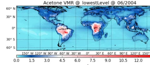
We demonstrate the performance of the module by including offline emissions for acetone as described in Table 3. Fig-ure 6 shows the monthly mean acetone VMR in the lowest model layer for June 2004 in the OH-chem(megan-offl) sim-ulation; see Sect. 6. As biogenic emissions dominate the ace-tone emissions, the maximum values in the aceace-tone VMR occur over central Africa and South America, where the bio-genic emissions of the inventory MEGAN-MACC also are maximised (not shown).
3.2 Online biogenic emissions: MEGAN2.1
To account for the influence of temperature, vegetation and photosynthetically active radiation (PAR) on the emissions of acetone, the Model of Emissions of Gases and Aerosols from Nature version 2.1 (MEGAN2.1, MEGAN-Online hereafter) (Guenther et al., 2012) is implemented into ICON-ART. In contrast to the external acetone data sets (here MEGAN-MACC) which are given as monthly mean values, the on-line calculation of acetone emissions within Guenther et al. (2012) allows to account for the current conditions in me-teorology (especially the diurnal cycle) and vegetation. The parametrisation of biogenic emissions including acetone is described in detail in Guenther et al. (2012), therefore we present here only the main concept of the parametrisation, the changes we have made and the input provided for MEGAN-Online.
MEGAN-Online estimates the biogenic emission mass flux density E in µg m−2h−1 of the compound class c via the following equation:
Ec=γc X
j
c,jχj, (6)
wherec,jis the emission factor depending on the vegetation typejwith the fractional grid box coverageχj. The emission activity factorγcaccounts for environmental and phenologi-cal conditions which affect the emissions.
MEGAN-Online includes 19 compound classes but the study on hand will focus on acetone (c=15). Guenther et al. (2012) consider the emission affecting processes due to light, temperature, leaf age, soil moisture, leaf area index (LAI) and CO2inhibition. The implementation in ICON-ART only
accounts for the emission responses from light, temperature, LAI and leaf age.
The light is provided by ICON-ART as photosynthetically active radiation (PAR) and temperature in the lowest model layer is a standard meteorological variable of ICON-ART. The LAI is based on external parameters read during ini-tialisation of ICON-ART. The leaf age considers the frac-tion of new (FNEW), growing (FGRO), mature (FMAT) and senescing (FSEN) leaves. Due to missing information about the global distribution of these four leaf types, we assumed a uniform distribution. In addition to the standard LAI we
Figure 6.Monthly mean acetone volume mixing ratio in the lowest model layer (layer 90, height of about 20 m above surface) for June 2004, 6 months after initialisation of the OH-chem(megan-offl) sim-ulation (see Sect. 6).
have included the parametrisation of Dai et al. (2004) to de-rive LAIsun, the LAI that is lit by sun and relevant for the
emissions of biogenic VOCs: LAIsun=
1
kb
(1−exp(−kbLAI)) , (7)
withkb=G(µ, θ )/µ. The functionG(µ, θ )depends on the cosine of the solar zenith angleµ and an empirical param-eterθrelated to the leaf angle distribution. In the following we assume a random distribution of leaf angles which leads toG(µ, θ )=0.5 (Dai et al., 2004). The solar zenith angle is provided by ICON-ART. LAIsunwas added to
MEGAN-Online because Dai et al. (2004) have shown that the net pho-tosynthetic rate of sun leaves is relatively high due to light saturation, whereas a drastic reduction of the photosynthetic rate is visible in the low light layers of shaded leaves. With LAIsunwe therefore want to avoid an overestimation of the
biogenic emissions especially in areas with high LAI which is linked to a high layering of the leaves (e.g. tropical rain-forest).
To consider the vegetation type we use the external plant functional type (PFT) data set provided by CCSM (Lawrence and Chase, 2007) for 2005 with a grid mesh size of 0.05◦. This PFT data set follows the vegetation class definition of Guenther et al. (2012). The main idea of using PFTs instead of classical vegetation types is to cluster vegetation types with similar biogenic emission characteristics into the same groups for which then the emission factorsc,j can be de-rived.
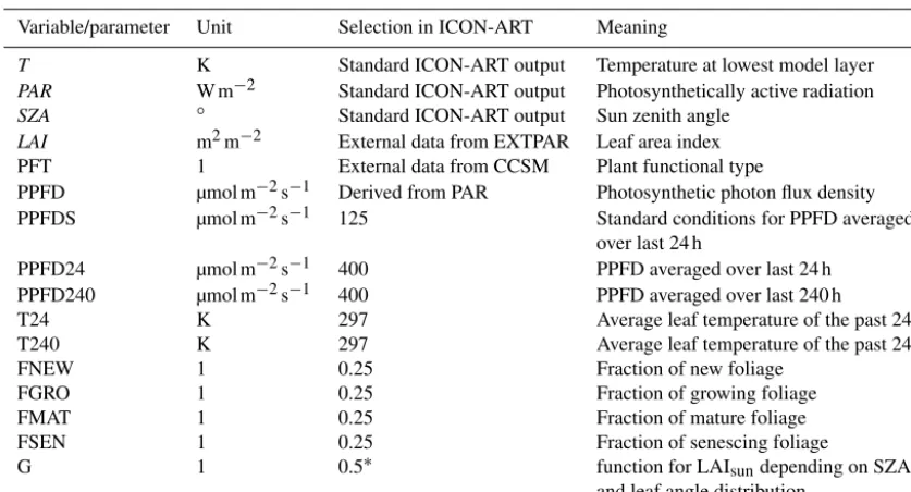
Table 4.Parameters for MEGAN-Online used for this study. Time-dependent parameters are written in italic letters.
Variable/parameter Unit Selection in ICON-ART Meaning
T K Standard ICON-ART output Temperature at lowest model layer
PAR W m−2 Standard ICON-ART output Photosynthetically active radiation
SZA ◦ Standard ICON-ART output Sun zenith angle
LAI m2m−2 External data from EXTPAR Leaf area index PFT 1 External data from CCSM Plant functional type
PPFD µmol m−2s−1 Derived from PAR Photosynthetic photon flux density PPFDS µmol m−2s−1 125 Standard conditions for PPFD averaged
over last 24 h
PPFD24 µmol m−2s−1 400 PPFD averaged over last 24 h PPFD240 µmol m−2s−1 400 PPFD averaged over last 240 h
T24 K 297 Average leaf temperature of the past 24 h T240 K 297 Average leaf temperature of the past 240 h
FNEW 1 0.25 Fraction of new foliage
FGRO 1 0.25 Fraction of growing foliage
FMAT 1 0.25 Fraction of mature foliage
FSEN 1 0.25 Fraction of senescing foliage
G 1 0.5∗ function for LAIsundepending on SZA
and leaf angle distribution
∗Value given by Dai et al. (2004).
ICON-ART and therefore have to be estimated (spatiotempo-rally constant). This could be a further source of uncertainty among the overestimation of the LAI. A sensitivity study by varying 24 and 240 h averages of PAR and leaf temperature results in changes of the emissions up to 13 % in the max-imum for the ranges of 0 to 800 µmol m−2s−1 of PAR and within the temperature range of 283 to 296 K (not shown).
For standard conditions, we use the average photosyn-thetic photon flux density (PPFDS) of the values given by Guenther et al. (2012): PPFDS=125 µmol m−2s−1. Table 4 summarises the input of MEGAN-Online and the parameter selection as used for this study.
In the following we compare the results from three emis-sion scenarios: MEGAN-MACC, MEGAN-Online LAI and MEGAN-Online LAIsun. MEGAN-MACC uses the
emis-sions from the external data set. The MEGAN-Online sce-narios use the online calculated emissions by using LAI (MEGAN-Online LAI) and the LAI that is lit by sun (MEGAN-Online LAIsun).
Figure 7 shows the results of the three emission scenarios based on simulations using the numerical weather prediction physics package. The biogenic emission inventory MEGAN-MACC consists of monthly mean values of the MEGAN2.1 model (see Sect. 3.1.4). Therefore, the diurnal cycle is ne-glected in the inventory. The time series in Fig. 7 are spa-tially averaged over South America, where the global max-imum of biogenic emissions occurs; see Fig. 6. The inven-tory MEGAN-MACC, represented by the red dashed line in Fig. 7, is linearly interpolated between June and July. How-ever, as acetone is emitted as by-product of photosynthesis
Figure 7.Acetone emission comparison of MEGAN-MACC (red dashed), MEGAN-Online LAI (blue) and MEGAN-Online LAIsun (orange) averaged over South America (77 to 44◦W and 27◦S to 2◦N) in June 2004.
(Jacob et al., 2002), the diurnal cycle in the emission should be considered.
With online emissions, it is now possible to capture the diurnal cycle in the emissions of acetone. The acetone online emissions are non-zero during the night which is consistent with the literature (e.g. Shao and Wildt, 2002).
The emissions of the MEGAN-Online LAI scenario are more than twice higher than that of MEGAN-MACC. In con-trast to this, the emissions due to LAIsunof Eq. (7) have the
Table 5.Global acetone emission fluxF(Tg yr−1) for the scenarios of Fig. 7 calculated for the year 2004. Prescribed anthropogenic and biomass burning emissions are included and account for 1.2 and 2.2 Tg yr−1, respectively.
Scenario F
(Tg yr−1)
MEGAN-MACC 41
MEGAN-Online LAI 92 MEGAN-Online LAIsun 42
comparable with the emission fluxes mentioned, for exam-ple, in Jacob et al. (2002), Fischer et al. (2012), Guenther et al. (2012) and Khan et al. (2015). This means that the parametrisation according to Eq. (7) can be used for investi-gation of the effect of the diurnal cycle on the emissions and the acetone VMR in the atmosphere for future simulations.
In order to investigate the influence of the parametrisation of LAI by Eq. (7) we show in Fig. 8 the distributions of LAI and LAIsun, together with its influence on the acetone
emis-sion. As expected, large values in LAI (top panel) occur over the Amazon region in South America as well as in central Africa, where the acetone VMR in Fig. 6 also maximises. In addition, the forest areas in the east of Canada, northern Europe and Siberia show large values of the LAI. In these regions, the LAI is in the order of 3 to 6 m2m−2.
For the used solar zenith angle of 10.3◦, the parametrisa-tion according to Eq. (7) smoothes and reduces the LAI to values around 1 m2m−2(Fig. 8b). But for the less vegetated regions such as deserts (Sahara or Atacama), the distribution of LAIsunshows nearly no response to the parametrisation of
Dai et al. (2004).
In the MEGAN model the emission mass flux density is proportional to LAI (Guenther et al., 2012). That is why the resulting emissions in MEGAN-Online depend linearly on the LAI for each shown plant type (Fig. 8c). The highest sen-sitivity on LAI can be seen for broadleaf trees in the tropics. Thus, the parametrisation of the LAI according to Dai et al. (2004) can lead to a reduction of the emissions of the order of a factor of 2 to 3 in these regions.
To conclude, the correct treatment of LAI is crucial to get realistic results of the emissions in MEGAN. The parametri-sation according to Dai et al. (2004) leads to emission flux densities of the same order of magnitude as in the offline data set MEGAN-MACC (see Fig. 7). Further investigation of this will be presented in Sect. 7.
4 Parametrisation of tracer depletion with simplified OH chemistry
The main atmospheric sink for VOCs is the reaction with OH. Here, we illustrate the new OH depletion mechanism as implemented in ICON-ART. This parametrisation calculates
Figure 8.Distribution of(a)LAI in ICON and(b)LAIsun accord-ing to Eq. (7) for a solar zenith angle of 10.3◦, together with(c) de-pendence of the acetone emission mass flux density on the LAI for different vegetation types in MEGAN-Online withT =300 K and PPFD=400 µmol m−2s−1.
the loss rate of the tracers dependent on space and time and can replace the globally constant lifetime as mentioned in Rieger et al. (2015). As an example, we illustrate the mecha-nism with acetone as one member of the VOCs.
4.1 Troposphere and UTLS region
As the tracer depletion mechanism by reaction with OH, de-scribed below, includes photolysis of ozone we first explain how photolysis rates are treated in ICON-ART.
used is based on the climatology of Global and regional Earth-system (Atmosphere) Monitoring using Satellite and in situ data (GEMS; Hollingsworth et al., 2008).
The photolysis module covers roughly the wavelength re-gion from 170 up to 850 nm, binned into 18 wavelength bins. Thus, it is possible to accurately calculate photolysis rates from the troposphere up to the stratosphere. For the simula-tions within this study the average cloud mode of Cloud-J is used.
The tropospheric OH concentration is calculated accord-ing to a simplified model, shown, for example, by Jacob (1999); see Reactions (R1) to (R8). In this model, ozone is photolysed producing an oxygen atom in excited state, O(1D). O(1D)either is quenched by collision with nitrogen (N2) or oxygen (O2) or reacts with H2O, leading to two OH
radicals: O3+hν
JO3
−→ O(1D)+O2, (R1)
N2+O(1D)
kN2
−→ O(3P)+N2, (R2)
O2+O(1D)
kO2
−→ O(3P)+O2, (R3)
H2O+O(1D)
kH2O
−→ 2OH. (R4)
OH is depleted by reaction with either CH4 or CO, the
main sinks for OH (Jacob, 1999): OH+CH4
kCH4
−→ H2O+CH3, (R5)
−→ · · · −→CO+HO2, (R6)
OH+CO M−→,kCO,1 H+CO2, (R7)
OH+CO M−→,kCO,2 HOCO. (R8)
Reaction rates and photolysis rates in this study are de-noted as k and J, respectively. In the following, squared brackets stand for number concentration of the species (molecules per volume unit). According to the reaction sys-tem above, the steady state OH concentration is calculated by the following equation (see Jacob, 1999; Dunlea and Ravis-hankara, 2004; Elshorbany et al., 2016):
[OH] = 2[O(
1D)]k
H2O[H2O]
kCH4[CH4] +(kCO,1+kCO,2)[CO]
, (8)
where[O(1D)]is calculated by assuming a steady state with Reactions (R1) to (R4) resulting in the following formula:
[O(1D)] = JO3[O3]
kO2[O2] +kN2[N2] +kH2O[H2O]
. (9)
In Eqs. (8) and (9), the O3photolysis rateJO3is calculated
by the online photolysis module in ICON-ART (see above in this section). Ozone is provided by the GEMS climatology (Hollingsworth et al., 2008). [H2O]is calculated as part of
the ICON micro-physics (see Sect. 2.1). O2and N2VMRs
are set to 20.946 and 78.084 %, respectively (Brasseur and Solomon, 1995), and converted to number concentrations. The reaction rates in Eqs. (8) and (9) are taken from Sander et al. (2011).
With Eq. (8), the loss rates of CO, CH4and C3H8are
cal-culated as follows:
Li=ki[OH], i∈ {CO,CH4,C3H8}. (10)
Reaction (R5) results in a cascade of fast reactions and finally in a production of CO and is the largest source for at-mospheric CO (Jacob, 1999; Boucher et al., 2001; Seinfeld and Pandis, 2012, pp. 46–47). Since Reaction (R5) is the re-action with lowest rere-action rate of this cascade the chemical production of CO can be estimated as follows:
PCO=kCH4[OH] [CH4]. (11)
As an example, we will focus on acetone in the following. Acetone is depleted either by reaction with OH or by photol-ysis where two channels have to be considered:
CH3C(O)CH3+OH
kacetone
−→ Products, (R9)
CH3C(O)CH3+hν
Jacetone,1
−→ CH3CO+CH3, (R10)
CH3C(O)CH3+hν
Jacetone,2
−→ 2CH3+CO. (R11)
Reaction (R9) has different channels and is abbreviated here. For the reaction ratekacetone, we use the recommended formula of Sander et al. (2011).
Following Reactions (R9) to (R11), the loss rate of acetone is determined by
Lacetone=kacetone[OH] +Jacetone,1+Jacetone,2. (12) We use the mass-weighted mean shown by SPARC (2013) to calculate the lifetime of acetone:
τacetone= R
[CH3C(O)CH3]dV R
Lacetone[CH3C(O)CH3]dV
. (13)
Additionally, the chemical production of acetone due to reaction of propane (C3H8) with OH is considered:
Pacetone=0.736[C3H8] [OH]kC3H8, (14)
wherekC3H8 is the reaction rate of C3H8+OH. The value
0.736 is a result of the two channels of this reaction and is taken from Atkinson et al. (2006).
Besides emissions, Eq. (14) is another important source for atmospheric acetone (e.g. Jacob et al., 2002). The acetone production due to other VOCs is neglected.
4.2 Above the UTLS region
In the stratosphere, the lower VMRs of CO and CH4 in
Eq. (8) lead to increases of OH up to 108molec cm−3in the
highest model layer (about 2 Pa). According to Brasseur and Solomon (1995), however, the OH number concentration at this altitude is of the order of 106molec cm−3. This overesti-mation of the OH concentration in ICON-ART results in too short lifetimes of the tracers and that is why the lifetime of the species is parametrised in another way for stratospheric conditions.
However, the loss rate of acetone with Eq. (12) is also re-alistic above the UTLS region due to the photolytic Reac-tions (R10) and (R11).
Therefore, another mechanism is applied above the UTLS region (indicated by the dashed blue line in Fig. 9) only if no other term is added to the loss rate. The lifetime of CH4is
parametrised pressure-dependent like in the Integrated Fore-cast System (IFS; Simmons et al., 1989). In this parametri-sation, the CH4lifetime in the troposphere is effectively
in-finite and decreases for pressure below 100 hPa; for exam-ple, it is 2000 days at a pressure of 10 hPa. The CO life-time is parametrised in the same way as in the KASIMA model (Karlsruhe SImulation model of the Middle Atmo-sphere) which also depends on pressure, only (Ruhnke et al., 1999; Kouker et al., 1999). The CO lifetime in this parametri-sation at an altitude of 100 hPa is about 1 year and at 10 hPa it is 25 days. The formulae of these two lifetime parametrisa-tions have been published by Stassen (2015). The lifetime of propane is set globally to 14 days (Rosado-Reyes and Fran-cisco, 2007).
In order to be able to investigate processes within the UTLS region, a threshold in CH4 of 1 ppmv (=
10−6mol mol−1) is applied. This value ensures the OH mechanism to be used in the lowermost stratosphere.
In Fig. 9, the zonal maximum of the air pressure where the CH4 VMR decreases below 1 ppmv (blue dashed) is
illustrated along with the zonal minimum of the WMO tropopause pressure (black solid). Additionally, the zonally averaged VMR of CH4 at the tropopause is shown (red
dotted), which ranges from 1.65 (Southern Hemisphere) to 1.7 ppmv (Northern Hemisphere). Due to its relatively long tropospheric lifetime, CH4is well mixed in the troposphere
and the CH4VMR does not decrease below 1 ppmv. Above
the tropopause, the CH4VMR decreases with height because
of higher photolysis rates in the stratosphere.
As can be seen in Fig. 9, the lowest height where the CH4 VMR decreases below 1 ppmv is clearly above the
tropopause so that the OH mechanism is also applied in the lowermost stratosphere.
5 Measurements of acetone
We evaluate our simulations of acetone with observations from (a) the KCMP tall tower measurements in Midwest-ern USA for seasonal and interannual variations, and (b) the
Figure 9. Zonal minimum of tropopause pressure, zonal maxi-mum of 1 ppmv CH4 pressure and zonal mean of CH4VMR at tropopause (rightyaxis) for June 2004 of the OH-chem simulation (see Sect. 6). The 1 ppmv CH4pressure in each column is calculated as the air pressure of the model layer where CH4VMR decreases below 1 ppmv.
IAGOS-CARIBIC airborne measurements in the UTLS re-gion in a similar way as recently published by Jöckel et al. (2016).
A suite of VOCs including acetone at the KCMP tall tower was measured by a proton transfer reaction mass spectrome-ter between July 2009 and August 2012 (Hu et al., 2013). The tower (44.6886◦N, 93.9728◦W; 244 m height above ground) is located at rural area surrounded by croplands. Measure-ments were carried out 185 m above ground level, providing regional representativeness. The overall measurement uncer-tainty for acetone averages about 10 %.
In the ongoing project Civil Aircraft for the Regular Inves-tigation of the atmosphere Based on an Instrument Container (IAGOS-CARIBIC) a fully automated laboratory has been integrated into a modified cargo container (Brenninkmeijer et al., 2007). Measuring about 100 trace gases and aerosol parameters, the IAGOS-CARIBIC laboratory is regularly placed on-board a Lufthansa Airbus 340-600 passenger air-craft for up to six consecutive flights per month. The cruising altitude of the aircraft coincides with the UTLS region where measurements have been rare previously. Between 2005 and 2014, the flights took off from Frankfurt, whereas the flights nowadays start at Munich in Germany to many interconti-nental destinations. We use the acetone measurements from IAGOS-CARIBIC to compare them with the different inno-vations in ICON-ART (see Sect. 7.3). For our calculations, we use the data of the IAGOS-CARIBIC flights with the numbers 110 to 261 and 373 to 528. Statistics of the desti-nations of these flights can be found in Appendix B.
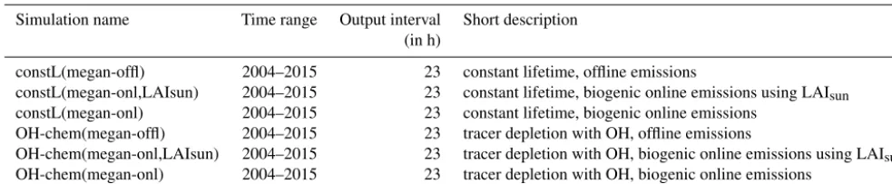
6 Description of the ICON-ART simulations
OH-Table 6.Technical description of the simulations used in this study. For the emission inventories used see Table 3. Horizontal resolution for the simulations is R2B04 with an advective model time step of 460 s. Output is given on model layers.
Simulation name Time range Output interval Short description (in h)
constL(megan-offl) 2004–2015 23 constant lifetime, offline emissions
constL(megan-onl,LAIsun) 2004–2015 23 constant lifetime, biogenic online emissions using LAIsun constL(megan-onl) 2004–2015 23 constant lifetime, biogenic online emissions
OH-chem(megan-offl) 2004–2015 23 tracer depletion with OH, offline emissions
OH-chem(megan-onl,LAIsun) 2004–2015 23 tracer depletion with OH, biogenic online emissions using LAIsun OH-chem(megan-onl) 2004–2015 23 tracer depletion with OH, biogenic online emissions
chem(megan-onl) hereafter. They are summarised in Table 6 from a technical point of view.
The simulations are performed with a horizontal resolu-tion of R2B04 (characteristic length of about 160 km). For output, they are interpolated to a regular 1◦×1◦ longitude-latitude grid. The lowest 46 of total 90 vertical layers are illustrated in Fig. 1. The advective model time step is set to 460 s. All the simulations include an output interval of 23 h. With this interval, we are able to see the impact of OH on acetone at different times of day without using too many re-sources. Emissions as described in Table 3 are added to the tracers’ VMR in the lowest model layer; see Sect. 3.1.3 for a discussion of this choice.
The meteorological variables such as temperature, pres-sure and three-dimensional wind as well as sea surface tem-perature and sea ice cover are initialised with ERA-Interim on 1 January 2004 at 00:00 UTC in order to cover the IAGOS-CARIBIC time range (2005–2015) with a spin-up period of one year for the chemical tracers. CO and CH4are
initialised based on mean values provided by MACC reanal-ysis of January 2004 (Inness et al., 2013). C3H8is initialised
based on Pozzer et al. (2010). The initial volume mixing ratio of acetone is set globally to 1 pptv. After initialisation ICON-ART runs freely.
constL(megan-offl): the simulation using constant lifetime is the reference simulation for the other simulations. In this simulation, acetone lifetime is set globally to 28 days. This is the mean value of the chemical lifetimes of Jacob et al. (2002), Arnold et al. (2005), Fischer et al. (2012) and Khan et al. (2015). The lifetime of C3H8is set to 14 days. That of
CO and CH4 are parametrised as described in Sect. 4.2 for
the whole atmosphere.
constL(megan-onl,LAIsun): simulation of online biogenic emissions of acetone is performed in this simulation where the offline biogenic acetone emissions in constL(megan-offl) are replaced by MEGAN-Online LAIsun(see Sect. 3.2).
constL(megan-onl): simulation of online biogenic emis-sions of acetone is performed in this simulation where the offline biogenic acetone emissions in constL(megan-offl) are replaced by MEGAN-Online LAI.
OH-chem(megan-offl): in the simulation including the sim-plified OH chemistry, the mechanism as illustrated in Sect. 4 is used for depletion of the tracers and therefore replaces the constant lifetime of constL(megan-offl).
OH-chem(megan-onl,LAIsun): in this simulation, the of-fline biogenic acetone emissions in OH-chem(megan-offl) are replaced by MEGAN-Online LAIsun.
OH-chem(megan-onl): here, the biogenic emissions of acetone are replaced by MEGAN-Online LAI.
7 Results
7.1 Comparison of the ICON-ART simulations to ground-based measurements
Near-surface measurements of acetone are rare and no stan-dard output of operational measurements. There are data available for several measurement campaigns such as by Schade and Goldstein (2006) or Fares et al. (2012) but only within 1 year. As our focus in this study is on the interan-nual variation of acetone in a climatological sense we here compare our simulations with the tall tower measurements in Minnesota, USA, performed by Hu et al. (2013).
Acetone was measured at a height of 185 m above ground so that the measurements should not be affected too much by local effects such as specific plants at the site. The mea-surements cover a 2-year period from 2010 to 2011 and have already been used for a comparison to a global model (Hu et al., 2013).
In Fig. 10, we show the results of the three OH-chem sim-ulations together with the full observational time series. For the simulated time series, the horizontal grid point closest to the observation site is chosen and linearly vertically inter-polated in geometric height to the measurement height. We cannot expect to simulate the full variability of the time series due to the coarse resolution of the simulation.
Figure 10. Measured (black) and simulated (red: offl); blue: onl); orange: OH-chem(megan-onl,LAIsun)) acetone VMR interpolated to the observation site in Minnesota (USA); see Hu et al. (2013). The measurement error of 10 % is not included in the figure.
In contrast to this, the simulated acetone VMR of OH-chem(megan-offl) and OH-chem(megan-onl,LAIsun) during the summer months (June to August) slightly underestimate the measurements. Altogether, these two time series resem-ble each other and are in good agreement with the observa-tions. This confirms the previous results related to Figs. 7 and 8, where we have already discussed that the parametrisation of the LAI according to Eq. (7) leads to results comparable with the inventory MEGAN-MACC.
Altogether, we conclude that the emission module per-forms well in comparison to the ground-based measure-ments. The average annual cycle is reflected in all our simu-lations. The overestimated OH-chem(megan-onl) simulation can be explained by a too large leaf area index (see Fig. 8). Especially the offl) and OH-chem(megan-onl,LAIsun) simulations coincide well with the observed time series.
7.2 Profile of the acetone lifetime in the OH-chem simulations
In Fig. 11, profiles of the annual mean acetone global life-time according to Eq. (13) during the OH-chem(megan-offl) simulation are shown. For pressures higher than 900 hPa, the photolysis rates in Eq. (12) get lower which means that the lifetime is dominated by the depletion with OH, only, lead-ing to lifetimes up to 70 days. In the troposphere and UTLS region, both mechanisms seem to have significant influence on the acetone lifetime. Due to the decrease in water vapour above the tropopause the production of OH by Reaction (R4) decreases. Additionally, the photolysis rates increase in the stratosphere for pressures below 50 hPa so that the influence of the OH depletion is negligible and the acetone lifetime decreases below 1 day.
When calculating the global annual mean tropospheric lifetime of acetone according to Eq. (13) in the OH-chem simulations, we derive a value (33 days) comparable to the
Figure 11.Global lifetime of acetone according to Eq. (13) in the OH-chem simulations averaged for each year. Definition of global lifetime by SPARC (2013) evaluated at each model layer.
one (35 days) by Arnold et al. (2005) who also used the def-inition of SPARC to calculate the acetone lifetime.
7.3 Comparison of the ICON-ART simulations with airborne measurements
Figure 12. Annual cycles of the acetone VMR of(a)IAGOS-CARIBIC measurements and due to offline MEGAN-MACC(b, e) and MEGAN-Online biogenic emissions with LAIsun(c, f)and LAI(d, g). Acetone VMR is shown±3 km around the WMO tropopause for constL (first row) and OH-chem simulations (second row). Data are limited to the mid-latitudes between 35 to 75◦N and to the pressure range between 180 and 280 hPa. The acetone VMR in the IAGOS-CARIBIC measurements increases up to 1700 pptv in the maximum.
In the panels of Fig. 12, the simulated acetone VMR is linearly interpolated in pressure, longitude, latitude and time to the IAGOS-CARIBIC flights (see Eckstein et al., 2017). For calculation of the tropopause height we use the data sets which are most convenient for the measurements and simulations: the underlying temperature profiles for tropopause height in the IAGOS-CARIBIC measurements are derived from ERA-Interim profiles, whereas the sim-ulated tropopause height is calcsim-ulated directly during run-time of ICON-ART (see Sect. 2.1). We limit the IAGOS-CARIBIC flights (and correspondingly the model data) to latitudes between 35 and 75◦N and exclude descents and as-cents of the aeroplane by using data inside the pressure range of 280 and 180 hPa (similar to Jöckel et al., 2016).
Figure 12 demonstrates that the general annual cycle of acetone can be reproduced with ICON-ART. Maximum val-ues in the acetone VMR of all ICON-ART simulations occur between June and August, when the measurements also max-imise. However, differences in the magnitude can be seen: for the simulations driven by offline emissions (left column) the maximum acetone VMR is underestimated by a factor of 3 with respect to the measurements.
As could be expected from Fig. 7, the annual cycles of ace-tone of constL(megan-onl,LAIsun) and OH-chem(megan-onl,LAIsun) are nearly identical with the respective offline emissions simulations except for slightly higher values in case of the LAIsun simulations. Thus, by parametrising the LAI according to Dai et al. (2004) the online biogenic emis-sions in ICON-ART are in good agreement with the offline data set MEGAN-MACC.
In contrast to this, MEGAN-MACC does not include a parametrised LAI – at least, there is no information given about it in Sindelarova et al. (2014). This is why the result-ing acetone VMR of the more than twice larger online emis-sions using LAI have been suggested to be in agreement with MEGAN-MACC.
The acetone VMR around the tropopause using MEGAN-Online LAI is shown in the rightmost column of Fig. 12. As these emissions are more than twice larger than the offline emissions the acetone VMR is increased in the UTLS region correspondingly. Thus, the differences with reference to ob-servations are reduced but the highest values in the measure-ments can still not be reached (around 1100 pptv compared to 1700 pptv in the measurements). Apart from the values in the maximum, Fig. 12d using MEGAN-Online LAI com-bined with constant lifetime of acetone shows the best agree-ment with the observations in the upper troposphere: the ace-tone VMR during winter and “near-summer” only differs by 100 pptv or below.
As already mentioned, the global lifetime of acetone in the OH-chem simulations with a value of 33 days is of the same order of magnitude as in the constL simulations. That is why the maximum values in the acetone VMR in the OH-chem simulations are comparable to the corresponding constL sim-ulations. However, differences occur during winter, when the clearly higher acetone lifetime of about 1.5 years in the OH-chem simulations increases the acetone VMR in the UTLS region. This value is a mid-latitudinal (35 to 75◦N) average for the months December to February in 2005 to 2015 in con-trast to the global annual average mentioned above.
The comparison of Fig. 12f with the observations demon-strates that the acetone VMR is overestimated by a factor of about 1.5 in the winter months December to February in the upper troposphere. In the lowermost stratosphere and espe-cially above 2 km of the tropopause height, though, the ace-tone VMR is improved using the OH chemistry, where the observations show higher VMRs than for the case of a con-stant lifetime (Fig. 12c).
7.4 Discussion
The findings in the UTLS region seem to be in conflict to the near-surface comparison of Fig. 10. In Fig. 12 the megan-onl simulations fit best to the measurements, whereas the megan-offl and megan-onl,LAIsun simulations agree well with the ground-based observations. Several reasons could explain this discrepancy which will be discussed below:
1. uncertainty in the sources of acetone; 2. uncertainty in the depletion of acetone; 3. uncertainty in the model transport; 4. uncertainty in the tropopause height. 7.4.1 Uncertainty in the sources of acetone
As mentioned above acetone is directly emitted and is chem-ically produced by oxidation of monoterpenes, propane and isoalkanes (e.g. Jacob et al., 2002).
Emissiondata sets generally are highly uncertain. Sinde-larova et al. (2014) estimated an uncertainty in MEGAN-MACC for isoprene emissions of globally 14 %. For other VOCs, it could be even higher (e.g. 48.5 % by Williams et al., 2013). Oda et al. (2015) introduced a new method to calcu-late the emission uncertainty in a spatially dependent manner which resulted in a local uncertainty up to 200 % for CO2.
Based on Williams et al. (2013), we here assume the uncer-tainty in the acetone emissions to be of the order of 50 % which leads to a total uncertainty of 20 Tg yr−1.
Acetone production due to oxidation of propane: in the emission inventories used for propane (see Table 3) anthro-pogenic, biogenic and biomass burning emissions amount to 4.0, 0.03 and 1.7 Tg(propane)yr−1. The corresponding acetone production using the acetone yield of 0.736 (see
Eq. 14) is about 5 Tg(acetone)yr−1. These values are close to that in the literature (Singh et al., 1994; Khan et al., 2015) although Singh et al. (1994) assume the global source of propane to be significantly higher, of the order of 15 to 20 Tg(propane)yr−1. A propane source of the order of 15 Tg(propane)yr−1 is also used in GEOS-Chem (Jacob et al., 2002; Fischer et al., 2012; Brewer et al., 2017). Due to the difference of about 10 Tg(propane or acetone)yr−1in our configuration compared to that in GEOS-Chem we as-sume an uncertainty of this order for the acetone production in ICON-ART.
Acetone production due to isoalkanes: according to Jacob et al. (2002), it is of the order of 6 Tg yr−1.
Acetone production due to monoterpenes: we perform a test simulation using the monoterpenes in MEGAN-Online and calculate an acetone production of 8 Tg yr−1 using the same method as Brewer et al. (2017). They used a molar ace-tone yield by oxidation of monoterpenes of 0.116. However, the explicit treatment of monoterpene chemistry could lead to a much higher acetone production, e.g. 46 Tg yr−1by Khan et al. (2015).
Table 7 summarises our uncertainty estimates. The sum of all uncertainties is of the order of the acetone source itself which could explain the underestimation of acetone in the UTLS region.
The comparison to ground-based measurements at a site in Minnesota in Fig. 10 suggests that the emissions are well known in this specific region but the uncertainty could be higher in other parts of the world such as the tropical rain-forests.
7.4.2 Uncertainty in depletion of acetone
Acetone is depleted by photolysis and reaction with OH; see Reactions (R9) to (R11). The functions used for reaction rates from Sander et al. (2011) include uncertainties. Due to their non-linear dependence on temperature small variations in the reaction rates can have great effect on the depletion of acetone.
In addition, for OH no VOC sink is included in our sim-plified approach. Especially isoprene is responsible for up to 70 % of the OH sink as measured by Hansen et al. (2014) and Rickly et al. (2017) close to the isoprene source in a forest.
Typical values of the OH reactivity during daytime mea-sured by Hansen et al. (2014) in a boreal forest in northern Michigan (USA) are around 20 s−1. In our model, the OH re-activity over North America is around 5 s−1, so a factor of 4
lower than measured in this region.
Table 7.Estimated uncertainty of acetone emissions and precursor species in Tg(acetone)yr−1.
Quantity Accounted for Uncertainty in ICON-ART2.0 (Tg yr−1)
Direct emissions X 20
Oxidation of propane X 10
Oxidation of isoalkanes – 6
Oxidation of monoterpenes – 8
7.4.3 Uncertainty due to model transport
We performed a test simulation using another physics pack-age in ICON. Especially, this physics packpack-age includes other treatment of convection and vertical diffusion. Differences to the simulations in Fig. 12 were clearly visible in the UTLS region including a shifted annual cycle similar as in the chemistry climate model EMAC (Jöckel et al., 2016). Fur-ther investigation of this issue is needed.
This example demonstrates that the model transport in at-mospheric models also includes uncertainties which how-ever are hard to quantify. With the resolution of R2B04 (∼160 km) used in this study, boundary layer convective pro-cesses could be underestimated leading to a too slow trans-port into the free troposphere.
7.4.4 Uncertainty in the tropopause height
For investigation of acetone in the UTLS region we use the WMO thermal tropopause height, derived from ERA-Interim or ICON-ART temperature. To investigate the uncertainty in the tropopause height another definition could be used for future simulations and especially for the measurements such as the definition derived from ozone as described by Sprung and Zahn (2010) or the dynamical tropopause height.
Higher or lower tropopause height in the measurements as well as in the model simulations could influence the clima-tologies in Fig. 12 since the acetone VMR depends on height, especially in the UTLS region.
7.4.5 Summary of the uncertainties
As could be shown in the previous sections the uncertain-ties in our simulations due to simplifications are quite large. These uncertainties can explain the mentioned conflict be-tween Figs. 10 and 12.
To reduce the uncertainties further investigation is needed – the correct treatment and reduction of emission uncertain-ties in the inventories is current subject of research (e.g. Oda et al., 2015). The inclusion of monoterpenes and isoalkanes could improve the acetone source in our simulations. The in-clusion of isoprene could lead to an improvement of OH in the source regions of acetone (Hansen et al., 2014). For eval-uation of the model transport vertical profiles either from
air-craft measurements or from satellites should be used in the future if available. In addition, the model transport near the surface could be investigated by introduction of a very short-lived substance.
8 Conclusions and outlook
We introduce the recently developed module for including emissions from external data sources in ICON-ART. The module reads the data interpolated to the ICON grid, inter-polating to the simulation time and adding to the trace gas volume mixing ratio in ICON-ART. For this, the number of lowest model layers of the emissionsnlev,emihas to be
speci-fied where we show a sensitivity test by varying this number. Differences only occur in the height of the emissions itself.
Therefore, the tracer mixing ratio above the emission heightnlev,emiis independent of the choice ofnlev,emi. Since
the aim of this study is the simulation of acetone in the upper troposphere and lowermost stratosphere (UTLS), we select
nlev,emi=1.
In addition, we demonstrate the online biogenic emission model MEGAN2.1 in the configuration as implemented in ICON-ART including two parametrisations of the leaf area index (LAI): the unparametrised LAI of ICON (MEGAN-Online LAI scenario) and the LAI parametrised according to Dai et al. (2004) (MEGAN-Online LAIsun).
Emissions using in MEGAN-Online LAI are twice larger than emissions of the offline emission inventory MEGAN-MACC. The emissions of MEGAN-Online LAIsunare
com-parable to MEGAN-MACC in terms of global means and can therefore be used for investigating the influence of the diur-nal cycle on acetone in the atmosphere.
Furthermore, we present a simplified parametrisation to deplete chemical species by reaction with OH. The OH con-centration is calculated as steady state: it is produced by pho-tolysis of ozone and reaction of the produced O(1D) with water vapour. It is depleted by reactions with CH4and CO.
With these new features, it is now possible to simulate volatile compounds (VOCs) with ICON-ART reliably. We il-lustrate this with acetone as one member of the VOCs.
Compared to ground-based measurements of Hu et al. (2013), our simulations generally show a comparable sea-sonal cycle. Due to the higher emissions the acetone volume mixing ratio is overestimated with MEGAN-Online LAI. In contrast to this, the simulations with offline emissions and online biogenic emissions of MEGAN-Online LAIsunare in
good agreement with the observations with slight underes-timation during summer. This demonstrates that the correct treatment of the LAI in MEGAN2.1 is crucial to get realistic results for online biogenic emissions. Further investigation of the representation of the emissions in MEGAN2.1 will fol-low in the future.
IAGOS-CARIBIC project in the UTLS region. With offline emis-sions and with online emisemis-sions of MEGAN-Online LAIsun
the acetone VMR in the UTLS region is underestimated by a factor of 3. Correspondingly, it is increased by using the unparametrised LAI of ICON for online emissions. The sim-plified OH chemistry leads to a higher acetone lifetime espe-cially during winter which results in an overestimation of the acetone VMR within December and February by a factor of about 1.5. On the other hand, the acetone VMR in the low-ermost stratosphere is improved by using the OH depletion mechanism.
Altogether, we show that the general acetone annual cycle is well represented in the model compared to the ground-based observations as well as to airborne IAGOS-CARIBIC measurements with a maximum during summer and a mini-mum during winter. Considering the acetone distribution in the lowest model layer we demonstrate that the presented emission module performs well. In addition, the calculated tropospheric acetone lifetime of 33 days is in good agree-ment with Arnold et al. (2005) who used the same method to derive it. This value suggests that the new parametrisation of tracer depletion with OH is a good estimate of the OH concentration in the troposphere.
We also estimate the uncertainties in our simulations and further investigation should include the following aspects: adding further sources of acetone such as oxidation of higher VOCs, inclusion of isoprene as sink of OH, evaluation of the model transport by comparison to vertical profile mea-surements and using different definitions of the tropopause height.
Code availability. Currently the legal departments of the Max Planck Institute for Meteorology (MPI-M) and the DWD are fi-nalising the ICON licence. If you want to obtain ICON-ART you will first need to sign an institutional ICON licence, which you will get by sending a request to [email protected]. In a second step you will get the ART licence by contacting Bernhard Vogel ([email protected]).
Appendix A: Predictor–corrector method
In this section, we explain the discretisation method for tracer concentration changes. We here refer to “concentration” as an abbreviation of number concentration (unit molecules per volume unit). Concentrations of tracers are determined by solving the following differential equation:
∂ci(x, t )
∂t =Pi(x, t )−ci(x, t ) Li(x, t ), (A1)
withci,PiandLi as concentration, chemical production and loss rate of traceri. Concentration, chemical production and loss rate depend on locationxand timet. In ICON-ART ver-sion 1.0, this equation was discretised with the explicit Euler method (Rieger et al., 2015), omitting the index i and the location dependence:
c(t+e)1t =c(te)+
Pt−c(te)Lt
1t. (A2)
Too low values of the tracer’s lifetime can lead to solu-tions that do not converge to the differential Eq. (A1). Since fully implicit methods generally are expensive in computa-tion resources, Seinfeld and Pandis (2012, pp. 1125–1126) suggest a two-step predictor–corrector discretisation method for solving Eq. (A1) which is discussed in this section. This method reasonably closes the gap between the low compu-tation effort for explicit discretisation methods on the one hand and the accuracy and stability of implicit methods on the other hand.
Please note that the lifetime τt in this section is the re-ciprocal value of the loss rate: τt=1/Lt (in contrast to the definition of SPARC used in the other sections).
Generally, Eq. (A1) can be discretised implicitly as fol-lows (Seinfeld and Pandis, 2012, pp. 1125–1126):
c(t+ipc1t) =
c(ipc)t (τt+1t+τt−1t )+0.51t (Pt+1t+Pt) (τt+1t+τt) τt+1t+τt+1t
. (A3)
Lifetimes and productions of the next time step, denoted by indext+1t, are not defined at time stept. That is why they have to be approximated before Eq. (A3) can be evalu-ated.
In a first step, called the predictor step, the new concentra-tionsc∗are approximated by assuming constant lifetime and production (τt+1t=τt andPt+1t=Pt):
c∗=
ct(2τt−1t )+21t τtPt 2τt+1t
. (A4)
In this study, these concentrations are calculated for CH4,
CO, propane and acetone. This is an inaccurate estimation of the concentrations of the next time step since lifetime and production both can vary within one time step (Seinfeld and Pandis, 2012, pp. 1125–1126). For improving accuracy, the lifetimes and productions of the next time step are approxi-mated with thec∗of Eq. (A4). For that purpose,c∗is used for calculating a new OH number concentration,[OH]∗, as described in Sect. 4.1. In turn, with[OH]∗, the lifetimes and chemical productions of the next time step can be approxi-mated, denoted asτ∗andP∗, respectively.
Then, the so-called corrector step can be executed in order to get the tracer concentrations of the next time step by re-placingτt+1tandPt+1t in Eq. (A3) by their approximations
τ∗andP∗, respectively:
c(tpc+1t) =c (pc)
t (τ∗+τt−1t )+0.51t (P∗+Pt) (τ∗+τt)
τ∗+τt+1t
. (A5)
If 1t becomes larger than the expression τ∗+τt, this method also can become unstable.
To illustrate this, consider the following example by as-suming the chemical productionP in Eq. (A5) to be zero, i.e.
P∗=Pn=0 and additionallyτ∗+τn−1t <0. In this case, the concentration of the next time stepc(tpc+1t) becomes nega-tive which obviously shows that the numerical solution does not converge the physical solution of the differential equation of Eq. (A1.)
That is why we use the fully implicit Euler method assum-ing constant lifetime and chemical production if the lifetime gets lower than1t:
ct(+i)1t =Ptτt+
ct(i)−Ptτt
exp
−1t
τt
Appendix B: Statistics of the CARIBIC flights used Here, we show the destinations of all the CARIBIC flights used in the results. The statistics can be found in Table B1. For this, we counted return flights as one flight and did not count stopovers of the aircraft as separate flights.
Table B1. Frequency of occurrence of the destinations in the CARIBIC flights used for the climatologies in Sect. 7. The total number of different flights is 113.
Destination Number of flights
Manila (Philippines)a 21
Chennai (India) 18
Caracas (Venezuela) 11 Kuala Lumpur (Malaysia)b 8 São Paulo (Brazil) 8 Vancouver (Canada) 8 Santiago (Chile)c 7 Seoul (South Korea) 7 San Francisco (USA) 7 Los Angeles (USA) 4
Tokyo (Japan) 3
Toronto (Canada) 2
Denver (USA) 2
Houston (USA) 1
Bogota (Columbia) 1 Rio de Janeiro (Brazil) 1
Beijing (China) 1
Cape Town (South Africa) 1 Mexico City (Mexico) 1 Hong Kong (China) 1