Geosci. Model Dev., 6, 1275–1298, 2013 www.geosci-model-dev.net/6/1275/2013/ doi:10.5194/gmd-6-1275-2013
© Author(s) 2013. CC Attribution 3.0 License.
EGU Journal Logos (RGB)
Advances in
Geosciences
Open Access
Natural Hazards
and Earth System
Sciences
Open AccessAnnales
Geophysicae
Open AccessNonlinear Processes
in Geophysics
Open AccessAtmospheric
Chemistry
and Physics
Open AccessAtmospheric
Chemistry
and Physics
Open Access DiscussionsAtmospheric
Measurement
Techniques
Open AccessAtmospheric
Measurement
Techniques
Open Access DiscussionsBiogeosciences
Open Access Open Access
Biogeosciences
Discussions
Climate
of the Past
Open Access Open Access
Climate
of the Past
Discussions
Earth System
Dynamics
Open Access Open Access
Earth System
Dynamics
DiscussionsGeoscientific
Instrumentation
Methods and
Data Systems
Open Access
Geoscientific
Instrumentation
Methods and
Data Systems
Open Access DiscussionsGeoscientific
Model Development
Open Access Open Access
Geoscientific
Model Development
DiscussionsHydrology and
Earth System
Sciences
Open AccessHydrology and
Earth System
Sciences
Open Access DiscussionsOcean Science
Open Access Open Access
Ocean Science
DiscussionsSolid Earth
Open Access Open Access
Solid Earth
Discussions
The Cryosphere
Open Access Open Access
The Cryosphere
DiscussionsNatural Hazards
and Earth System
Sciences
Open Access
Discussions
A cloud chemistry module for the 3-D cloud-resolving mesoscale
model Meso-NH with application to idealized cases
M. Leriche, J.-P. Pinty, C. Mari, and D. Gazen
Laboratoire d’A´erologie, CNRS/INSU, UMR5560, Toulouse, France Correspondence to: M. Leriche ([email protected])
Received: 19 January 2013 – Published in Geosci. Model Dev. Discuss.: 14 February 2013 Revised: 5 July 2013 – Accepted: 8 July 2013 – Published: 22 August 2013
Abstract. A complete chemical module has been developed
for use in the Meso-NH three-dimensional cloud resolv-ing mesoscale model. This module includes gaseous- and aqueous-phase chemical reactions that are analysed by a pre-processor generating the Fortran90 code automatically. The kinetic solver is based on a Rosenbrock algorithm, which is robust and accurate for integrating stiff systems and es-pecially multiphase chemistry. The exchange of chemical species between the gas phase and cloud droplets and rain-drops is computed kinetically by mass transfers considering non-equilibrium between the gas- and the condensed phases. Microphysical transfers of chemical species are considered for the various cloud microphysics schemes available, which are based on one-moment or two-moment schemes. The pH of the droplets and of the raindrops is diagnosed separately as the root of a high order polynomial equation. The chem-ical concentrations in the ice phase are modelled in a single phase encompassing the two categories of precipitating ice particles (snow and graupel) of the microphysical scheme. The only process transferring chemical species in ice is reten-tion during freezing or riming of liquid hydrometeors. Three idealized simulations are reported, which highlight the sen-sitivity of scavenging efficiency to the choice of the micro-physical scheme and the retention coefficient in the ice phase. A two-dimensional warm, shallow convection case is used to compare the impact of the microphysical schemes on the temporal evolution and rates of acid precipitation. Acid wet deposition rates are shown to be overestimated when a one-moment microphysics scheme is used compared to a two-moment scheme. The difference is induced by a better pre-diction of raindrop radius and raindrop number concentra-tion in the latter scheme. A two-dimensional mixed-phase squall line and a three-dimensional mixed-phase supercell
were simulated to test the sensitivity of cloud vertical trans-port to the retention efficiency of gases in the ice phase. The 2-D and 3-D simulations illustrate that the retention in ice of a moderately soluble gas such as formaldehyde substan-tially decreases its concentration in the upper troposphere. In these simulations, retention of highly soluble species in the ice phase significantly increased the wet deposition rates.
1 Introduction
More than 50 % of the Earth’s surface is under cloud and several studies have shown that clouds interact with chemi-cal species in many ways, over a wide range of schemi-cales, from micrometres up to thousands of kilometres. On global and regional scales, clouds have a major impact on the compo-sition of the troposphere through multiphase removal pro-cesses (Tost et al., 2007). The impact of clouds on the ozone budget and on simple soluble compounds, such as hydro-gen peroxide, has been well assessed (Lelieveld and Crutzen, 1991; Monod and Carlier, 1999). However, there are still uncertainties concerning the impact of cloud vertical trans-port of chemical species by deep convection on the upper troposphere (UT) composition, and about the impact of the chemical reactivity of organic compounds in clouds on the formation of secondary organic aerosol (SOA). For instance, the source of HOxin the deep convective tropical cloud
out-flow needs more investigation since the production of ozone in the UT is almost proportional to the HOx mixing
and theoretical calculations pointing out the possible role of volatile organic compounds associated with sulphur dioxide as precursors of aerosol particles (Waddicor et al., 2012). Or-ganic aerosols affect the earth’s radiative budget by their role in both direct and indirect aerosol forcing (Kanakidou et al., 2005). The majority of the organic fraction of aerosols is suspected to be of secondary origin. However, the sources, chemical composition and formation mechanisms of SOA re-main one of the least understood processes relevant to the at-mosphere (Hallquist et al., 2009). In particular, new routes of SOA formation have been found to comprise the condensa-tion precursors having low volatility that are formed in cloud droplets or raindrops and released in the clear atmosphere when cloud or rain drops evaporate (Chen et al., 2007; Lim et al., 2010; Ervens et al., 2011). However, the potential con-tribution of the aqueous phase reactivity is highly uncertain, as is the case for the chemical nature of the aqueous phase products that are the precursors of the SOA (Hallquist et al., 2009; Ervens et al., 2011).
The importance of the vertical transport of chemical species by convection has been underlined by many au-thors (e.g. Dickerson et al., 1987; Prather and Jacob, 1997; Lawrence and Crutzen, 1998; Mari et al., 2000, 2003). In particular, local convection is a major source of HOxin the
UT (Jaegl´e et al., 1998). This production of HOxin the UT
perturbed by deep convection is mainly due to photochem-ical reactions of hydrogen peroxide, methyl hydroperoxide, and formaldehyde, which are transported from the boundary layer to the UT by convection or arise from secondary pro-duction in the UT (Jaegl´e et al., 1997; Cohan et al., 1999). As these species are soluble, they are also impacted by cloud microphysical processes and aqueous phase chemistry (Barth et al., 2007b). Assessing the budgets of HOxor SOA thus
requires a detailed understanding of the coupling between cloud venting, microphysics and aqueous chemistry.
However, the parameterization of convective transport and gas scavenging at the global scale still remains approximate (Tost et al., 2010) due to the huge number of non-linear pro-cesses and the high variability of the solubility and reactiv-ity of the chemical compounds. Meanwhile, at convective-resolved scale, current computational power enables cloud resolving models (CRM) to be run, where interactions be-tween the cloud microphysics and the chemistry and the ad-vective/turbulent transport of chemical species can be rea-sonably well detailed (Flossmann and Wobrock, 1996; Barth et al., 2001; Yin et al., 2002). As a result, there is a great need to study and develop an efficient gaseous and aqueous chem-ical scheme tightly coupled to the microphysics of mixed-phase clouds in order to evaluate the budget of chemical com-pounds after a perturbation caused by convective events.
A CRM is a powerful tool for studying the complex in-teractions between transport, chemistry and cloud micro-physics. Whether they are used for improving the represen-tation of the vertical redistribution of gases and aerosol parti-cles by convective clouds, or to contribute to the assessment
of SOA formation by cloud processes, CRMs have to inte-grate a cloud chemistry module, as well as an aerosol module and detailed cloud microphysics.
In this study, a cloud chemistry module for the three-dimensional meteorological model Meso-NH (Lafore et al., 1998) is developed and tested. Among the three ingredients – transport, microphysics and chemistry – the coupling be-tween microphysics and chemistry is the most original part of the package, in particular for cases of mixed-phase cloud. The new module takes advantage of the resolved and tur-bulent transport schemes and the mixed-phase cloud micro-physical scheme, which have been continuously improved, in the host model. Moreover, an aerosol module is available in Meso-NH (ORILAM, for Organic Inorganic Lognormal Aerosol Model, Tulet et al., 2005, 2006), although its cou-pling with the cloud chemistry module is not presented in the present work.
First, the chemical module is described, including the de-tailed treatment of the temporal integration of the chemical production and destruction terms and of the cloud micro-physics transfer terms. The diagnostic computation of the pH is also detailed. Then, three applications of the model are pre-sented. The first one is a warm, idealized, two-dimensional precipitating case to focus on the sensitivity of aqueous phase chemistry to the cloud microphysics scheme: one-moment versus two-moment. The second case corresponds to an ide-alized, two-dimensional squall line to underline the effect of the ice phase on cloud chemistry via the retention of chem-ical species when riming or freezing occurs. The last case is the simulation of a mixed-phase, three-dimensional super-cell, which has been widely studied within the framework of a model intercomparison exercise (Barth et al., 2007a). Fi-nally, some perspectives concerning the use of the full pack-age for simulating complex three-dimensional cloud situa-tions are discussed, together with possible extensions of the module.
2 Description of the cloud chemistry module
electricity including, lightning flash production (Barthe et al., 2012). The new cloud chemistry module represents chem-istry processes in both warm clouds and mixed-phase clouds. In nested mode, it is possible to activate the cloud chem-istry module in only the inner domain to save computing time while the coupling models (“father” models) treat the gas phase chemistry only.
Continuity equations for a chemical species X (mol per volume of dry air) in the gas phase and in the aqueous phase are of the form
∂Xg ∂t = ∂Xg ∂t dyn
+ ∂Xg
∂t
chem
+ ∂Xg
∂t others (1) ∂Xw ∂t = ∂Xw ∂t dyn
+ ∂Xw
∂t
chem
+ ∂Xw
∂t others . (2)
In Eq. (2), the subscript “w” stands for either cloud droplets or raindrops. In both equations, the term “dyn” refers to dynamical tendencies by advection and turbulence, which applies to all prognostic scalars in the model. The term “others” describes emission, dry deposition and release from the aqueous phase when evaporation, freezing or riming oc-curs. This point is detailed in Sect. 2.5. For the aqueous phase species, the term others represents the cloud microphysical processes, which depend on the cloud microphysics scheme and are detailed in Sect. 2.2 for warm clouds and in Sect. 2.5 for mixed-phase clouds. Finally, the term “chem” includes gas–liquid transfer and chemical reactions and will be ex-plained in the following subsection. To avoid numerical prob-lems, Eq. (2) is solved only when the liquid water content of cloud water or rainwater goes beyond a threshold value fixed by the user. A typical value is 1×10⁻⁸vol vol−1. If the liq-uid water content is below this value, the concentrations of the chemical species in water are set to zero after transfer to the gas phase. For ions, which are not linked to a gas phase species by dissociation equilibria, the concentrations are set to zero and the associated mass is lost. However, this con-cerns very few species with very low concentrations (inter-mediate sulphur species; see below and Table 3).
2.1 Chemical kinetic scheme
The evolution of the chemical concentrations in the gas- and liquid phases, denoted by the term chem above, of a chemical speciesXis given by the generic set of differential equations:
∂Xg ∂t chem
=Pg−DgXg−ktw
LwXg−
Xw
HeffRT (3) ∂Xw ∂t chem
=Pw−DwXw+ktw
LwXg−
Xw
HeffRT
; (4)
Xg andXw are the concentration of X in the gas phase
and the liquid phases, respectively.PgandPw,andDgand
Dware the gaseous and the aqueous production terms in mol
per volume of dry air s−1, and the gaseous and aqueous de-struction terms in s−1, respectively.Lw is the liquid water
volume ratio (volume of the drops per volume of air).Heff
is the effective Henry’s law constant in mol atm−1.T is the temperature in K andR=0.08206 atm M−1K−1is the uni-versal gas constant. The rate constant of transfer between the gas phase and the aqueous phase ktw in s−1 is the inverse
of the characteristic times for gaseous diffusion and for the interfacial mass transport according to Schwartz (1986):
ktw=
a2w
3−Dgas +4aw
3να
!−1
(5)
aw is the cloud droplet or raindrop radius in m, Dgasis the
gaseous diffusion coefficient taken equal to 10−5m2s−1for all species, ν is the mean molecular speed in m s−1 of the soluble species (see Leriche et al., 2000) andαis the accom-modation coefficient of the soluble species. For cloud droplet and raindrop populations,awis taken as the mean radius of
the respective size distributions. If a one-moment scheme is used, the cloud droplet radius is fixed (aw=10 µm) and the
mean raindrop radius is diagnosed. Bothaware computed if
a two-moment scheme is chosen.
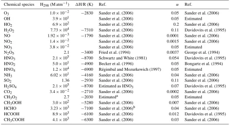
Table 1. Values of Henry’s law constants at 298 K (H298)and associated temperature dependencies (1H/R) and values of mass accommo-dation coefficients (α).
Chemical species H298(M atm−1) 1H/R (K) Ref. α Ref.
O3 1.0×10⁻² −2830 Sander et al. (2006) 0.05 Sander et al. (2006)
OH 3.9×101 Sander et al. (2006) 0.05 Estimated
HO2 6.9×10² Sander et al. (2006) 0.2 Sander et al. (2006)
H2O2 7.73×10⁴ −7310 Sander et al. (2006) 0.11 Davidovits et al. (1995) NO 1.92×10⁻³ −1790 Sander et al. (2006) 0.0001 Sander et al. (2006) NO2 1.4×10⁻² Sander et al. (2006) 0.0015 Sander et al. (2006)
NO3 3.8×10⁻² Sander et al. (2006) 0.05 Estimated
N2O5 2.1 −3400 Fried et al. (1994) 0.0037 George et al. (1994)
HNO3 2.1×10⁵ −8700 Schwartz and White (1981) 0.054 Davidovits et al. (1995)
HNO2 5.0×101 −4900 Becker et al. (1996) 0.05 Bongartz et al. (1994)
HNO4 1.2×10⁴ −6900 R´egimbal and Mozurkewich (1997) 0.05 Estimated
NH3 6.02×101 −4160 Sander et al. (2006) 0.04 Sander et al. (2006)
SO2 1.36 −2930 Sander et al. (2006) 0.11 Sander et al. (2006)
H2SO4 2.1×10⁵ −8700 Estimated as HNO3 0.07 Davidovits et al. (1995)
CO2 3.4×10⁻² −2710 Sander et al. (2006) 0.0002 Sander et al. (2006)
CH3O2 2.7 −2030 Estimateda 0.05 Estimated
CH3OOH 3.0×10² −5280 Sander et al. (2006) 0.007 Sander et al. (2006) HCHO 3.23×10³ −7100 Sander et al. (2006)b 0.04 Sander et al. (2006) HCOOH 8.9×10³ −6100 Sander et al. (2006) 0.012 Davidovits et al. (1995) CH3COOH 4.1×10³ −6300 Sander et al. (2006) 0.03 Sander et al. (2006)
a: estimated from the empirical relation H
ROO2=HROOHHHO2/HH2O2;b: effective value.
Model (TUV, Madronich and Flocke, 1999). The cloud scat-tering is accounted at every time step of the model following Chang et al. (1987). Moreover, the aqueous phase photolysis reactions are modified for increased path length; a factor of 1.6 is used as in Leriche et al. (2000).
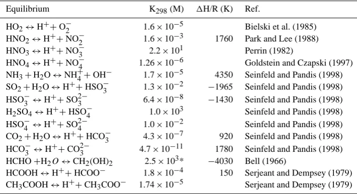
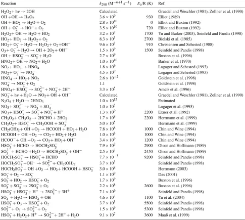
Table 1 lists the chemical species exchanged between the gas- and liquid phases together with the values of their Henry’s law constants and accommodation coefficients. Ta-ble 2 gives the aqueous phase equilibria, which are used to compute the effective Henry’s law constant (except for the HCHO effective Henry’s law value, given in Table 1) and the total species mixing ratio in the aqueous phase. The chemi-cal species involved in equilibria are treated as total species to prevent losing mass within an aqueous phase (see Leriche et al., 2000). This approach allows us to treat the pH as a di-agnosed variable (see Sect. 2.4). Finally, Table 3 presents the aqueous phase chemical mechanism of ReLACS-AQ. This mechanism was developed consistently with the gas phase mechanism ReLACS and based upon two existing reduced aqueous phase mechanisms (Tost et al., 2007; CAPRAM2.4 (Chemical Aqueous Phase RAdical Mechanism) from Er-vens et al., 2003). The resulting reduced ReLACS-AQ mech-anism was tested by comparison with an explicit mecha-nism and with CAPRAM2.4 in the box model M2C2 (Model of Multiphase Cloud Chemistry; Leriche et al., 2003) us-ing the three scenarios from Ervens et al. (2003): urban, ru-ral and marine. Results of the time evolution of chemical
species concentrations showed no significant differences be-tween the full mechanism, the CAPRAM2.4 mechanism and the ReLACS-AQ one (the largest difference was less than 5 %). As the only source of acetic acid in the aqueous phase in ReLACS-AQ is its mass transfer from the gas phase (no source of its precursors in the aqueous phase), which is of mi-nor importance, its aqueous phase reactivity was neglected.
2.2 Cloud microphysics transfer terms
Table 2. Aqueous phase equilibria at 298 K (K298)and associated temperature dependencies (1H/R).
Equilibrium K298(M) 1H/R (K) Ref.
HO2↔H++O−2 1.6×10⁻⁵ Bielski et al. (1985)
HNO2↔H++NO−2 1.6×10⁻³ 1760 Park and Lee (1988)
HNO3↔H++NO−3 2.2×101 Perrin (1982)
HNO4↔H++NO−4 1.26×10⁻⁶ Goldstein and Czapski (1997)
NH3+H2O↔NH+4+OH −
1.7×10⁻⁵ 4350 Seinfeld and Pandis (1998) SO2+H2O↔H++HSO−3 1.3×10⁻² −1965 Seinfeld and Pandis (1998) HSO−3 ↔H++SO2−3 6.4×10⁻⁸ −1430 Seinfeld and Pandis (1998) H2SO4↔H++HSO−4 1.0×10³ Seinfeld and Pandis (1998)
HSO−4 ↔H++SO2−4 1.0×10⁻² Seinfeld and Pandis (1998) CO2+H2O↔H++HCO−3 4.3×10⁻⁷ 920 Seinfeld and Pandis (1998) HCO−3 ↔H++CO2−3 4.7×10⁻¹¹ 1780 Seinfeld and Pandis (1998) HCHO+H2O↔CH2(OH)2 2.5×10³* −4030 Bell (1966)
HCOOH↔H++HCOO− 1.8×10⁻⁴ 150 Serjeant and Dempsey (1979) CH3COOH↔H++CH3COO− 1.74×10⁻⁵ Serjeant and Dempsey (1979)
* K dimensionless
of the microphysical reservoirs. These microphysical transfer terms are computed as follows:
∂Xc
∂t
AUTO
= −∂Xr
∂t
AUTO = −Xc
1
rc
∂rc
∂t
AUTO
(6)
∂Xc
∂t
ACCR
= −∂Xr
∂t
ACCR = −Xc
1
rc
∂rc
∂t
ACCR
(7)
∂Xr
∂t
SEDI
= −Xr
1
rr
∂rr
∂t
SEDI
=Xr
1
rr
∂
∂zFSEDI(rr); (8) rcandrrare the mass mixing ratios of the cloud droplets and
of the raindrops in kg of water per kg of dry air, respectively.
FSEDIis the sedimentation flux of the rain mixing ratio.
The sedimentation flux and the autoconversion and ac-cretion rates depend on the cloud microphysical scheme. In Meso-NH, there are four different ways to calculate these terms. The simplest one computes the cloud microphysics with a one-moment scheme following Kessler (1969) and as-suming a Marshall–Palmer distribution for the raindrops. The second one uses the one-moment scheme for mixed-phase cloud, ICE3 (Pinty and Jabouille, 1998), which is equiva-lent, for the warm part of the scheme, to a Kessler (1969) parameterization assuming a generalized gamma distribution for all hydrometeors including rain. The third one, the C2R2 scheme (Cohard and Pinty, 2000a), is a two-moment scheme for warm cloud, in which the parameterization of the CCN activation follows the diagnostic and integral approach of Twomey (1959), as improved by Cohard et al. (1998). The last one is a two-moment scheme for LES or stratocumulus applications (Khairoudinov and Kogan, 2000). The detailed expressions of each term for the four cloud microphysics
schemes available in Meso-NH can be found in the scientific documentation of Meso-NH (http://mesonh.aero.obs-mip.fr/ mesonh/).
Equations (6), (7) and (8) are integrated into the chemical tendencies (Eqs. 1 and 2) before the kinetic solver is called to resolve the chemical ODE system at each grid point of the computational domain.
2.3 Kinetic solver
The set of non-linear differential equations describing the evolution of chemical species forms a stiff ODE system (Eqs. 3 and 4). Moreover, including an aqueous phase in the chemical scheme increases the stiffness of the numerical ODE (Audiffren et al., 1998), so we substituted the kinetic solvers available in Meso-NH by the Rosenbrock family of solvers described in Sandu et al. (1997).
Rosenbrock solvers are based on multistage implicit meth-ods with an adaptive sub-time step to achieve high order ac-curacy. Each stage of the method needs to solve a system of linear equations by inverting a matrix. This is done with an LU-decomposition method (where L is a lower triangu-lar matrix and U is an upper triangutriangu-lar matrix) and efficient index coding rules that exploit the sparsity of the Jacobian matrix of the chemical system (only the non-zero coefficients are stored).
chemistry, it is useful to order first the gas reactants and then to add the aqueous species.
2.4 pH solver
As the solubility of some important gaseous pollutants de-pends on the pH (by definition pH= −log 10[H+]) of the drops as well as the aqueous phase reactivity, e.g. in sulphate formation, it is crucial to predict the evolution of the pH of the cloud droplets and raindrops. There are two ways to solve the pH in a cloud chemistry module.
The first method explicitly considers all the ionic species by including dissociation equilibria in the aqueous phase chemical mechanism (see Table 2) as backward and forward reactions (e.g. Ervens et al., 2003). Here, the concentration of H+is clearly a prognostic variable. The drawback of this
method is the possibility of numerical instabilities. Because backward and forward reactions of dissociation equilibria are very fast, a very small displacement from equilibrium leads to the sporadic occurrence of abnormally high or low con-centrations of species, which increases the stiffness of the system.
The second method treats the chemical species involved in equilibria as total species; e.g. formic acid in aqueous phase is the sum of the concentration of the dissolved formic acid plus the concentration of formate ions. Using this formula-tion, it is possible to set up an electroneutrality equation of the system and then to simplify it by keeping only the main acids and bases. The complex electroneutrality equation was further developed into a high-order polynomial equation for which the concentration of H+was the physical root to be
se-lected. This operation was carefully conducted using formal calculus software to avoid errors of manipulation. The sim-plified form of the electroneutrality equation deduced from the ReLACS-AQ mechanism is
H++NH+4
=OH−+HCO−3
+2hCO2−3 i+
HSO−3+2hSO2−3 i
+NO−3+2hSO42−i+HCOO−+X[ions]. (9) The ions in the last term are the intermediate ions of sul-phur chemistry (see Table 3), which exist only in aqueous phases and are explicitly represented in the mechanism.
Using the dissociation constants (Table 2) to replace ionic concentrations by concentrations of total species and assum-ing that strong acids (nitric and sulphuric) are completely dissociated, Eq. (9) leads to a polynomial equation in H+ concentration of degree 8. A Laguerre method (Press et al., 2007) is used to extract the physical root of Eq. (9). A flag allows the pH to be computed or a constant value to be preset for the pH.
2.5 Extension to the ice phase
In mixed-phase clouds, additional processes need to be con-sidered for the soluble chemical species. These include direct gas uptake by ice crystals, partitioning during the freezing or riming of liquid hydrometeors, and the surface and bulk reactions in/on ice hydrometeors. Gas uptake by ice tals is a complex process because the surface of ice crys-tals grows continuously by vapour deposition or evaporates (Pruppacher and Klett, 1997). A simple way of parameteriz-ing this process is to introduce a sparameteriz-ingle parameter, the burial coefficient, to describe different efficiencies of gas trapping in growing ice hydrometeors (Yin et al., 2002). The partition-ing of soluble gases durpartition-ing the freezpartition-ing or rimpartition-ing of liquid hydrometeors is classically described by a retention coeffi-cient that partitions the fraction of a dissolved trace gas that is retained in hydrometeors during freezing/riming. Finally, information is almost non-existent for the surface and bulk reactivity of chemical species in the ice crystals and concerns mainly stratospheric conditions (Sander et al., 2006); ice re-activity is traditionally not considered in mixed-phase cloud modelling. However, this reactivity in ice has to be consid-ered in long-term cirrus cloud chemistry modelling (Prup-pacher and Klett, 1997).
A very recent modelling study of interactions between chemistry and mixed-phase cloud microphysics (Long et al., 2010) confirms the results obtained by Yin et al. (2002): the main process to be considered in the evolution of chemical species concentrations in mixed-phase clouds is the retention of soluble gases when liquid hydrometeors freeze/rime. Long et al. (2010) found that gas trapping in ice hydrometeors is negligible with, for gas phase, a rate about 1000 times lower than rate due to degassing through retention. This is why the process of gas trapping in growing ice hydrometeors is not considered in the present version. The mixed-phase cloud microphysics scheme available in Meso-NH, ICE3, consid-ers three ice hydrometeor categories: pristine ice, which is newly formed crystals, snow and graupel, defined by an creasing degree of riming. The pristine ice category is not in-cluded in the riming processes. This means that the amount of liquid water transferred in this category by microphysi-cal processes is so insignificant that we consider no source of chemical species in the cloud chemistry module for this category of ice.
In order to limit the number of prognostic variables, the concentrations of chemical species in snow and graupel are not differentiated but treated as a single set of speciesXice:
Xice=Xsnow+Xgrau. (10)
Xice,XsnowandXgrauare the global concentrations of species
Xin total ice, the concentration of speciesXin snow and the concentration of speciesX in graupel, respectively. Xice is
Table 3. Aqueous phase chemical mechanism.
Reaction k298(M−n+1s−1) Ea/R (K) Ref.
H2O2+hν→2OH Calculated Graedel and Weschler (1981), Zellner et al. (1990)
OH+OH→H2O2 3.6×10⁹ 930 Elliot (1989)
OH+HO2→H2O+O2 2.8×10¹⁰ 0 Elliot and Buxton (1992)
OH+O− 2 →HO
−+O
2 3.5×10¹⁰ 720 Elliot and Buxton (1992)
H2O2+OH→H2O+HO2 3.2×10⁷ 1700 Yu and Barker (2003), Seinfeld and Pandis (1998) HO2+HO2→H2O2+O2 8.3×10⁵ 2700 Bielski et al. (1985)
HO2+O−
2 +H2O→H2O2+O2+OH
− 9.6×10⁷ 910 Christensen and Sehested (1988)
O3+O−2 +H2O→OH+2O2+OH− 1.5×10⁹ 1500 Seinfeld and Pandis (1998)
OH+HSO−3 →SO−3+H2O 2.7×10⁹ Buxton et al. (1996)
HNO2+OH→NO2+H2O 1.0×10¹⁰ Barker et al. (1970)
NO2+HO2→HNO4 1.8×10⁹ Logager and Sehested (1993)
NO2+O−2 →NO−4 4.5×10⁹ Logager and Sehested (1993)
HNO4→HO2+NO2 2.6×10⁻² Goldstein et al. (1998)
NO−4 →NO−2+O2 1.1 Goldstein et al. (1998)
HNO4+HSO−3 →SO2−4 +NO−3+2H+ 3.3×10⁵ Amels et al. (1996)
NO−3+hν+H2O→NO2+OH+OH− Calculated Graedel and Weschler (1981), Zellner et al. (1990)
N2O5+H2O→2HNO3 1.0×10¹⁵ Estimated
NO3+SO2− 4 →NO
− 3+SO
−
4 1.0×10⁵ Logager et al. (1993)
NO3+HSO−3 →SO−3+NO−3+H+ 1.3×10⁹ 2200 Exner et al. (1992) CH3O2+CH3O2→2HCHO+2HO2 1.7×10⁸ 2200 Herrmann et al. (1999) CH3O2+HSO−3 →CH3OOH+SO−3 5.0×10⁵ Herrmann et al. (1999) CH2(OH)2+OH+O2→HCOOH+HO2+H2O 7.8×10⁸ 1000 Chin and Wine (1994) HCOOH+OH+O2→CO2+HO2+H2O 1.0×10⁸ 1000 Chin and Wine (1994) HCOO−+OH+O2→CO2+HO2+OH− 3.4×10⁹ 1200 Chin and Wine (1994) HSO−3+HCHO→HOCH2SO−3 7.9×10² 2900 Olson and Hoffmann (1989) SO23−+HCHO+H2O→HOCH2SO−3+OH− 2.5×10⁷ 2450 Olson and Hoffmann (1989) HOCH2SO−3 →HSO−3+HCHO 7.7×10⁻³ 9200 Seinfeld and Pandis (1998) HOCH2SO−3+OH−→SO32−+CH2(OH)2 3.7×10³ Seinfeld and Pandis (1998) HOCH2SO−3+OH+O2→HO2+HCOOH+HSO−3 3.0×10⁸ Herrmann (2003)
SO−3+O2→SO−5 1.1×10⁹ Das (2001)
SO−5+HO2→HSO5−+O2 1.7×10⁹ Buxton et al. (1996)
SO− 5+SO
− 5 →2SO
−
4+O2 2.2×10⁸ 2600 Buxton et al. (1996)
HSO−5+HSO−3+H+→2SO24−+3H+ 7.1×10⁶ Seinfeld and Pandis (1998) SO−4 +H2O→HSO−4+OH 4.6×10² 1100 Yu et al. (2004)
HSO−3+O3→HSO4−+O2 3.7×10⁵ 5500 Seinfeld and Pandis (1998) SO2−
3 +O3→SO 2−
4 +O2 1.5×10⁹ 5300 Seinfeld and Pandis (1998)
HSO3−+H2O2+H+→SO42−+2H++H2O 9.1×10⁷ 3600 Maaß et al. (1999)
The additional microphysical transfer terms due to the re-tention of soluble gases during freezing/riming are computed as follows:
∂Xg
∂t
FREEZ
=(1−RET) Xw
1
rw
∂rw
∂t
FREEZ
(11)
∂Xw
∂t
FREEZ
= −Xw
1
rw
∂rw
∂t
FREEZ
(12)
∂Xice
∂t
FREEZ
=(RET) Xw
1
rw
∂rice
∂t
FREEZ
=(RET) Xw
1
rw
∂rsnow
∂t
FREEZ
+ ∂rgrau
∂t
FREEZ
. (13)
FREEZ refers to freezing and riming processes. RET is the retention coefficient (0≤RET≤1). RET=0 means that the
soluble gas is completely released to the gas phase and is not retained in the ice phase at all. RET=1 means that the solu-ble gas is fully incorporated into the ice phase. For the chemi-cal species present in the aqueous phase only as ionic species (intermediate ions involved in the oxidation scheme of sul-phur dioxide), Eqs. (12) and (13) are applied with RET=1.
Table 4. Retention coefficients.
Chemical species RET Ref.
SO2 0.02 Voisin et al. (2000)
H2O2 0.64 von Blohn et al. (2011)
NH3 1 Voisin et al. (2000)
HNO3 1 von Blohn et al. (2011)
H2SO4 1 Stuart and Jacobson (2004)
O3, NO, NO2, NO3, N2O5, CO2 0 Estimated
OH, CH3O2, CH3OOH 0.02 Estimated, same as SO2* HO2, HNO2, HNO4, HCHO, HCOOH, CH3COOH 0.64 Estimated, same as H2O2*
* This grouping of species is valid for pH values between 3 and 5.
effective Henry’s law constant is a particularly important forcing factor. According to this work, chemical species with very high effective Henry’s law constants (e.g. strong acids) are likely to be fully retained in the ice hydrometeor under all conditions. Highly soluble gases such as strong acids are al-most completely dissociated in water so ions are hardly able to leave the liquid phase (von Blohn et al., 2011). This is consistent with the available experimental data on nitric acid (Iribarne and Pyshnov, 1990a; von Blohn et al., 2011), which show a retention coefficient of 1. For chemical species with lower effective Henry’s law constants (e.g. SO2and H2O2),
the pH, temperature, drop size, and air speed around the hy-drometeor become important factors in the retention fraction (Stuart and Jacobson, 2004). Following the conclusion of this theoretical approach and using the experimental data avail-able, we chose to estimate the retention coefficient of chemi-cal species using data for SO2and H2O2and according to the
value of the effective Henry’s law constant. The grouping of species in Table 4 is valid for pH values between 3 and 5. For the strong acids, a value of 1 was taken as recommended. Ad-ditionally, some data for SO2and NH3, deduced from in situ
measurements, were available (Voisin et al., 2000). Finally, it was assumed that the retention coefficient of a slightly solu-ble gas was zero. Thus, these species were not present in the ice phase.
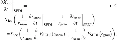
An important microphysical transfer term of ice phase chemical species was added for the sedimentation of grau-pel and snow, which contributes to wet deposition:
∂Xice
∂t
SEDI
= (14)
−Xice 1
rsnow
∂rsnow
∂t
SEDI + 1
rgrau
∂rgrau
∂t
SEDI
=Xice 1
rsnow
∂
∂zFSEDI(rsnow)+
1
rgrau
∂
∂zFSEDI rgrau
.
As shown in Table 4, 14 soluble chemical species and 5 intermediate ions have prognostic equations for the ice phase.
3 Application to idealized test cases
Three cases were run to assess the new module in Meso-NH. For all cases, the highly accurate PPM (piecewise parabolic method) scheme was used for the transport of the mete-orological and scalar fields. The first case, an idealized, warm, two-dimensional precipitating case, was used to study the sensitivity of the cloud chemistry to available warm cloud microphysical schemes. The second case, an idealized, mixed-phase, two-dimensional squall line, allowed us to as-sess the sensitivity of the cloud chemistry to the ice phase via the retention of chemical species when riming or freez-ing occurred. The last one, concernfreez-ing mixed-phase, three-dimensional supercells initialized with warm bubbles, was used to compare results with other CRMs, in particular the WRF-chem model (Barth et al., 2007b).
3.1 The HaRP case: a 2-D warm shallow convection case
54 1
2
Figure 1. HaRP case: time evolution of vertical profiles at the centre of the cloud cell for 3
mean raindrop radius (µm): (a) using the Kessler scheme and (b) using the C2R2 scheme. For 4
the Kessler scheme (a), the rain liquid water content (vol/vol) is superimposed as isolines. For 5
the C2R2 scheme (b), the number concentration of raindrops (L-1) is superimposed as 6
isolines. 7
8
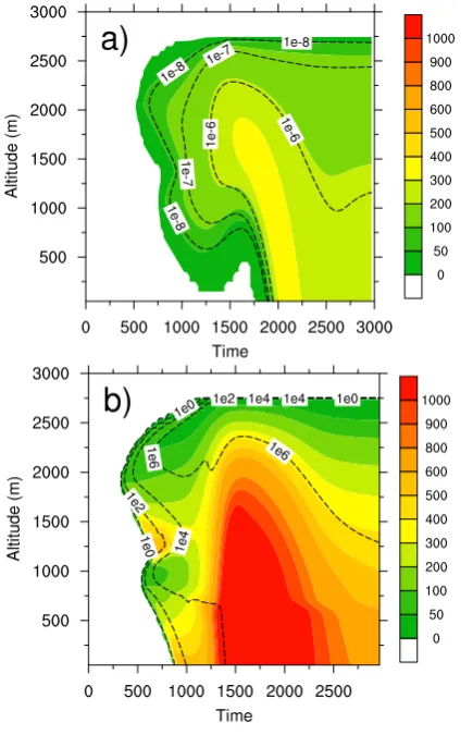
Fig. 1. HaRP case – time evolution of vertical profiles at the
cen-tre of the cloud cell for mean raindrop radius (µm): (a) using the Kessler scheme and (b) using the C2R2 scheme. For the Kessler scheme (a), the rain liquid water content (vol vol−1) is superim-posed as isolines. For the C2R2 scheme (b), the number concentra-tion of raindrops (L−1)is superimposed as isolines.
classical Kessler scheme, which is a one-moment scheme. The second one uses the C2R2 scheme, which includes a realistic parameterization of droplet nucleation described in Cohard et al. (1998). This parameterization is based on a four-parameter CCN activation spectrum taking into account the physicochemical properties of the accumulation mode in a natural aerosol population.
Cohard and Pinty (2000b) found numerous differences be-tween the Kessler and C2R2 simulations for the HaRP pre-cipitating cell. They found, after 1200 s of model simulation, that the rain began to reach the ground for the C2R2 case, unlike the Kessler case. At 1500 s of model simulation, they observed heavy precipitation at sea level for the C2R2 case while the Kessler case produced only a very sharp precipitat-ing band. After 1800 s of model simulation, the cell began to decay in the C2R2 case while it achieved a maximum devel-opment in the Kessler case. Very high radar reflectivity was observed for both cases at the end of the simulation. During
55 1
2
3
Figure 2.HaRP case: time evolution of vertical profiles at the centre of the cloud cell for 4
hydrogen peroxide mixing ratio (ppbv) in gas phase, in cloud water and in rainwater: (a) using 5
the Kessler scheme and (b) using the C2R2 scheme. Isoline of cloud liquid water content 6
(vol/vol, solid line) and of rain liquid water content (vol/vol, dashed line) are superimposed. 7
8
Fig. 2. HaRP case – time evolution of vertical profiles at the
cen-tre of the cloud cell for hydrogen peroxide mixing ratio (ppbv) in gas phase, in cloud water and in rainwater: (a) using the Kessler scheme and (b) using the C2R2 scheme. Isoline of cloud liquid wa-ter content (vol vol−1, solid line) and of rain liquid water content (vol vol−1, dashed line) are superimposed.
the course of the simulation, the rain water content was very high for the Kessler run with values up to 9×10⁻⁶vol vol−1, whereas the maximum value was 2.5×10⁻⁶vol vol−1 in C2R2 run. Cohard and Pinty (2000b) explained this differ-ence by the presdiffer-ence of an unrealistically small raindrop ra-dius with the Kessler scheme (Fig. 1).
The initial conditions for chemistry are shown in Table 5. These values correspond to a tropical marine atmosphere (Seinfeld and Pandis, 1998; Finlayson-Pitts and Pitts, 2000). Three different types of vertical profiles are allowed. For the “stratospheric vertical profile”, the initial mixing ratio is multiplied by 1 from 0 to 2 km and by 0.5 at 3 km. For the “boundary layer vertical profile”, the initial mixing ratio is multiplied by 1 from 0 to 1 km and by 0.1 from 2 to 3 km. Linear interpolation is used between values given at two lev-els. Simple DMS chemistry in gas phase, following Mari et al. (1999), is added to the ReLACS chemical scheme.
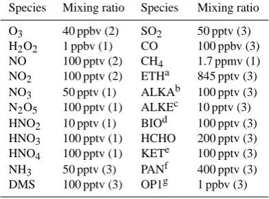
Table 5. Initial gas mixing ratios for the HaRP case. The form of the
vertical profile is indicated in parentheses as 1 for homogeneous, 2 for stratospheric, and 3 for boundary layer profile.
Species Mixing ratio Species Mixing ratio
O3 40 ppbv (2) SO2 50 pptv (3) H2O2 1 ppbv (1) CO 100 ppbv (3)
NO 100 pptv (2) CH4 1.7 ppmv (1)
NO2 100 pptv (2) ETHa 845 pptv (3)
NO3 50 pptv (1) ALKAb 100 pptv (3)
N2O5 100 pptv (1) ALKEc 10 pptv (3)
HNO2 10 pptv (1) BIOd 100 pptv (3)
HNO3 100 pptv (1) HCHO 200 pptv (3)
HNO4 100 pptv (1) KETe 100 pptv (3)
NH3 50 pptv (3) PANf 400 pptv (3)
DMS 100 pptv (3) OP1g 1 ppbv (3)
aETH=ethane;bALKA=alkanes other than methane and ethane, together with alkynes, alcohols, esters and epoxides;c
ALKE=anthropogenic alkenes;dBIO=biogenic species i.e. isoprene,α-pinene and d-limonene;eKET=acetone and higher saturated ketones;fPAN=Peroxyacetal nitrate and higher saturated PANs;gOP1=methyl hydrogen peroxide CH
3OOH.
SO2(aq)+HSO−3+SO 2−
3 . For hydrogen peroxide, which is
a soluble gas, it is easy to see the effect of wet deposition in the Kessler case (Fig. 2a). At the beginning of the simula-tion, hydrogen peroxide is scavenged by cloud water and then transferred to rain by microphysical conversion. The sedi-mentation of the raindrops and the simultaneous scavenging by raindrops lead to its efficient wet deposition. Moreover, during the course of the run, hydrogen peroxide is involved in the oxidation of sulphur dioxide leading to sulphuric acid. This is the main chemical sink of sulphur dioxide occurring in the liquid phase. Contrasting behaviour can be observed for the C2R2 case (Fig. 2b): the microphysical transfer from cloud water to rainwater is limited due to the two-moment approach in C2R2. Such a scheme is able to produce large raindrops in a reasonable concentration, thus with a mod-erate rainwater content (Fig. 1). Due to the large size of raindrops, the equilibrium time of the mass transfer between the gas phase and the aqueous phase is very long, leading to inefficient scavenging of hydrogen peroxide by raindrops (cf. Eq. 5). This is why the mixing ratio of hydrogen per-oxide in rainwater is limited inside the cloud, where col-lision/coalescence processes transfer chemical species from cloud water to rainwater. These processes are the main source of hydrogen peroxide inside raindrops for the C2R2 case. For sulphur dioxide, the same disparity can be observed between the Kessler and the C2R2 simulation. Additionally, the form of the initial vertical profile (boundary layer type) is visible (Fig. 3). Also, the mixing ratio of sulphur dioxide exceeds its initial value (50 pptv, see Table 5) in the low levels due to a production by DMS oxidation in the gas phase. Finally, its scavenging by cloud water is delayed compared to hy-drogen peroxide because of its lower solubility. Indeed, the
56 1
2
3
Figure 3. HaRP case: same as Figure 2 but for sulphur dioxide (pptv). 4
5 Fig. 3. HaRP case – same as Fig. 2 but for sulphur dioxide (pptv).
57 1
2
Figure 4. HaRP case: same as Figure 2 but for sulphuric acid in cloud water and in rainwater 3
(pptv). 4 5
Fig. 4. HaRP case – same as Fig. 2 but for sulphuric acid in cloud
water and in rainwater (pptv).
and H2O2mixing ratio in rain is very small; see Fig. 6) and
the production of sulphuric acid in rainwater is negligible. This simple idealized simulation highlights the role of the cloud microphysics scheme used in cloud chemistry. In par-ticular, using a two-moment scheme for cloud microphysics allows a better prediction of raindrop number concentration (Fig. 1), leading to a realistic mean raindrop diameter, which greatly changes the assessment of strong acid wet deposi-tion, as the temporal evolution of acid wet deposition rates is very sensitive to the values of raindrop radius. Another important point is the below-cloud aerosol particle scaveng-ing by rain, which is another significant source of strong acid wet deposition. This source is not considered here and should contribute mainly to the acidity of precipitation in a marine atmosphere, where aerosol particles are in the coarse mode, which is the mode more efficiently scavenged by falling rain-drops (Berthet et al., 2010.)
3.2 The COPT case: a 2-D tropical squall line
This case is built up from a tropical squall line observed in West Africa during the Convection Profonde Tropicale (COPT81) campaign on 23 June 1981. A tropical squall line is composed of two circulation features: a convective region and a stratiform region. The convective region is charac-terized by the mesoscale boundary layer convergence feed-ing deep convective updrafts and mid- to upper-level di-vergence associated with mass flux outflow from individ-ual cells. The stratiform region is characterized by mid-level convergence feeding both a mesoscale downdraft below the anvil and a mesoscale updraft within the stratiform part. The “COPT” test case (Caniaux et al., 1994) is typically a 12-hour simulation of a tropical squall line with kilometscale re-solved internal circulations, a 3-D turbulence scheme and
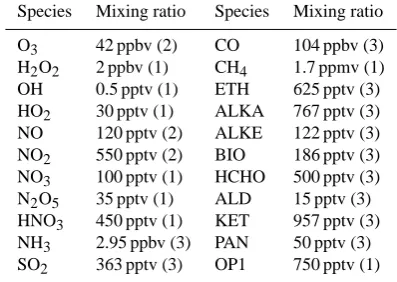
Table 6. Initial gas mixing ratios in the COPT case. The form of the
vertical profile is indicated in parentheses as 1 for homogeneous, 2 for stratospheric, and 3 for boundary layer profile.
Species Mixing ratio Species Mixing ratio
O3 42 ppbv (2) CO 104 ppbv (3) H2O2 2 ppbv (1) CH4 1.7 ppmv (1)
OH 0.5 pptv (1) ETH 625 pptv (3) HO2 30 pptv (1) ALKA 767 pptv (3)
NO 120 pptv (2) ALKE 122 pptv (3) NO2 550 pptv (2) BIO 186 pptv (3)
NO3 100 pptv (1) HCHO 500 pptv (3)
N2O5 35 pptv (1) ALD 15 pptv (3)
HNO3 450 pptv (1) KET 957 pptv (3)
NH3 2.95 ppbv (3) PAN 50 pptv (3) SO2 363 pptv (3) OP1 750 pptv (1)
mixed-phase microphysics (ICE3 scheme). The domain con-tains 320×44 grid points unevenly spaced in the vertical (z=70 m at ground level andz=700 m above 12 km). The horizontal resolution is 1.25 km. The model is integrated with a time step of 10 s. A gravity wave damping layer is inserted between 17 km and the model top at 22.5 km. A constant speed translation is used to compensate for the motion of the squall line. No fluxes are considered in the surface layer. Convection is initiated by forming a −0.01 K s−1 artificial cold pool in the low levels of a small domain for 10 min. Measurements available from the AMMA campaign (Stone et al., 2010) are used to build the initial profiles for chemical species. For unavailable species, the initial profiles are esti-mated either from simulation by the MOCAGE CTM model (Bousserez et al., 2007; Teyss´edre et al., 2007) at the lo-cation corresponding to the COPT campaign and for June; or from measurements averaged over June and July for the years 1998 to 2007 and taken from the IDAF database (Adon et al., 2010, http://idaf.sedoo.fr) at Lamto, Ivory Coast. In order to allow short-lived species with unknown concentra-tions to form and adjust their mixing ratios to an equilibrium state, a simulation with a box model corresponding to 24 h of spin-up was performed using the set of data composed by AMMA and IDAF measurements as initial conditions, as well as MOCAGE simulation results. The resulting initial mixing ratios in the boundary layer for the COPT case are indicated in Table 6. For the “stratospheric vertical profile”, the initial mixing ratio is multiplied by 1 from 0 to 2 km, by 0.5 from 3 to 13 km, by 0.75 at 14 km and by 1 at 15 km. For the “boundary layer vertical profile”, the initial mixing ratio is multiplied by 1 from 0 to 1 km, by 0.1 from 2 to 13 km and by 0.05 from 14 km to 15 km. Linear interpolation is used between values given at two levels.
58 1
2
Figure 5. HaRP case: time evolution of vertical profiles at the centre of the cloud cell for pH 3
value in rainwater: (a) using the Kessler scheme, and (b) using the C2R2 scheme. The rain 4
liquid water content (vol/vol) is superimposed as isolines. 5
6
Fig. 5. HaRP case – time evolution of vertical profiles at the centre
of the cloud cell for pH value in rainwater: (a) using the Kessler scheme, and (b) using the C2R2 scheme. The rain liquid water con-tent (vol vol−1) is superimposed as isolines.
assuming that mixing ratios of soluble species in the liquid phase are fully transferred to the gas phase when freezing or riming occurs, which corresponds to RET=0 for all species. The third one (AQ-ICE) considers the retention of soluble chemical species in the precipitating ice hydrometeors, i.e. prognostic scalar variables are considered for the mixing ra-tio of soluble species in ice. Results will be shown in the following as averages obtained between 7 and 8 h of simula-tion and corresponding to the mature stage of the squall line (Caniaux et al., 1994), which is characterized by a convective zone 40 km wide giving large precipitation, a well developed stratiform zone stretching over 150 km and giving moderate precipitation over an area 80 km wide, and a forward anvil at the tropical easterly jet level near 12 km.
In this section, we focus on three chemical species with in-creasing solubility and retention coefficient in the ice phase: formaldehyde HCHO, formic acid HCOOH and sulphuric acid H2SO4.
The budget of formaldehyde in the upper troposphere (UT) is still uncertain although HCHO is a potentially significant
59 1
Figure 6. HaRP case: time evolution of the mixing ratio below the cloud (250 m above sea 2
level) for hydrogen peroxide in gas phase and in rainwater (left), for sulphur dioxide in gas 3
phase and in rainwater, and for sulphuric acid in rainwater (right) for both cases: Kessler 4
(black lines) and C2R2 (grey lines). 5
6
Fig. 6. HaRP case – time evolution of the mixing ratio below the
cloud (250 m a.s.l.) for hydrogen peroxide in gas phase and in rain-water (left); and for sulphur dioxide in gas phase and in rainrain-water, and for sulphuric acid in rainwater (right) for both cases: Kessler (black lines) and C2R2 (grey lines).
source of HOx via its photolysis in the UT (Cohan et al.,
1999). HCHO observed in the UT is due to direct transfer of boundary layer HCHO and chemical secondary produc-tion by transported VOCs. Fried et al. (2008) and Stickler et al. (2006) showed an HCHO enhancement in the convective outflow for summertime deep convection over North Amer-ica and the North Atlantic, and in the middle and upper tro-posphere over Europe, respectively. Borbon et al. (2012) ob-served a moderate enhancement of HCHO in the convective outflow for a mesoscale convective system over West Africa. Fried et al. (2008) and Borbon et al. (2012) estimated that 70 % and 60 %, respectively, of the HCHO observations in the UT after convection were related to an enhanced produc-tion from precursors rather than an upward transport from the boundary layer.
60 1
Figure 7. COPT case: simulated mixing ratio of formaldehyde during the mature stage of the 2
squall line: a) simulated gas phase mixing ratio of HCHO for the GAS simulation, b) 3
simulated total mixing ratio of HCHO (gas + cloud water + rainwater) for the AQ-NOICE 4
simulation, c) simulated total mixing ratio of HCHO (gas + cloud water + rainwater + 5
precipitating ice) for the AQ-ICE simulation, and d) simulated mixing ratio of HCHO in 6
precipitating ice for the AQ-ICE simulation. The black line is the 0.01 g/kg isoline cloud 7
water mixing ratio, the purple line is that for precipitating ice (snow + graupel) and the mauve 8
is that for rainwater. 9
10
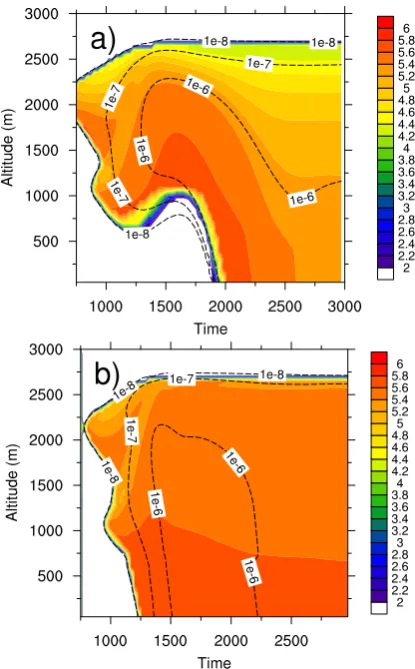
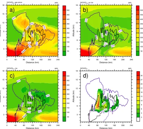
Fig. 7. COPT case – simulated mixing ratio of formaldehyde during
the mature stage of the squall line: (a) simulated gas phase mixing ratio of HCHO for the GAS simulation, (b) simulated total mixing ratio of HCHO (gas+cloud water+rainwater) for the AQ-NOICE simulation, (c) simulated total mixing ratio of HCHO (gas+cloud water+rainwater+precipitating ice) for the AQ-ICE simulation, and (d) simulated mixing ratio of HCHO in precipitating ice for the AQ-ICE simulation. The black line is the 0.01 g kg−1isoline cloud water mixing ratio, the mauve line is that for precipitating ice (snow +graupel), and the purple is that for rainwater.
is observed in the forward anvil and in the stratiform part of the cloud, while it falls below 150 pptv for the AQ-NOICE case. The comparison between the two simulations including cloud chemistry (Fig. 7b and c) is interesting: for AQ-ICE case (Table 4, RET=0.64 for HCHO), values of HCHO in the anvil and in the stratiform part of the cloud are very low, less than 100 pptv with some areas having values less than 50 pptv. The mixing ratio of HCHO in the ice phase during the mature stage of the cloud is less than 30 pptv (Fig. 7d), so alone it cannot explain the difference between Fig. 7b and c. Along the squall line development, the HCHO in the ice phase is partly eliminated by rain due to the melting of snow and graupel during their sedimentation. This is the main rea-son for the depletion of HCHO in the gas phase in the UT observed in the AQ-ICE simulation. Non-soluble precursors of HCHO, such as ETH and ALK ReLACS species (respec-tively ethane and alkanes other than methane and ethane, to-gether with alkynes, alcohols, esters and epoxides), are trans-ported in a similar way to CO in the forward anvil, the strati-form part of the cloud and the convective outflow. However, their contribution to the HCHO mixing ratio in the UT is very small, as shown by the comparison between Fig. 7c and a. No signature of a secondary production of HCHO in the UT is observed for the AQ-ICE case. In conclusion, the effect of the retention of HCHO in ice is to enhance its scavenging
61 1
Figure 8. COPT case: vertical profiles of gas phase mixing ratio of formaldehyde: black lines 2
are mixing ratio for GAS (dashed line), AQ-NOICE (dotted line) and AQ-ICE (solid line) 3
simulations and the solid grey line is the mixing ratio for the background troposphere, (a) in 4
the inflow region (20 km in horizontal distance) of the squall line during its mature stage, (b) 5
in the outflow region (200 km in horizontal distance) of the squall line during its mature 6
stage. 7 8
Fig. 8. COPT case – vertical profiles of gas phase mixing ratio
of formaldehyde: black lines are mixing ratio for GAS simula-tion (dashed line), AQ-NOICE simulasimula-tion (dotted line) and AQ-ICE simulation (solid line), for simulations, and the solid grey line is the mixing ratio for the background troposphere (a) in the inflow region (20 km in horizontal distance) of the squall line during its mature stage and (b) in the outflow region (200 km in horizontal distance) of the squall line during its mature stage.
In conclusion, the vertical profile of HCHO in the outflow region for the AQ-ICE simulation compares well with the vertical profile given in Fig. 6 of Borbon et al. (2012) study.
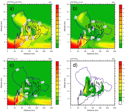
Results from global model predict that formic acid origi-nates primarily from the photo-oxidation of biogenic com-pounds. However, there is still a large uncertainty in the sources of formic acid. To reconcile simulated and observed formic acid mixing ratios, Paulot et al. (2011) reported ev-idence for a long-lived missing secondary source of car-boxylic acids that may be associated with the aging of or-ganic aerosols. In Barth et al. (2007b), formaldehyde was the major precursor of formic acid in the aqueous phase, which was a good tracer of cloud-processed air since its sources in the gas phase are low. Formic acid is a secondary species, both in gas- and aqueous phases. In the gas phase, formic acid is mainly produced in the ReLACS mechanism by the ozonolysis of alkenes (ALKE species in ReLACS) and of biogenic VOC (BIO species in ReLACS). In the aqueous phase, it is produced by the oxidation of hydrated formalde-hyde by OH radical (Table 3). Its main destruction pathway is oxidation by OH in either the gas or aqueous phase. No formic acid is present initially. As for formaldehyde, a gas phase production is observed in the front of the squall line (Fig. 9a–c). However, in contrast to HCHO production, the maximum of HCOOH mixing ratio for the GAS simulation is about 10.5 pptv, whereas it is about 11.6 pptv for the AQ-NOICE and AQ-ICE cases. This difference is due to a small contribution of aqueous phase chemistry to the gas phase mixing ratio in the front of the squall line. Although a greater production of formic acid via aqueous phase chemistry was expected (the initial mixing ratio of its main precursor in aqueous phase is 500 pptv in the boundary layer), results ac-tually show a very small contribution of cloud reactivity in the net production of formic acid. This is partly explained by the destruction of formate ion by OH in the aqueous phase, which is more efficient than the oxidation of formic acid by OH (Table 3). This pathway dominates due to high pH val-ues in cloud water and rainwater (pKa(formic acid)=3.75 at 298 K; Table 2). Values of pH were between 6 and 6.5 (not shown) due to a very high mixing ratio of ammonia (almost 3 ppbv in the boundary layer, see Table 6) and low mixing ra-tio of sulphur dioxide. The effect of the retenra-tion of HCOOH in ice is the same as simulated for HCHO with a depletion of formic acid in the UT (Fig. 9c), which cannot be directly explained by its amount in ice precipitating hydrometeors (Fig. 9d). Barth et al. (2007) found a HCOOH production of about 100 pptv in the core of the storm where the cloud water is located, whereas, in the COPT case, this production is very low, a few pptv. Two main differences between Barth et al. (2007) and the COPT case in our study explain this discrepancy. First, in Barth et al. (2007), the initial mixing ratio of HCHO, the precursor of HCOOH in aqueous phase, was about 2 ppbv at the surface, whereas it is 500 pptv in the COPT case. Secondly, in the COPT case, the pH value in cloud water is high, between 6 and 6.5 whereas it was around
62 1
Figure 9. COPT case: same as Figure 7 but for formic acid. 2
3
Fig. 9. COPT case – same as Fig. 7 but for formic acid.
4.5 in the simulation of Barth et al. (2007). Thus, the destruc-tion of formic acid is more efficient in our study because the formate ion pathway dominates at high pH value.
63 1
Figure 10. COPT case: same as Figure 7 but for sulphuric acid. 2
3 Fig. 10. COPT case – same as Fig. 7 but for sulphuric acid.
cell evolves in a squall line. As already pointed out for formic acid, the AQ-ICE simulation shows a very low mixing ratio of soluble species (here sulphuric acid) inside the forward anvil and the stratiform part of the squall line (Fig. 10d) due to efficient trapping of soluble species inside the ice-precipitating hydrometeors, then contributing to wet depo-sition.
For this particular simulation, the results show that the ef-fect of the retention of soluble species in the ice phase is to enhance the scavenging efficiency of soluble species and thus to increase the wet deposition of the soluble species. This is consistent with the very high accumulated precipitation due to melting of snow and graupel in the convective part of the cloud.
3.3 The STERAO case: a 3-D continental storm
The STERAO (Stratospheric-Tropospheric Experiment: Ra-diation, Aerosol, and Ozone) convective system observed on 10 July 1996 took place near the southern border of Wyoming and Nebraska (see Dye et al., 2000 for an overview of the experiment). The storm developed during the late af-ternoon, the main cells propagated south-south-eastward into north-eastern Colorado before dissipating in the evening. Radar reflectivity observations showed an evolution of the storm from a multicell stage followed by a quasi supercel-lular one (Dye et al., 2000). The simulation of this storm performed with the Meso-NH model is a 3-D idealized run based upon Skamarock et al. (2000) with some modifica-tions. The convection is initiated with three warm bubbles (+3◦C) placed in the wind direction leading to a simulated convective system similar to the one observed. In particular, the transition from a multicellular line to a single supercell
is reproduced. The configuration of the model is the same as in Barthe et al. (2012). A 160×160 km2 horizontal do-main is used with a 1 km horizontal resolution. The verti-cal grid has 51 levels up to 23 km with a level spacing of 50 m close to the surface, stretching to 700 m at the top of the domain. The terrain height is 1.5 km. The time step is 2.5 s and the simulation lasts for 3 h. For cloud microphysics, the mixed-phase scheme ICE3 is used and, for turbulence, the 3-D scheme is activated. A simple module for the parameter-ization of the NO production from lightning is used, follow-ing Pickerfollow-ing et al. (1998). However, the production of NO by cloud-to-ground flash and intracloud flash are taken from Barth et al. (2007b). Based upon observations and model results, Barth et al. (2007b) estimated that each cloud-to-ground flash produced 390 moles of NO on average and an intracloud flash, 195 moles of NO on average. The model en-vironment is initialized with horizontally homogeneous ther-modynamic sounding and chemical vertical profiles. These initial vertical profiles for chemical species (O3, NO, NO2,
NH3, HNO3, CO, CH4, HCHO, H2O2, CH3OOH and SO2)
were given in Barth et al. (2007a, b) and were estimated from aircraft measurements outside the cloud. VOC precursors of HCHO, apart from methane, are not considered in this simu-lation.
Results are evaluated in comparison with the simulation reported in Barth et al. (2007b), with particular focus on a comparison of simulations considering or ignoring the re-tention of soluble species in ice precipitating hydrometeors. In Barth et al.’s (2007b) study, the WRF-Chem model was used in a configuration close to Meso-NH. The main differ-ences between the two models lay in the chemical mecha-nism and the parameterization of cloud ice phase chemistry. In Barth et al. (2007b), the chemical mechanism predicted the mixing ratio of 16 species and was limited to the chem-istry of an ozone-NOx-HOx-CH4-SO2system with 28
chem-ical reactions in the gas phase, the exchange of 16 species between gas- and aqueous phases and 15 reactions in the aqueous phase. In the aqueous phase, the reactivity of NOy
species was not considered. For the interaction with the ice phase of the cloud, two simulations were performed in Barth et al. (2007b): either dissolved species were completely re-tained in the ice phase when cloud droplets, or raindrops froze (RET=1) or all dissolved species were degassed dur-ing freezdur-ing (RET=0).
As shown in Barth et al. (2007b), CO is transported from the boundary layer to the anvil of the cloud where mixing ra-tios are>110 ppbv, greater than the unperturbed UT at the same level (Fig. 11a and b). As in Barth et al. (2007b), the comparison of CO and ozone with measurements across the anvil are in good agreement (not shown). Results are now dis-cussed for HCHO and H2O2, two soluble and reactive gases.
For HCHO, the results are shown at 1 h, corresponding to the multicell stage of the cloud.
64 1
Figure 11. STERAO case: results at t = 3600 s for (a) horizontal cross section of CO mixing 2
ratio in ppbv at 10 km a.g.l., (b) vertical cross section along the segment indicated on (a) for 3
CO mixing ratio in ppbv, (c) same vertical cross section for HCHO total mixing ratio (gas + 4
cloud water + rainwater + precipitating ice) in pptv for simulation with retention in ice, (d) 5
same as (c) for simulation without retention in ice, (e) same vertical cross section for the ratio 6
of total HCHO to CO in pptv/ppbv for simulation with retention in ice, (f) same as (e) for 7
simulation without retention in ice. 8
9
Fig. 11. STERAO case – results att=3600 s for (a) horizontal cross section of CO mixing ratio in ppbv at 10 km a.g.l., (b) vertical cross section along the segment indicated on (a) for CO mixing ra-tio in ppbv, (c) same vertical cross secra-tion for HCHO total mixing ratio (gas+ cloud water+rainwater+precipitating ice) in pptv for simulation with retention in ice, (d) same as (c) for simulation without retention in ice, (e) same vertical cross section for the ratio of total HCHO to CO in pptv ppbv−1for simulation with retention in ice, and (f) same as (e) for simulation without retention in ice.
layer to the anvil (Fig. 11c and d) during the multicell stage of the cloud. However, the total mixing ratio of HCHO in the anvil is greater for the simulation considering retention in ice (Fig. 11c) than in the one with no retention (Fig. 11d). HCHO and CO have the same initial vertical profile but with different magnitudes. It is thus interesting to compare the re-distribution by the cloud of HCHO, a soluble and reactive species, and that of CO, an insoluble passive species. Con-sistently with results for the total mixing ratio of HCHO, the ratio of total HCHO to CO shows a transport of HCHO from the boundary layer to the anvil, which is efficient in the sim-ulation with retention in ice. The ratio of total HCHO to CO also reveals that vertical transport inside the cloud is less ef-ficient for HCHO than for CO, indicating that a fraction of HCHO has reacted or precipitated to the ground. This effect described in Barth et al. (2007b) is similar. Looking at the gas phase mixing ratio of HCHO (Fig. 12a and b), the simulated
65 1
Figure 12. STERAO case: results at t = 3600 s for vertical cross section of HCHO mixing 2
ratio in pptv along the segment indicated on Fig. 10a, at the left hand side for simulation with 3
retention in ice and at the right hand side for simulation without retention: (a) and (b) in gas 4
phase, (c) and (d) in cloud water, (e) and (f) in rainwater, (g) in precipitating ice. The black 5
line represents the total hydrometeors mixing ratio equal to 0.01 g/kg, the mauve line on (c) 6
Fig. 12. STERAO case – results att=3600 s for vertical cross sec-tion of HCHO mixing ratio in pptv along the segment indicated in Fig. 10a, left hand side, for simulation with retention in ice, and right hand side for simulation without retention: (a) and (b) in gas phase, (c) and (d) in cloud water, (e) and (f) in rainwater, and (g) in precipitating ice. The black line represents the total hydromete-ors mixing ratio equal to 0.01 g kg−1, the grey line in (c) and (d) is the same for cloud water, the grey line in (e) and (f) is the same for rainwater, and the grey line in (g) is the same for precipitating ice.
67 1
Figure 13. STERAO case: vertical profiles of gas phase mixing ratio of formaldehyde: black 2
lines are mixing ratio in the convective outflow (135 km in horizontal distance in reference to 3
Fig. 12a, b) for simulation with retention in ice (solid line) and for simulation without 4
retention (dotted line). The solid grey line is the mixing ratio for the unperturbed troposphere. 5
Fig. 13. STERAO case – vertical profiles of gas phase mixing
ra-tio of formaldehyde: black lines are mixing rara-tio in the convective outflow (135 km in horizontal distance in reference to Fig. 12a and b) for simulation with retention in ice (solid line), and for simula-tion without retensimula-tion (dotted line). The solid grey line is the mixing ratio for the unperturbed troposphere.
retention, HCHO degasses when freezing occurs, and is ab-sorbed subsequently by the supercooled cloud water at the top of the updraft. This result was already found by Barth et al. (2001) in their simulation with no retention for all sol-uble trace gases. In comparison to Barth et al. (2007b), the same order of magnitude is retrieved for the HCHO mixing ratio in cloud water but lower values are observed in rain-water. In Barth et al. (2007b), the mixing ratios of soluble species were explicitly represented in each of the ice phase hydrometeor categories. However, the comparison of the sum of HCHO mixing ratios in snow and in hail categories from Barth et al. (2007b) with the HCHO mixing ratio in precipi-tating ice from our simulation (Fig. 12g) shows the same or-der of magnitude. Thus, the global approach for the ice phase species mixing ratio representation used in Meso-NH seems to be comparable to a more explicit approach. The main gen-eral remarks concern results of HCHO mixing ratio during the supercell stage of the cloud (after 2.5 h of simulation). In particular, the depletion of gas phase mixing ratio of HCHO in the convective outflow is again observed for the simula-tion with retensimula-tion in ice, whereas the simulasimula-tion without retention shows enrichment in the anvil (not shown). This difference is due to the capture of HCHO in the ice phase. The greater value of total HCHO mixing ratio observed for the simulation with retention in ice whatever the stage of the storm in comparison to simulation without retention indi-cates the formation of a reservoir of HCHO in the ice phase in the simulation with retention in ice, leading to less HCHO remaining available to react in the gas- and aqueous phases.
68 1
Figure 14. STERAO case: results at t = 3600 s for vertical cross section of H2O2 mixing ratio 2
in pptv along the segment indicated on Fig. 10a, on the left hand side for simulation with 3
retention in ice and on the right hand side for the simulation without retention: (a) and (b) 4
total mixing ratio, (c) and (d) in gas phase. The black line represents the total hydrometeors 5
mixing ratio equal to 0.01 g/kg. 6
7
Fig. 14. STERAO case – results att=3600 s for vertical cross sec-tion of H2O2mixing ratio in pptv along the segment indicated in
Fig. 10a, left hand side, for simulation with retention in ice, and right hand side for the simulation without retention: (a) and (b) total mixing ratio, and (c) and (d) in gas phase. The black line represents the total hydrometeors mixing ratio equal to 0.01 g kg−1.
The same effect is observed for hydrogen peroxide (Fig. 14a and b). Moreover, as hydrogen peroxide is more soluble than HCHO in liquid water and is very reactive in aqueous phase with sulphur dioxide, its vertical transport from the boundary layer to the anvil is less efficient than for HCHO. A significant depletion is observed in the convective cores for hydrogen peroxide in gas phase for the simulation with retention in ice (Fig. 14c), underlying its capture in the ice phase. This depletion is also observed for the simulation without retention in ice (Fig. 14d), whereas this effect is not observed for HCHO (Fig. 12b). This difference stems from the very efficient transfer of hydrogen peroxide from the gas phase to the liquid phase due to its high reactivity and its high solubility in the aqueous phase.
As in Barth et al. (2007b), integrated results are shown as percentages of HCHO and H2O2in each water chemical