Geosci. Model Dev., 6, 883–899, 2013 www.geosci-model-dev.net/6/883/2013/ doi:10.5194/gmd-6-883-2013
© Author(s) 2013. CC Attribution 3.0 License.
EGU Journal Logos (RGB)
Advances in
Geosciences
Open Access
Natural Hazards
and Earth System
Sciences
Open AccessAnnales
Geophysicae
Open AccessNonlinear Processes
in Geophysics
Open AccessAtmospheric
Chemistry
and Physics
Open AccessAtmospheric
Chemistry
and Physics
Open Access DiscussionsAtmospheric
Measurement
Techniques
Open AccessAtmospheric
Measurement
Techniques
Open Access DiscussionsBiogeosciences
Open Access Open Access
Biogeosciences
DiscussionsClimate
of the Past
Open Access Open Access
Climate
of the Past
Discussions
Earth System
Dynamics
Open Access Open Access
Earth System
Dynamics
DiscussionsGeoscientific
Instrumentation
Methods and
Data Systems
Open Access
Geoscientific
Instrumentation
Methods and
Data Systems
Open Access DiscussionsGeoscientific
Model Development
Open Access Open Access
Geoscientific
Model Development
DiscussionsHydrology and
Earth System
Sciences
Open AccessHydrology and
Earth System
Sciences
Open Access DiscussionsOcean Science
Open Access Open Access
Ocean Science
Discussions
Solid Earth
Open Access Open Access
Solid Earth
DiscussionsThe Cryosphere
Open Access Open Access
The Cryosphere
Discussions
Natural Hazards
and Earth System
Sciences
Open Access
Discussions
Evaluation of dust and trace metal estimates from the Community
Multiscale Air Quality (CMAQ) model version 5.0
K. W. Appel1, G. A. Pouliot1, H. Simon2, G. Sarwar1, H. O. T. Pye1, S. L. Napelenok1, F. Akhtar3, and S. J. Roselle1 1Atmospheric Modeling and Analysis Division, National Exposure Research Laboratory,
Office of Research and Development, US Environmental Protection Agency, Research Triangle Park, North Carolina, USA 2Air Quality Assessment Division, Office of Air Quality Planning and Standards, Office of Air and Radiation,
US Environmental Protection Agency, Research Triangle Park, North Carolina, USA
3Heath and Environmental Impacts Division, Office of Air Quality Planning and Standards, Office of Air and Radiation, US Environmental Protection Agency, Research Triangle Park, North Carolina, USA
Correspondence to: K. W. Appel ([email protected])
Received: 30 January 2013 – Published in Geosci. Model Dev. Discuss.: 7 March 2013 Revised: 10 May 2013 – Accepted: 31 May 2013 – Published: 4 July 2013
Abstract. The Community Multiscale Air Quality (CMAQ) model is a state-of-the-science air quality model that simu-lates the emission, transformation, transport, and fate of the many different air pollutant species that comprise particu-late matter (PM), including dust (or soil). The CMAQ model version 5.0 (CMAQv5.0) has several enhancements over the previous version of the model for estimating the emission and transport of dust, including the ability to track the specific elemental constituents of dust and have the model-derived concentrations of those elements participate in chemistry. The latest version of the model also includes a parameteri-zation to estimate emissions of dust due to wind action. The CMAQv5.0 modeling system was used to simulate the entire year 2006 for the continental United States, and the model es-timates were evaluated against daily surface-based measure-ments from several air quality networks. The CMAQ mod-eling system overall did well replicating the observed soil concentrations in the western United States (mean bias gen-erally around±0.5 µg m−3); however, the model consistently overestimated the observed soil concentrations in the eastern United States (mean bias generally between 0.5–1.5 µg m−3), regardless of season. The performance of the individual trace metals was highly dependent on the network, species, and season, with relatively small biases for Fe, Al, Si, and Ti throughout the year at the Interagency Monitoring of Pro-tected Visual Environments (IMPROVE) sites, while Ca, K, and Mn were overestimated and Mg underestimated. For the urban Chemical Speciation Network (CSN) sites, Fe, Mg,
and Mn, while overestimated, had comparatively better per-formance throughout the year than the other trace metals, which were consistently overestimated, including very large overestimations of Al (380 %), Ti (370 %) and Si (470 %) in the fall. An underestimation of nighttime mixing in the ur-ban areas appears to contribute to the overestimation of trace metals. Removing the anthropogenic fugitive dust (AFD) emissions and the effects of wind-blown dust (WBD) low-ered the model soil concentrations. However, even with both AFD emissions and WBD effects removed, soil concentra-tions were still often overestimated, suggesting that there are other sources of errors in the modeling system that contribute to the overestimation of soil components. Efforts are under-way to improve both the nighttime mixing in urban areas and the spatial and temporal distribution of dust-related emission sources in the emissions inventory.
1 Introduction
and/or reflecting solar radiation (Sokolik and Toon, 1996). As such, understanding the emission, transport and fate of dust in the environment is important for protecting human health and sensitive ecosystems, as well as assessing the im-pact of air quality on climate (e.g., surface temperature) due to radiative feedbacks from dust and PM.
The Community Multiscale Air Quality (CMAQ; Byun and Schere, 2006) model is a state-of-the-science air quality model capable of reproducing the emission, transformation, transport, and fate of the many different air pollutant species that comprise PM, including dust. The latest release of the CMAQ model, version 5.0 (CMAQv5.0), includes several enhancements over the previous version of the model (ver-sion 4.7; Foley et al., 2011) for estimating the emis(ver-sion and transport of dust. Specifically, the model now includes the ability to explicitly track the specific elemental constituents of dust (e.g., silicon, calcium, iron, etc.) and where applica-ble, have the model-derived concentration of those elements participate in the model chemistry. Previous versions of the model used prescribed “background” values for several ele-ments and therefore did not represent the spatial and seasonal variations in the concentrations of those elements. The lat-est version of the model also includes a parameterization for estimating the emission of dust due to wind action (wind-blown dust; WBD). In addition, the emission inputs have been updated to include sources of anthropogenic fugitive dust (AFD), such as dust from unpaved roads and agricultural tilling, and the chemical boundary conditions (BCs) now in-clude WBD from long-range transport.
In this study, the CMAQv5.0 model has been used to sim-ulate the entire year 2006 for the continental United States (CONUS). The CMAQ model estimates of the trace elements comprising dust are evaluated against daily surface-based measurements of the same elements. In addition to the annual base simulation, several seasonal sensitivity simulations are performed in order to assess the impact that changes made to the emissions inventory, boundary conditions, and inclusion of the WBD mechanism have on the CMAQ model estimates of dust. Finally, several recommendations for further improv-ing the CMAQ estimates of dust are discussed.
2 Model inputs and configuration
The CMAQ model requires inputs of gridded meteorolog-ical fields, emissions data, and boundary conditions. For a regional or continental CMAQ model simulation, the mete-orological fields are typically provided by a regional scale meteorological model, such as the Weather Research and Forecast (WRF; Skamarock et al., 2008) model. The input emissions are typically derived from a standard emissions input database, such as the USEPA’s National Emissions In-ventory (NEI), for which base year inventories are avail-able every three years. Finally, chemical boundary condi-tions are typically based off a larger, coarser CMAQ model
simulation or from a hemispheric or global air quality simu-lation provided by a global chemistry model. The meteoro-logical, emission, and boundary condition inputs used in the base CMAQ model simulation are described in this section.
2.1 Meteorological inputs
The meteorological inputs for the CMAQ model simula-tions were provided by a 2006 annual CONUS WRFv3.3 model simulation that utilized 12 km horizontal grid spac-ing and 35 vertical layers of variable thickness extendspac-ing up to 50 hPa, with the top of the lowest model layer at ap-proximately 20 m above ground level. Initial and boundary conditions for WRF were provided by the North American Mesoscale Model (NAM) available from the National Cen-ters for Environmental Prediction. The WRF simulation uti-lized the Rapid Radiation Transfer Model Global (RRTMG) for long- and short-wave radiation (Iacono et al., 2008), the Kain–Fritsch 2 cumulus parameterization (Kain, 2004), the Morrison microphysics scheme (Morrison et al., 2009), the Pleim–Xiu land-surface model (PX-LSM; Xiu and Pleim, 2001; Pleim and Xiu, 1995), and the Asymmetric Convec-tive Model version 2 (ACM2; Pleim, 2007a and b) planetary boundary layer (PBL) scheme.
Four-dimensional data assimilation (FDDA) was used to constrain the model above the PBL; however unlike previ-ous WRF model simulations, no FDDA was used within the PBL, which results in an improved wind speed bias in the PBL as compared to WRF simulations that utilized FDDA throughout the troposphere (Gilliam et al., 2012). The raw WRF outputs were processed for the CMAQ model using version 4.0 of the Meteorology-Chemistry Interface Proces-sor (MCIP; Otte and Pleim, 2010). A 10-day spin-up period was utilized to eliminate the effects of the initial conditions, while the simulation was run in 5- and half-day increments with 12 h overlaps between segments.
2.2 Emission inputs
2.2.1 Base emissions
in-line in CMAQ and are based on the Biogenic Emissions Inventory System (BEIS) v3.14 (http://www.cmascenter. org). Mobile emissions were calculated for 2006 using the MOBILE6 vehicle emission modeling software (http://www. epa.gov/oms/m6.htm). For the remaining source sectors (i.e., area sources and non-EGU point sources) the emission esti-mates in the 2005 NEI are the same as the 2002 version of the NEI. Wind-blown dust and lightning NOX(NO+NO2) (Allen et al., 2012) were calculated using time-dependent in-put meteorology and observations from the National Light-ning Detection Network (NLDN). The raw emissions inputs were preprocessed for the CMAQ model using the Sparse Matrix Operator Kernel Emissions (SMOKE; Houyoux et al., 2000).
2.2.2 Anthropogenic fugitive dust emissions
Crustal elements such as Ca and Fe are present in anthro-pogenic and wind-blown fugitive dust, but may also be found in some fly ash and industrial process emissions (which are chemically similar to crustal emissions). The sources of AFD include unpaved road dust, paved road dust, commercial con-struction, residential concon-struction, road concon-struction, agricul-tural tilling, livestock operations, and mining and quarry-ing. Unpaved road dust is the largest single emission cate-gory within the non-point fugitive dust catecate-gory, accounting for about one-third of non-windblown fugitive dust emis-sions. This is followed in size by dust from tilling, quarry-ing, and other earthmoving. Source apportionment studies have shown that AFD emissions contribute on the order of 5–20 % of PM2.5and 40–60 % of PM10in urban areas that ei-ther have been or potentially may be unable to attain the Na-tional Ambient Air Quality Standards (NAAQS) for PM2.5 and/or PM10(Watson and Chow, 2000). Conversely, air qual-ity models suggest vastly higher contributions from current fugitive dust emission inventories, with contributions ranging from 50 to 80 % for PM2.5and 70 to 90 % for PM2.5and/or PM10 (Watson and Chow, 2000). Although dust makes up the majority of PM emissions, much of the emitted mass gets deposited on surfaces near the source at scales much smaller than the model grid-cell resolution (Veranth et al., 2003; Etyemezian et al., 2004). This is not true of other sources that are either emitted at a higher elevation (e.g., power plant stacks) or are emitted in warm exhaust (e.g., from vehicles) that rises quickly and gets entrained into the air mass. To correct for the near-source removal of dust, emissions from these sources are typically multiplied by a transportable frac-tion as proposed by Pace (2005). This transportable fracfrac-tion is applied on a per county basis to both PM10and PM2.5.
PM2.5emissions in the NEI are reported as an annual total. In order for these emissions to be used in modeling applica-tions, they need to be chemically speciated and allocated to finer temporal resolutions (e.g., each hour of the year). PM2.5 emissions in the NEI are typically speciated into five chem-ical components (organic carbon (OC), elemental carbon
(EC), sulfate, nitrate, and other). Recently, an improved spe-ciation of the PM has been developed to include, in addi-tion to the current PM species, a range of trace metals as well as separate non-carbon organic matter and metal-bound oxygen (Reff et al., 2009). The current temporal profile used by the EPA to allocate dust emissions to daily resolution as-sumes no monthly variability and no weekday/weekend vari-ation (http://www.epa.gov/ttn/chief/emch/index.html#2005). In essence, each day is represented identically throughout the year. Additional, emissions from AFD sources are set to zero for any hour or in any grid cell when there is snow cover or when the soil is at least 50 % saturated in the first 1 cm depth based on the soil types and saturation values in the PX-LSM. In this work, three changes were made to improve and di-agnose the fugitive dust emission estimates used in chemical transport modeling. The first change involves improvements to the transportable fraction applied to the gridded emission inventory field. Second, a new mapping of the temporal pro-files is applied to fugitive dust emissions so that they vary by day of the year. Finally, the chemical speciation of PM2.5 emissions is updated based on Reff et al. (2009). This allows for better source attribution of the measured trace metals.
In Pace (2005), the transportable fraction, (i.e., the frac-tion of total mass that is not “captured” by near-source re-moval), is calculated on a per county basis for three regional planning organizations using the BEIS version 2 county-level land use information (Byun and Ching, 1999). To improve the transportable fraction in CMAQ, it was recalculated at a 1 km resolution using the newer BELD3 database (Vukovich and Pierce, 2002) for all of the CONUS using five broad land use categories (e.g., forest, urban, sparsely wooded and grass, agricultural, and barren/water), generally resulting in an increase in the transportable fraction in the western United States and little change to the transportable fraction in the eastern United States (Pouliot et al., 2010). Table 1 shows the mapping of the BELD3 land use types to the five broad land use categories and the associated capture fraction.
Table 1. BELD3 categories, capture fraction class, and trans-portable fraction. Transtrans-portable fraction (ranging from 0 to 1) is defined as the fraction of total emitted PM mass that becomes en-trained in the grid-cell mass.
BELD3 Capture Transportable
Category Fraction Class Fraction
USGS urban Urban 0.50
USGS drycrop Grass 0.75
USGS irrcrop Grass 0.75
USGS cropgrass Grass 0.75
USGS cropwdlnd Grass 0.75
USGS grassland Grass 0.75
USGS shrubland Water/Barren 1.00
USGS shrubgrass Grass 0.75
USGS savanna Grass 0.75
USGS decidforest Forest 0.05
USGS evbrdleaf Forest 0.05
USGS coniferfor Forest 0.05
USGS mxforest Forest 0.05
USGS water Water/Barren 1.00
USGS wetwoods Forest 0.05
USGS sprsbarren Water/Barren 1.00
USGS woodtundr Grass 0.75
USGS mxtundra Water/Barren 1.00
USGS snowice Water/Barren 1.00
All Agriculture Classes Grass 0.75
All Tree Classes Forest 0.05
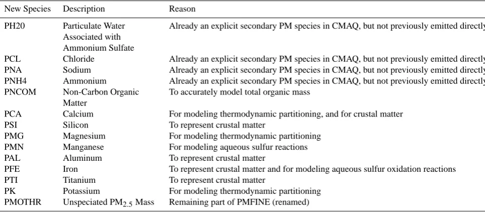
Finally, the speciation of PM2.5 emissions from all sources, including the dust sources, was updated. These up-dates to the speciation of PM2.5were based on the work of Reff et al. (2009), in which an inventory for trace metals from PM2.5 was derived using EPA’s SPECIATE database (EPA, 2006; Simon et al., 2010). Eighty-four composite PM2.5 pro-files containing 37 trace elements were then created and mapped to all available source classification codes. In this work, we break down the miscellaneous component of PM2.5 (aka PMFINE) into 14 components for modeling in CMAQ. These 14 components are shown in Table 2. The new spe-ciation allows the emission inventory to be viewed in much more detail. For example, 89 % of the Si inventory in the un-adjusted 2002 NEI is dominated by six sources: agricultural tilling, unpaved road dust, external combustion boilers (from electric generating units), paved road dust, construction, and mining and quarrying.
2.3 Chemical boundary conditions
The chemical BCs for the CMAQ model simulation were provided by an annual 2006 GEOS-Chem (Bey et al., 2001) simulation. The GEOS-Chem simulation utilized the pre-patch version 9-01-01 of the model with secondary organic aerosols enabled, and was run using 2.0◦×2.5◦ (latitude– longitude) horizontal grid spacing and 24 vertical layers.
The simulation utilized GOES-5 meteorology and the default emissions based on the 2005 EPA NEI.
Since GEOS-Chem and CMAQ use different names and definitions for a number of species, it is necessary to map the GEOS-Chem species to the CMAQ species. GEOS-Chem uses the Dust Entrainment and Deposition (DEAD) scheme with GOCART source function (Zender et al., 2003; Ginoux et al., 2001; Fairlie et al., 2007) and transports WBD in four size bins with edges at 0.1, 1, 1.8, 3.0, and 6 µm radii. For use in BCs, the GEOS-Chem dust was speciated into trace metals as well as other lumped species based on a composite of four desert soil profiles from SPECIATE, with eight pro-files (four for PM2.5and four for PM10)of desert soil used to create a composite profile based on the median value for each species. Dust from GEOS-Chem (DST1-4) is mapped to CMAQ species by first matching the GEOS-Chem size bins to the CMAQ modes. Dust in the smallest GEOS-Chem size-bin (DST1) was matched to the CMAQ accumulation mode species (J mode), while the three larger GEOS-Chem size bins (DST2-4) correspond to CMAQ’s coarse mode (K mode). GEOS-Chem dust is speciated according to a com-posite (mean) profile. Table 3 provides a complete mapping of the CMAQ inorganic species to the GEOS-Chem tracer species.
2.4 CMAQ model configuration
The CMAQ model simulation utilized the latest version of the model (v5.0) available for download from the Commu-nity Modeling and Analysis System (CMAS) Center web-site (http://www.cmascenter.org/). The CMAQv5.0 model in-cludes a number of improvements over the previous version of the model (v4.7.1), including an in-line photolysis cal-culation instead of look-up tables, a new condensed toluene mechanism for CB05 with chlorine chemistry (CB05TUCL), updated aerosol chemistry and speciation to include the de-tailed speciation profiles described in Sect. 2.2.2, a represen-tation of contributions from WBD, inclusion of NO emis-sions from lightning, an updated turbulent mixing scheme under stable conditions and an improved vertical advection scheme, as well as a number of additional updates to the model code structure. For additional details regarding the new features and enhancements in CMAQv5.0, the reader is referred to the release notes available for download along with the CMAQ model code.
Table 2. The revised speciation of PMFINE and the reasons for making them explicit.
New Species Description Reason
PH20 Particulate Water Associated with Ammonium Sulfate
Already an explicit secondary PM species in CMAQ, but not previously emitted directly
PCL Chloride Already an explicit secondary PM species in CMAQ, but not previously emitted directly PNA Sodium Already an explicit secondary PM species in CMAQ, but not previously emitted directly PNH4 Ammonium Already an explicit secondary PM species in CMAQ, but not previously emitted directly PNCOM Non-Carbon Organic
Matter
To accurately model total organic mass
PCA Calcium For modeling thermodynamic partitioning, and for crustal matter
PSI Silicon To represent crustal matter
PMG Magnesium For modeling thermodynamic partitioning PMN Manganese For modeling aqueous sulfur reactions
PAL Aluminum To represent crustal matter
PFE Iron To represent crustal matter and for modeling aqueous sulfur oxidation reactions
PTI Titanium To represent crustal matter
PK Potassium For modeling thermodynamic partitioning PMOTHR Unspeciated PM2.5Mass Remaining part of PMFINE (renamed)
The two most important changes in the new version of the model that affect the estimates of dust are the updates to the aerosol chemistry and speciation, and the representation of the effects of WBD in the model. In addition, changes to tur-bulent mixing and vertical advection also affect how dust is dispersed and transported in the model.
Enhancements to the aerosol module in CMAQv5.0 were directed both at improving the aerosol chemistry as well as speciation. Evaluation studies have revealed that the largest biases in CMAQ PM2.5results are driven by over predictions of the unspeciated PM2.5, referred to hereafter as PMother (Appel et al., 2008); this component constitutes over half of the NEI for PM2.5 using the old five-component chemical speciation scheme. Detailed speciation profiles derived from the work of Reff et al. (2009) were used to further subdi-vide emissions of PMother into primary ammonium (NH+4), sodium (Na+), chloride (Cl−), selected trace metals (Mg, Al, Si, K, Ca, Ti, Mn, and Fe), and non-carbon organic mass (NCOM).
The CMAQ transport and chemistry operators were fur-ther modified to explicitly represent these nine additional PM constituents. This additional speciation now allows for de-tailed characterization of the species, processes, and emis-sion sector contributions to the model bias in primary and consequently total PM. The explicit treatment of Fe and Mn also allows for explicit representation of their catalysis ef-fects on S(IV) to S(VI) conversion through aqueous chem-istry, and consequently more consistent treatment of sulfate (SO2−4 )production pathways in the model.
The representation of gas/particle partitioning of chlo-ride, ammonia, and nitrate was also improved through the incorporation of ISORROPIA version II (ISORROPIA II; Fountoukis and Nenes, 2007; Nenes et al., 1998, 1999).
In addition to more robust solutions compared to previ-ous versions of ISORROPIA, ISORROPIA II includes cal-cium (Ca2+), potassium (K+), and magnesium (Mg2+)ions, species abundant in sea salt and soil dust, which can affect the partitioning of semivolatile inorganic species. The ex-plicit representation of dust emission and PM composition simulated by CMAQv5.0 facilitates the expanded speciation and incorporation of ISORROPIA II.
Table 3. GEOS-Chem to CMAQ boundary condition mapping for dust and inorganic aerosol species. SALA and SALC represent accumu-lation and coarse sea salt in GEOS-Chem. SO4s and NITs are sulfate and nitrate formed on sea-salt aerosol. OCPI and OCPO are primary organic carbon in GEOS-Chem.
CMAQ Species GEOS-Chem Tracer
Coarse-mode aerosol
ASO4K 0.0776×SALC+0.02655×(DST2+DST3+DST4)+SO4s
ANO3K NITs+0.0016×(DST2+DST3+DST4)
ACLK 0.5538×SALC+0.01190×(DST2+DST3+DST4)
ASOIL 0.95995×(DST2+DST3+DST4)
Accumulation-mode aerosol
ASO4J 0.99×SO4+0.0776×SALA+0.0225×(DST1)
ANO3J 0.99×NIT+0.00020×(DST1)
ACLJ 0.5538×SALA+0.00945×(DST1)
ANH4J 0.99×NH4+0.00005×(DST1)
ANAJ 0.3086×SALA+0.03935×(DST1)
ACAJ 0.0118×SALA+0.07940×(DST1)
AKJ 0.0114×SALA+0.03770×(DST1)
APOCJ 0.999×(OCPI+OCPO)+0.01075×(DST1)
APNCOMJ 0.4×0.999×(OCPI+OCPO)+0.0043×(DST1)
AFEJ 0.03355×(DST1)
AALJ 0.05695×(DST1)
ASIJ 0.19435×(DST1)
ATIJ 0.0028×(DST1)
AMNJ 0.00115×(DST1)
AOTHRJ 0.50219×(DST1)
AMGJ 0.0368×SALA
Aitken-mode aerosol
ASO4I 0.01×SO4
ANO3I 0.01×NIT
ANH4I 0.01×NH4
APOCI 0.001×(OCPI+OCPO)
APNCOMI 0.4×0.001×(OCPI+OCPO)
3 Observation data
There are several sources of routine, ground-based observa-tions of PM that include observaobserva-tions of the speciated dust components. Both the Interagency Monitoring of Protected Visual Environments (IMPROVE; http://vista.cira.colostate. edu/improve/) and Chemical Speciation (CSN; http://www. epa.gov/ttnamti1/speciepg.html) networks provide surface measurements of total PM2.5 and PM10, along with speci-ated PM2.5measurements of SO2−4 , NO−3, NH+4, Na+, Cl−, and the trace metals of Mg, Al, Si, K, Ca, Ti, Mn, and Fe. The IMPROVE network consisted of 161 sites in 2006, with the majority of the sites located in the western United States. The IMPROVE network sites are typically located in rural areas, with a large number of the sites located in national parks, and as such the measurements tend to represent the background concentration of pollutants. Conversely, the CSN network consisted of 214 sites in 2006, primarily located in urban areas, with a larger majority of the sites located in the
eastern United States. In addition to data from the IMPROVE and CSN networks, the Clean Air Status and Trends Network (CASTNET) provides weekly average measurements of par-ticulate SO2−4 , NO−3, NH+4, and HNO3, along with gaseous SO2. There were 85 active CASTNET sites in 2006.
Soil is not directly measured at the IMPROVE and CSN sites but instead is derived from measurements of the var-ious trace metals at each monitoring site (Eq. 1). The soil equation is a useful aggregate measure of soil (as it could be tedious to examine each individual element separately). This equation was first developed by Malm et al. (1994), and accounts for mass associated with oxidized forms of aluminum, silicon, calcium, iron, and titanium. In addi-tion, the multiplication factors for each of these elements accounts for additional mass associated with soil organic matter, potassium, and other compounds. This soil equa-tion has been used to calculate soil contribuequa-tions to visi-bility degradation for the purpose of complying with the US EPA’s regional haze rule at IMPROVE monitoring lo-cations (http://vista.cira.colostate.edu/improve/publilo-cations/ graylit/023 SoilEquation/Soil Eq Evaluation.pdf). In this work, we define soil by applying Eq. (1) to measured data from IMPROVE and CSN networks, as well as to the CMAQ model data.
Soil=(2.20×Al)+(2.49×Si)+(1.63×Ca)+
(2.42×Fe)+(1.94×Ti) (1) The measurements of soil from both IMPROVE and CSN are for the fine (PM2.5) fraction of PM only. Any difference in comparing these measurements to the sum of the Aitken (i) and accumulation (j) modes from CMAQ is likely to be small overall, but could be more substantial in some in-stances.
A recent study by Indresand and Dillner (2012) showed that Si and Al measurements from the IMPROVE network are misreported when the sulfur to iron (S / Fe) ratio is large. This is due to low-energy spectral interference by S in the X-ray fluorescence spectrometry (XRF) instrument used for the IMPROVE sites. They examined IMPROVE data from 2008 and found that when the observed S / Fe ratio was less than 8, which constituted 49 % of the data, the reported Si and Al value were not affected by the S interference. For S / Fe ratios greater than 8 but less than 70 (47 % of the data), the Si value was overreported by up to 100 % and the Al value was either overreported by 50 % or incorrectly reported as below detection limit. For S / Fe ratios greater than 70 (4 % of the data), the Si value was overreported by a factor of 2 or more, while the Al value was misreported by±50 % or more. They advise using the IMPROVE Si and Al data cautiously when the S / Fe ratio is large (while those data are included in the analysis here, no strong conclusions are made based on those particular data). The CSN measurements do not suffer from the same issue as the IMPROVE measurements due to lower measured S concentrations (due to a lower flow rate) and better peak baseline separation between S, Si, and Al.
In addition to the potential issue with Al and Si measure-ments from the IMPROVE network, a separate analysis per-formed comparing soil measurements from IMPROVE and CSN sites revealed relative biases of up to 30 % or more in
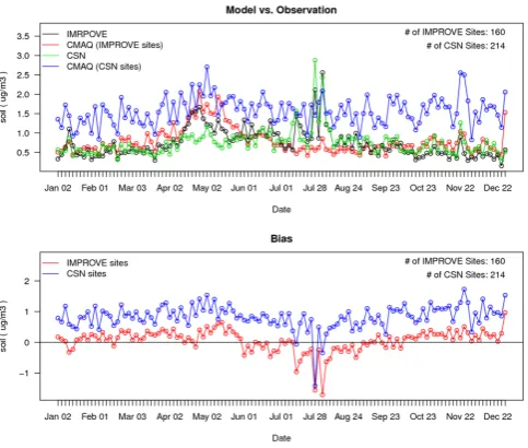
Fig. 1. The top time series plot shows the IMPROVE fine particu-late soil observations (black) versus CMAQ estimated soil (red) and CSN soil observations (green) versus CMAQ estimated soil (blue) for 2006 for all CONUS sites. The bottom time series plot shows the CMAQ bias for soil at the IMPROVE network sites (red) and CSN sites (blue). Both plots are in units of µg m−3.
the IMPROVE measurements, with higher IMPROVE con-centrations (Hand et al, 2011). Furthermore, analyses of IM-PROVE data suggest that PM2.5 soil mass concentrations may be underestimated by up to 20 % and have some regional dependence (Malm and Hand, 2007). Finally, Solomon et al. (2004) found that IMPROVE measurements of Fe, Si, and Ca were biased slightly high compared to STN (CSN) mea-surements, an issue they contribute to potential difference in inlet cut-point efficiencies.
4 CMAQ base model performance
4.1 Soil
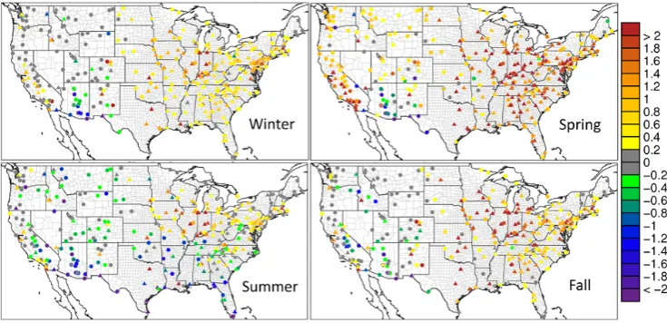
Fig. 2. Fine particulate soil seasonal mean bias (µg m−3) at the IMPROVE (circles) and CSN (triangles) network sites for the base CMAQ model simulation.
The CMAQ-model-estimated soil concentrations are in relatively good agreement with the IMPROVE network ob-servations throughout the year, with a mean bias generally less than±0.5 µg m−3, with the exception of several episodes in the summer. For the CSN sites, the model systematically overestimates the soil concentrations throughout the year, again with the exception of several episodes in the summer when soil is underestimated. These results are generally con-sistent with the results presented by Tong et al. (2012) for a 2002 CMAQ model simulation, which reported mean biases of 0.3 µg m−3and 1.2 µg m−3for January and−1.0 µg m−3 and−0.6 µg m−3for July for the IMPROVE and CSN net-works, respectively.
Figure 2 presents a spatial plot of seasonal mean bias for soil for the IMPROVE and CSN sites. In the winter (December–February), the model shows a large difference in bias between the eastern and western United States, with sites in the eastern United States (east of the Rocky Moun-tains) showing a moderate to large overestimation (positive bias) in soil and sites in the western United States show-ing generally unbiased to slightly underestimated (negative bias) soil concentrations (exception being central California, where soil concentrations are overestimated). In the spring (March–May), soil is overestimated by the model at the vast majority of the IMPROVE and CSN network sites. Only sites in the southwest United States (i.e., Utah, Colorado, Arizona, and New Mexico) show unbiased to slightly underestimated soil concentrations. In the summer (June–August), the bias trend is reversed, with the majority of sites showing a slight to moderate (1 µg m−3or less) underestimation of soil, the exception being in the Great Lakes region and small parts of the Northeast, where soil concentrations are still overes-timated. In the fall (September–November), the bias pattern is very similar to the winter, with soil concentrations overes-timated in the eastern United States and unbiased to slightly
underestimated in the western United States. Similar spatial trends for the summer and winter were reported by Tong et al. (2012).
Overall, soil is consistently overestimated in the east-ern United States throughout the year, while in the west-ern United States, soil estimates tend to fluctuate between a slight underestimation to slight overestimation. Airborne soil in the eastern United States is primarily the result of an-thropogenic sources, with a smaller contribution from natural WBD, whereas the western United States has a greater con-tribution to soil from WBD and long-range transport. Several possible reasons for the overestimation of dust in the eastern United States include AFD emissions that are too high in the model, an urban transportable fraction of dust that may be too large or too small, a contribution to soil from WBD that may be overestimated (should be small for eastern United States), and that the modeled PBL height in urban areas may be too low due to insufficient heat retention in urban areas (i.e., urban heat island effect). Several of these issues will be discussed further in Sect. 5. Additionally, the underestima-tion of soil in several areas for some time periods may be at least partially due to the wind-speed requirement in the cur-rent WBD implementation being too high, an issue that will be addressed in a future release of the model.
4.2 Trace metals
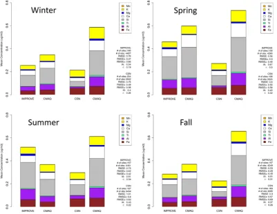
Fig. 3. Seasonal stacked bar plots of the observed concentrations (µg m−3) of the fine particulate trace metals Fe, Al, Ti, Si, Ca, Mg, K, and Mn for the IMPROVE and CSN networks and the corresponding model-estimated concentrations. Shown below the legend on each plot are root-mean-square error (RMSE), index of agreement (IA), and correlation coefficient (r) for each network.
is overestimated by∼40 % for IMPROVE and∼170 % for CSN. For the IMPROVE network, Fe, Al, Si, Ca, K, and Mn are overestimated by 20 % to 60 %, while Ti is overestimated by 90 % (the concentrations of Ti are very low however) and Mg is underestimated by 7 %. For the CSN, all the metals, with the exception of Mg, are overestimated by at least 70 %, with Al, Ti, Si, and Ca all overestimated by∼200 % or more. In the spring, the model performance is very similar to the winter, with the total concentration of all the trace metals overestimated by 30 % for the IMPROVE network and 170 % for the CSN. The performance of the individual trace metals is also similar, with most metals overestimated by 10 to 60 % (Mg is underestimated by 50 %) for the IMPROVE network. The model continues to significantly overestimate Al, Ti, Si, and Ca by 200 % or more at the CSN sites (Fe, Mg, K, and Mn are overestimated by 30 to 80 %).
In the summer, the total concentration of all the trace met-als is underestimated by 30 % for IMPROVE, but still over-estimated by 50 % for CSN. The largest underestimations for the IMPROVE network are in Fe (23 %), Al (47 %), Si (37 %), and Mg (61 %), while Ti, Ca, K, and Mn are all within 15 % of the observed concentration. For the CSN, the largest overestimations are in Al (220 %), Ti (297 %),
Si (165 %), Ca (145 %), and Mg (92 %), with smaller over-estimations in K (32 %) and Mn (48 %), while Fe is within 10 % of the observed concentration. In the fall, the total con-centration of all the trace metals is again overestimated for both the IMPROVE (30 %) and CSN (190 %) networks. The overestimations at IMPROVE sites in fall are very similar to the winter, with the largest overestimations in Ti (83 %), K (59 %), and Mn (42 %), smaller overestimations in Fe (16 %), Al (27 %), Si (28 %), and Ca (27 %), and an underestimation in Mg (10 %). For the CSN, the largest overestimations are in Al (380 %), Ti (370 %), Si (470 %), and Ca (206 %), with smaller overestimations in Fe (28 %), Mg (62 %), K (84 %), and Mn (16 %). Time series plots for the individual trace met-als can be found in the Supplement.
Fig. 4. Boxplots of observed (solid black; light shading) and CMAQ estimated (dashed red; dark shading) average diurnal concentrations (µg m−3) of Mn (left) and Ca (right) for Dearborn, Michigan, for 13 July–11 August 2007. The lines represent the median, while the shading represents the 25th to 75th (interquartile) range of the data.
trace metals). Similar overestimations have been observed in other primary emitted species (e.g., NO and CO) in urban areas. This is due to the tendency of the WRF model to un-derestimate the overnight mixing in urban areas (Makar et al., 2006), possibly due to PBL heights that are too low or a minimum eddy diffusivity (Kzmin)that is too small, which results in an overconcentration of pollutants near the surface, ultimately leading to high model biases. A number of the trace metals are emitted in urban areas from industrial op-erations that are continuous throughout the day and night. As such, those elements would tend to be overestimated during the night due to the insufficient mixing in the model. Work is currently underway to improve the nighttime mixing in ur-ban areas by adding impervious surface information (e.g., pavement) into the WRF model in order to capture the heat retention in cities, which ultimately would improve the rep-resentation of mixing during stable conditions in these urban environments.
4.3 Effect on sulfate chemistry
In previous versions of the CMAQ model, aqueous-phase SO2−4 production via the metal catalysis oxidation pathway was calculated using prescribed constant background con-centrations of 0.01 µg m−3for Fe(III) and 0.005 µg m−3 for Mn(II). As CMAQv5.0 contains predicted values of Fe and Mn, these tracked concentrations are now used to estimate the Fe(III) and Mn(II) values for the metal catalyzed oxi-dation pathway. In addition to using model-estimated values of Fe and Mn, the rate constant for in-cloud SO2 oxidation via metal catalysis was also updated in CMAQv5.0 follow-ing Martin and Good (1991). Previous versions of the model use the rate constant suggested by Walcek and Taylor (1986).
Alexander et al. (2009) implemented the reaction into a global chemical transport model and examined global impli-cations of the sulfur budget. Sarwar et al. (2013) followed the procedures of Alexander et al. (2009) and implemented it into the CMAQ model. The new rate constant was developed at a pH of 3.0. Similar to Alexander et al. (2009), the new rate constant in CMAQv5.0 is used for all pH. Additional details regarding the implementation of the new treatment of crustal elements in the sulfate chemistry in CMAQ can be found in Sarwar et al. (2013).
Figure 5 presents spatial plots of the difference in monthly average particulate SO2−4 between the CMAQv5.0 model simulation with the new crustal treatment and a simulation with the old treatment for January 2006. The SO2−4 concen-trations in January are much lower in the eastern US (where SO2−4 concentrations are typically the highest) in the simula-tion with the new crustal treatment than in the one with the old treatment (Fig. 5a). The change in model performance for SO2−4 in January as a result of the new crustal treat-ment is generally mixed, with some areas (e.g., southeast United States) showing a slight (<1 µg m−3)improvement in bias, while other areas (e.g., Great Lakes region) showing a slight increase in bias (Fig. 5b). In June (and summer in general), the difference in SO2−4 concentrations is relatively small compared to January, with a mixture of very small in-creases and dein-creases in SO2−4 concentrations over relatively small areas, and the change in SO2−4 performance (bias) is minimal.
Fig. 5. (a) Difference in January monthly average SO42− concen-trations (µg m−3) for the CMAQv5.0 base simulation and a CMAQ simulation with prescribed Fe and Mn values and the old rate con-stant. (b) Change in bias between the two CMAQ simulations at IM-PROVE (circles), CSN (triangles), and CASTNET (squares) sites. Warm colors indicate an increase in bias in the base simulation, while cool colors indicate a decrease in bias.
predicted Fe and Mn concentrations and then applies sol-ubility and oxidation state to calculate Fe(III) and Mn(II). In January, mean Fe(III) concentrations range from 0 to 0.07 µg m−3 and mean Mn(II) concentrations range from 0 to 0.06 µgm−3in the eastern US. However, the domain-wide monthly mean Fe(III) concentration in the same region is 0.003 µg m−3, which is three times lower than the prescribed constant value used in previous versions of the model. Sim-ilarly, the domain-wide monthly mean Mn(II) concentration is 0.0008 µg m−3, which is six times lower than the constant prescribed value used in the previous versions of the model.
The new rate constant can be higher or lower than the old rate constant, depending on the pH. The impact of these changes on model-estimated SO2−4 concentrations is small in the summer, as expected, since SO2−4 production is pre-dominantly due to oxidation by H2O2 and OH. In winter, when the levels of these oxidants are lower, the contribu-tion of the aqueous Fe/Mn catalysis reaccontribu-tion pathway be-comes important. As a result, the change from the old crustal
Fig. 6. Observed (top) and CMAQ simulated (bottom) average fine particulate soil concentrations (µg m−3) as estimated by the PROVE soil equation for 13 July, 28 July, and 4 August 2006. IM-PROVE sites are indicated by circles; CSN sites are indicated by triangles.
treatment in CMAQv4.7 to the new treatment in CMAQv5.0 has the greatest impact on SO2−4 concentrations in the win-ter. It should also be noted that the relatively good agreement between CMAQ and observed concentrations (Fig. 3) builds confidence in the ability to integrate these model-estimated concentrations into the CMAQ chemistry.
4.4 Impact on soil concentrations from African dust events
to the average mean observed soil concentration for July and August (not shown), which is typically less than 4 µg m−3for the same region.
One possible cause of the high observed soil concentra-tions in July and August could be transported dust from the African continent, particularly from the Sahara region (Perry et al., 1997; Bates et al., 2008). In the summer, westerly flow in the subtropical region of the Northern Hemisphere can transport dust from the Sahara west across the Atlantic Ocean, sometimes reaching as far west as the CONUS. As these events are influence by dust from outside the CMAQ model domain, they need to be captured in the input BCs from GEOS-Chem. The GEOS-Chem model has demon-strated the ability to simulate the long-range transport of Sa-haran dust (Fairlie et al., 2007). Furthermore, an analysis aerosol optical depth (AOD) from satellite imagery, indica-tive of a dense concentration of particles in the troposphere, for late July and early August 2006 showed relatively high AOD values extending from Africa across the subtropical At-lantic Ocean to the east coast of the United States.
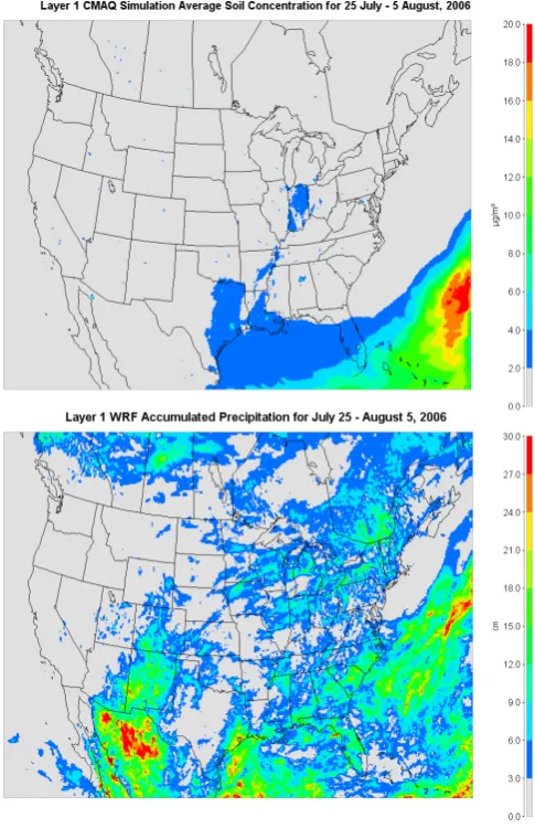
Figure 7 shows the average surface-level soil concentra-tion from 25 July through 5 August 2006, which covers two of the three high soil concentration episodes in the eastern United States identified from Fig. 1. For the 12-day period, the GEOS-Chem-derived BCs capture high concentrations of soil (up to 20 µg m−3)along the southeastern boundary of the CMAQ model domain, which spread westward toward the CONUS. However, while the BC inputs include elevated soil concentrations, the high concentrations of soil do not progress far enough west to reach the eastern United States, with most of the soil being removed before it makes it to the coastal and inland areas (although some relatively high soil concentrations are observed in Florida).
One possible reason the high soil concentrations are not estimated correctly for the interior eastern United States may be due to an overestimation of convection and precipitation by the WRF model off the southeast coast of the United States and along the Gulf Stream, which results in exces-sive removal of dust by wet deposition. Figure 7 presents the WRF accumulated precipitation for the period of 25 July through 5 August 2006. The WRF model estimates for pre-cipitation are large off the east coast of the United States, as well as in parts of the Caribbean, over Florida, and in the Gulf of Mexico. Unfortunately, little data exist with which to verify the precipitation estimates over the water (although some satellite-derived precipitation data are available, they were not examined here). However, Park et al. (2006) and Fairlie et al. (2007) note a similar underestimation of dust concentrations in Florida by the GEOS-Chem model due to excessive wet deposition (also the result of an overestimation of convective precipitation by the meteorological model).
Another reason for the lack of westward transport of the dust from the boundary may be due to incorrect wind flow or wind flow that is too weak off the southeast coast and in the Gulf of Mexico, which would result in the dust being
Fig. 7. Layer 1 CMAQ average soil concentration (top; µg m−3) and WRF accumulated total precipitation (bottom; cm) for 25 July– 5 August 2006.
advected in the wrong direction or settling out into the ocean before it reaches land. Additional sensitivity analyses with the WRF simulation are needed to confirm this as a possible cause of the transported dust issue within the CMAQ model simulation.
5 CMAQ model sensitivities
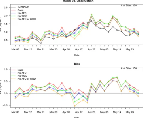
Fig. 8. Time series of IMPROVE-network-observed (black) and CMAQ-simulated soil concentrations (µg m−3; top) for the spring with the base CMAQ model simulation shown in red, the simula-tion with AFD emissions removed shown in blue, the simulasimula-tion with WBD effects removed shown in green, and the simulation with both AFD emissions and the effects of WBD removed shown in or-ange. The bottom time series shows the corresponding mean bias (µg m−3) for the same model simulations.
simulation for the same time period, and the impact of each change on the model estimates is assessed.
5.1 Effect of AFD emissions updates
Figures 8 and 9 present time series of observed soil concen-trations from the IMPROVE and CSN networks, respectively, and the corresponding model simulated soil concentrations for several CMAQ model sensitivities for the spring period. As noted previously in Fig. 1, the base CMAQ model simu-lation soil concentrations are slightly overestimated for most of the period compared to the observed soil concentrations from the IMPROVE network, with the largest overestima-tions from late April to late May. However, for the CSN, soil concentrations are typically overestimated by 1 µg m−3 or more for the entire period in the base simulation. The largest source of soil (trace metals) emissions in the emissions in-ventory (based on total soil emissions) is AFD (75 %), fol-lowed by electric generation units (EGUs; 13 %), industrial mineral processes (2 %), industrial fuel consumption (2 %), and industrial metal production (2 %).
Figure 10 (top panel) shows the change in soil absolute bias as a result of removing the AFD emissions, with warm colors indicating the bias increased in the simulation with no AFD emissions, while cool colors indicate the bias decreased in the simulation with no AFD emissions. The seasonal av-erage bias in soil decreases by between 0.1 and 0.7 µg m−3 in the eastern United States as a result of removing the AFD
Fig. 9. Time series of CSN observed (black) and CMAQ simu-lated soil concentrations (µg m−3; top) for the spring with the base CMAQ model simulation shown in red, the simulation with AFD emissions removed shown in blue, the simulation with WBD ef-fects removed shown in green, and the simulation with both AFD emissions and the effects of WBD removed shown in orange. The bottom time series shows the corresponding mean bias (µg m−3) for the same model simulations.
emissions, with the largest decrease in bias in the upper Mid-west and Great Lakes regions. The bias increases slightly (between 0.1 and 0.5 µg m−3) in the southwestern United States in the simulation with AFD emissions removed, in-cluding increases in bias at sites in Texas and Oklahoma. Overall, removing the AFD emissions results in a large re-duction in the soil bias in the eastern United States in the spring, suggesting there is an overestimation of the AFD emissions as well as likely issues with their diurnal temporal allocation.
5.2 Effect of WBD mechanism
The CMAQ model estimates for the simulation in which the effects of WBD were removed (NoWBD) are lower than the base-model-simulated soil concentrations but not as low as the simulation where AFD emissions were removed. The largest decrease in soil concentrations in the NoWBD sim-ulation compared to the base simsim-ulation occur in the late March through mid-April period (Figs. 8 and 9), indicating the effects of WBD in the model are significant during that period. Conversely, there is very little difference between the base simulation and the NoWBD simulation from mid-April through the end of May, suggesting the WBD effects are small.
Fig. 10. Difference in average soil concentration bias (µg m−3) for spring (2006) between the CMAQ simulation with no AFD emis-sions and the base CMAQ simulation (No AFD – Base; top), the CMAQ simulation with no WBD and the base CMAQ simulation (No WBD – Base; middle), and the CMAQ simulation with no WBD or AFD emissions and the base CMAQ simulation (No AFD or WBD – Base; bottom). Circles indicate IMPROVE network sites and triangles indicate CSN sites.
largest impact on the model simulated soil concentrations oc-curs in the arid/semi-arid regions of the southwestern United States, with the bias slightly higher in the NoWBD simula-tion versus the base simulasimula-tion. There is little to no impact to the bias in the eastern United States, where the bias in soil was highest in the base simulation (Fig. 2). These results suggest that an overestimation of WBD is not responsible for the high model-estimated soil concentrations in the eastern United States in the spring, where the effects of WBD should be small anyway.
5.3 Effect of both AFD and WBD
The final sensitivity performed removes the effects of both WBD and AFD emissions (referred to simply as NoDust) in order to assess the cumulative impact that those two up-dates to modeling system had on the model estimates of soil. The NoDust model simulation always has lower soil
concentrations than the base simulation and the NoWBD simulation (Figs. 8 and 9). There are several days dur-ing which the effects of either the AFD emissions (e.g., 24 March) or WBD (e.g., 2 April) dominate the change in soil concentrations compared to the base simulation. In ad-dition, soil concentrations are underestimated during the pe-riods from 3 March to 12 March and 14 April to 23 April in the NoDust simulation, which are the only periods when soil is underestimated at the IMPROVE network sites (Fig. 8).
It is clear from the plots in Fig. 10 that the change in bias in the NoDust simulation is dominated by the removal of the AFD emissions, with the effect of removing WBD limited in time and space. Since AFD emissions and WBD should be nonzero, the result of improved model performance when those emissions are removed entirely suggests that there are other errors in the modeling system (e.g., emission inputs) that contribute to an overestimation of soil. Wind-blown dust generally constitutes a small, temporally and spatially local-ized contribution to the soil concentrations in the model, with the largest contribution to soil limited primarily to the spring period in the desert southwest of the United States (although small effects are seen throughout the year). The systematic overestimation of soil across most of the domain throughout the year, even when the AFD emissions are removed, sug-gests that other emissions of the trace elements in the soil equation are overestimated.
6 Summary
Mineral dust, or soil, can constitute a significant portion of observed airborne PM in the United States, especially in eas where agriculture and construction are prevalent, or in ar-eas where WBD is common (e.g., southwest United States). The latest release of the CMAQ modeling system includes updated AFD emissions from agricultural farming and con-struction and the effects of WBD. To assess the CMAQ model estimates of soil and trace metals, an annual model simulation for the year 2006 was performed for the CONUS using the updated emissions inventory with AFD emissions and the effects of WBD included. The results of the model simulation were compared against ground-based observa-tions of soil and trace metals from the IMPROVE and CSN networks.
overestimated, including very large overestimations of Al, Ti, and Si in the fall. The underestimation of nighttime mixing in the urban areas, where most of the CSN sites are located, contributes to the overestimation of predicted trace metal concentrations. Work is currently underway to improve the representation of mixing during stable conditions in urban areas by including the heat retention due to impervious sur-faces (e.g., pavement) in the WRF model.
While the model typically overestimates soil concentra-tions, there are several localized episodes during the sum-mer, when soil concentrations are grossly underestimated by the model. Analysis suggests these observed elevated soil events are the result of long-range transport of dust from the African continent, and while the GEOS-Chem model simu-lation captures these events, the CMAQ modeling system has difficulty transporting the high soil concentrations from the boundary into the interior United States, which may be due to an overestimation of convective activity (e.g., precipita-tion) in the WRF model simulation that results in too much deposition. However, more analysis is needed to determine the exact cause of the underestimation of soil in the CMAQ model during these dust events.
In addition to the base model simulation, several model sensitivity simulations were also performed for the spring period to assess the impact of uncertainties in AFD emis-sions and natural WBD dust emission estimates on the model estimates of soil. As expected, removing the AFD emis-sions resulted in substantially lower model soil concentra-tions. Similarly, removing the effects of WBD emissions also lowered the model soil concentrations, but to a much lesser extent than removing the AFD emissions. Even with both AFD emissions and WBD effects removed, soil concentra-tions were still often overestimated, suggesting that there are other sources of errors in the modeling system that contribute to the overestimation of soil. In particular, other sources of trace elements in the emissions inventory are likely overesti-mated, such as emissions from EGUs or other industrial min-eral/metal production processes. Efforts are currently under-way to further improve the dust categories in the NEI, in-cluding possible adjustments to the seasonal and/or diurnal temporal profile of emissions.
Supplementary material related to this article is available online at: http://www.geosci-model-dev.net/6/ 883/2013/gmd-6-883-2013-supplement.pdf.
Acknowledgements. The authors would like to thank Lara Reynolds of Computer Sciences Corporation for performing the WRF model simulations used in this study. Thanks to Prakash Bhave for his contributions to this work, specifically for his help speciating PMotherinto the various trace elements and his many other sugges-tions along the way that contributed significantly to this project. Thanks also to Matt Landis and Gary Norris for providing and con-sulting on the continuous trace metal measurements from Dearborn.
Edited by: A. Lauer
Disclaimer. The United States Environmental Protection Agency through its Office of Research and Development supported the re-search described here. It has been subjected to Agency review and approved for publication.
References
Alexander, B., Park, R. J., Jacob, D. J., and Gong, S.: Transition metal-catalyzed oxidation of atmospheric sulfur: global impli-cations for the sulfur budget, J. Geophys. Res., 114, D02309, doi:10.1029/2008JD010486, 2009.
Allen, D. J., Pickering, K. E., Pinder, R. W., Henderson, B. H., Appel, K. W., and Prados, A.: Impact of lightning-NO on east-ern United States photochemistry during the summer of 2006 as determined using the CMAQ model, Atmos. Chem. Phys., 12, 1737–1758, doi:10.5194/acp-12-1737-2012, 2012.
Appel, K. W., Bhave, P. V., Gilliland, A. B., Sarwar, G., and Roselle, S. J.: Evaluation of the Community Multiscale Air Qual-ity (CMAQ) model version 4.5: Sensitivities impacting model performance; Part II – particulate matter, Atmos. Environ., 42, 6057–6066, 2008.
Appel, K. W., Gilliam, R. C., Davis, N., Zubrow, A., and Howard, S. C.: Overview of the Atmospheric Model Evaluation Tool (AMET) v1.1 for evaluating meteorological and air quality mod-els, Environ. Modell. Softw., 26, 434–443, 2011.
Bates, T. S., Quinn, P. K., Coffman, D., Schulz, K., Covert, D. S., Johnson, J. E., Williams, E. J., Lerner, B. M., Angevine, W. M., Tucker, S. C., Brewer, W. A., and Stohl, A.: Boundary layer aerosol chemistry during TexAQS/GoMACCS 2006: In-sights into aerosol sources and transformation processes, J. Geo-phys. Res., 113, D00F01, doi:10.1029/2008JD010023, 2008. Bey, I., Jacob, D. J., Yantosca, R. M., Logan, J. A., Field, B. D.,
Fiore, A. M., Li, Q., Liu, H. Y., Mickley, L. J., and Schultz, M. G.: Global modeling of tropospheric chemistry with assim-ilated meteorology: Model description and evaluation, J. Geo-phys. Res., 106, 23073–23096, 2001.
Byun, D. W. and Ching, J. K. S.: Science algorithms of the EPA models-3 Community Multiscale Air Quality (CMAQ) modeling system, EPA-600/R-99/030, 1999.
Byun, D. W. and Schere, K. L.: Review of the governing equations, computational algorithms, and other components of the models-3 Community Multiscale Air Quality (CMAQ) modeling system, Appl. Mech. Rev., 59, 51–77, 2006.
EPA: SPECIATE 4.0: Speciation database development doc-umentation final report, EPA/600/R-06/161, available at: http://www.epa.gov/ttn/chief/software/speciate/speciate4/ documentation/speciatedoc 1206.pdf (last access: 1 July 2013), 2006.
Etyemezian, V., Ahonen, S., Nikolic, D., Gillies, J., Kuhns, H., Gillette, D., and Veranth, J.: Deposition and removal of fugi-tive dust in the arid southwestern United States: measurements and model results, J. Air Waste Manage. Assoc., 54, 1099–1111, 2004.
Foley, K. M., Roselle, S. J., Appel, K. W., Bhave, P. V., Pleim, J. E., Otte, T. L., Mathur, R., Sarwar, G., Young, J. O., Gilliam, R. C., Nolte, C. G., Kelly, J. T., Gilliland, A. B., and Bash, J. O.: Incremental testing of the Community Multiscale Air Quality (CMAQ) modeling system version 4.7, Geosci. Model Dev., 3, 205–226, doi:10.5194/gmd-3-205-2010, 2010.
Fountoukis, C. and Nenes, A.: ISORROPIA II: a computa-tionally efficient thermodynamic equilibrium model for K+ -Ca2+-Mg2+-NH+4-Na+-SO2−4 -NO−3-Cl−-H2O aerosols, At-mos. Chem. Phys., 7, 4639–4659, doi:10.5194/acp-7-4639-2007, 2007.
Gilliam, R. C., Godowitch, J. M., and Rao, S. T.: Improving the horizontal transport in the lower tropospher with four di-mensional data assimilation, Atmos. Environ., 53, 186–201, doi:10.1016/j.atmosenv.2011.10.064, 2012.
Ginoux, P., Chin, M., Tegen, I., Prospero, J. M., Holben, B., Dubovik, O., and Lin, S. J.: Sources and distributions of dust aerosols simulated with the GOCART model, J. Geophys. Res., 106, 20255–20273, 2001.
Hand, J. L., Copeland, S. A., Day, D. E., Dillner, A. M. Indresand, H., Malm, W. C., McDade, C. E., Moore, C. T., Pitchford, M. L., Schichtel, B. A., and Watson, J. G.: Spatial and seasonal patterns and temporal variability of haze and its constituents in the United States, Report V, available at: http://vista.cira.colostate.edu/improve/Publications/ Reports/2011/PDF/IMPROVE V FullReport.pdf (last access: 1 July 2013), 2011.
Houyoux, M. R., Vukovich, J. M., Coats Jr., C. J., Wheeler, N. J. M., and Kasibhatla, P.: Emission inventory development and process-ing for the seasonal model for regional air quality, J. Geophys. Res., 105, 9079–9090, 2000.
Iacono, M. J., Delamere, J. S., Mlawer, E. J., Shephard, M. W., Clough, S. A., and Collins, W. D.: Radiative forcing by long-lived greenhouse gases: Calculations with the AER ra-diative transfer models, J. Geophys. Res., 113, D13, D13103, doi:10.1029/2008JD009944, 2008.
Indresand, H. and Dillner, A. M.: Experimental character-ization of sulfur interference in IMPROVE aluminum and silicon XRF data, Atmos. Environ., 61, 140–147, doi:10.1016/j.atmosenv.2012.06.079, 2012.
Kain, J. S.: The Kain-Fritsch convective parameterization: An up-date, J. Appl. Meteor., 43, 170–181, 2004.
Makar, P. A., Gravel, S., Chirkov, V., Strawbridge, K. B., Froude, F., Arnold, J., and Brook, J.: Heat flux, urban properties, and re-gional weather, Atmos. Environ., 40, 2750–2766, 2006. Malm, W. C. and Hand, J. L.: An examination of the physical and
optical properties of aerosols collected in the IMPROVE pro-gram, Atmos. Environ., 41, 3407–3427, 2007.
Malm, W. C., Sisler, J. F., Huffman, D., Eldred, R. A., and Cahill, T. A.: Spatial and seasonal trends in particle concentration and op-tical extinction in the United States, J. Geophys. Res., 99, 1347– 1370, 1994.
Martin, R. L. and Good, T. W.: Catalyzed oxidation of sulfur diox-ide in solution: the iron-manganese synergism, Atmos. Environ., 25A, 2395–2399, 1991.
Morrison, H., Thompson, G., and Tatarskii, V.: Impact of cloud mi-crophysics on the development of trailing stratiform precipitation in a simulated squall line: Comparison of one- and two-moment schemes, Mon. Weather Rev., 137, 991–1007, 2009.
Nenes, A., Pandis, S. N., and Pilinis, C.: ISORROPIA: A new ther-modynamic equilibrium model for multiphase multicomponent inorganic aerosols, Aquat. Geochem., 4, 123–152, 1998. Nenes, A., Pandis, S. N., and Pilinis, C.: Continued development
and testing of a new thermodynamic aerosol module for urban and regional air quality models, Atmos. Environ., 33, 1553– 1560, 1999.
Otte, T. L. and Pleim, J. E.: The Meteorology-Chemistry Inter-face Processor (MCIP) for the CMAQ modeling system: up-dates through MCIPv3.4.1, Geosci. Model Dev., 3, 243–256, doi:10.5194/gmd-3-243-2010, 2010.
Pace, T. G.: Methodology to Estimate the Transportable Frac-tion (TF) of Fugitive Dust Emissions for Regional and Ur-ban Scale Air Quality Analyses, US EPA, Research Trian-gle Park NC, available at: http://www.epa.gov/ttnchie1/emch/ dustfractions/transportable fraction 080305 rev.pdf (last access: 1 July 2013), 2005.
Pancras, J. P., Landis, M. S., Norris, G. A., Vedantham, R., and Dvonch, J. T.: Source apportionment of ambient fine particu-late matter in Dearborn, Michigan, using hourly resolved PM chemical composition data, Sci. Total Environ., 448, 2–13, doi:10.1016/j.scitotenv.2012.11.083, 2013.
Park, R. J., Jacob, D. J., Kumar, N., and Yantosca, R. M.: Regional visibility statistics in the United States: Natural and transbound-ary pollution influences, and implications for the Regional Haze Rule, Atmos. Environ., 40, 5405–5423, 2006.
Perry, K. D., Cahill, T. A., Eldred, R. A., Dutcher, D. D., and Gill, T. E.: Long-range transport of North African dust to the eastern United States, J. Geophys. Res., 102, 11225–11238, 1997. Pleim, J. E.: A combined local and nonlocal closure model for the
atmospheric boundary layer. Part I: model description and test-ing, J. Appl. Meteor. Clim., 46, 1383–1395, 2007a.
Pleim, J. E.: A combined local and nonlocal closure model for the atmospheric boundary layer. Part II: application and evaluation in a mesoscale meteorological model, J. Appl. Meteor. Clim., 46, 1396–1409, 2007b.
Pleim, J. E. and Xiu, A.: Development and testing of a surface flux and planetary boundary layer model for application in mesoscale models, J. Appl. Meteor., 34, 16–32, 1995.
Pouliot, G., Simon, H., Bhave, P., Tong, D., Mobley, D., Pace, T., and Pierce, T.: Assessing the anthropogenic fugitive dust emission inventory and temporal allocation using an updated speciation of particulate matter, International Emission Inven-tory Conference, San Antonio, TX, September 27–30, avail-able at: http://www.epa.gov/ttn/chief/conference/ei19/session9/ pouliot.pdf, 2010.
Reff, A., Bhave, P. V., Simon, H., Pace, T. G., Pouliot, G. A., Mob-ley, J. D., and Houyoux, M.: Emissions Inventory of PM2.5Trace Elements across the United States, Environ. Sci. Technol., 43, 5790–5796, 2009.
Sarwar, G., Fahey, K., Kwok, R., Roselle, S. J., Mathur, R., Xue, J., Yu, J., and Carter, W. P. L.: Potential impacts of two SO2 oxidation pathways on regional sulfate concentrations: aqueous-phase oxidation by NO2and gas-phase oxidation by Stabilized Criegee Intermediates, Atmos. Environ., 68, 186–197, 2013. Simon, H., Beck, L, Bhave, P. V., Divita, F., Hsu, F., Hus, Y.,
Skamarock, W. C., Klemp, J. B., Dudhia, J., Gill, D. O., Barker, D. M., Duda, M. G., Huang, X-Y, Wang, W., and Powers, J. G.: A description of the advanced research WRF version 3. NCAR Tech Note NCAR/TN 475 STR, 125 pp., available from UCAR Communications, P.O. Box 3000, Boulder, CO 80307, 2008. Sokolik, I. N. and Toon, O. B.: Direct radiative forcing by
anthro-pogenic airborne mineral aerosols, Nature, 381, 681–683, 1996. Solomon, P. A., Klamser-Williams, T., Egeghy, P. P., Crumpler, D., Rice, J., Ashbaugh, L., and McDade, C.: Multi-site comparison of mass and major chemical components obtained by collocated STN and IMPROVE chemical speciation network monitors, pre-sented at American Association for Aerosol Research 2004 An-nual Conference, Atlanta, GA, 4–8 October, 2004.
Swall, J. and Foley, K. M.: The impact of spatial correlation and incommensurability on model evaluation, Atmos. Environ., 43, 1204–1217, 2009.
Tong, D. Q., Dan, M., Wang, T., and Lee, P.: Long-term dust clima-tology in the western United States reconstructed from routine aerosol ground monitoring, Atmos. Chem. Phys., 12, 5189–5205, doi:10.5194/acp-12-5189-2012, 2012.
Veranth, J. M., Pardyjak, E. R., and Seshadri, G.: Vehicle-generated fugitive dust transport: analytic models and field study, Atmos. Environ., 37, 2295–2303, 2003.
Vukovich, J. and Pierce, T.: The Implementation of BEIS3 within the SMOKE Modeling Framework, In Proceedings of the 11th International Emissions Inventory Conference, Atlanta, Georgia, 15–18 April, available at: www.epa.gov/ttn/chief/conference/ ei11/modeling/vukovich.pdf, 2002.
Walcek, C. J. and Tyalor, G. R.: A theoretical method for comput-ing vertical distributions of acidity and sulfate production with cumulus clouds, J. Atmos. Sci., 43, 339–355, 1986.
Watson, J. G. and Chow, J. C.: Reconciling urban fugitive dust emissions inventory and ambient source contribution estimates: Summary of current knowledge and needed research, DRI docu-ment (6110.4), 240, available at: www.epa.gov/ttn/chief/efdocs/ fugitivedust.pdf, 2000.
Xiu, A. and Pleim, J. E.: Development of a land-surface model. Part I: application in a mesoscale meteorological model, J. Appl. Me-teor., 40, 192–209, 2001.
Yarwood, G., Roa, S., Yocke, M., and Whitten, G.: Updates to the carbon bond chemical mechanism: CBo5. Final report to the US EPA, RT-0400675, available at: http://www.camx.com, http: //www.camx.com/publ/pdfs/cb05 final report 120805.aspx (last access: 1 July 2013), 2005.