www.geosci-model-dev.net/2/113/2009/
© Author(s) 2009. This work is distributed under the Creative Commons Attribution 3.0 License.
Geoscientific
Model Development
LANL
∗
V1.0: a radiation belt drift shell model suitable for real-time
and reanalysis applications
J. Koller, G. D. Reeves, and R. H. W. Friedel
Space Science and Applications, ISR-1, Los Alamos National Lab, USA
Received: 8 December 2008 – Published in Geosci. Model Dev. Discuss.: 11 February 2009 Revised: 7 July 2009 – Accepted: 28 July 2009 – Published: 29 July 2009
Abstract. We describe here a new method for calculating the magnetic drift invariant, L∗, that is used for modeling radiation belt dynamics and for other space weather appli-cations. L∗ (pronounced L-star) is directly proportional to the integral of the magnetic flux contained within the sur-face defined by a charged particle moving in the Earth’s geo-magnetic field. Under adiabatic changes to the geogeo-magnetic fieldL∗is a conserved quantity, while under quasi-adiabatic fluctuations diffusion (with respect to a particle’sL∗) is the primary term in equations of particle dynamics. In particu-lar the equations of motion for the very energetic particles that populate the Earth’s radiation belts are most commonly expressed by diffusion in three dimensions: L∗, energy (or momentum), and pitch angle (the dot product of velocity and the magnetic field vector). Expressing dynamics in these co-ordinates reduces the dimensionality of the problem by ref-erencing the particle distribution functions to values at the magnetic equatorial point of a magnetic “drift shell” (or L-shell) irrespective of local time (or longitude). While the use ofL∗aids in simplifying the equations of motion, practical applications such as space weather forecasting using realistic geomagnetic fields require sophisticated magnetic field mod-els that, in turn, require computationally intensive numerical integration. Typically a singleL∗calculation can require on the order of 105 calls to a magnetic field model and each point in the simulation domain and each calculated pitch an-gle has a different value ofL∗. We describe here the devel-opment and validation of a neural network surrogate model for calculatingL∗in sophisticated geomagnetic field models with a high degree of fidelity at computational speeds that are millions of times faster than direct numerical field line
Correspondence to: J. Koller
mapping and integration. This new surrogate model has ap-plications to real-time radiation belt forecasting, analysis of data sets involving tens of satellite-years of observations, and other problems in space weather.
1 Introduction
the “Office National d’Etudes et Recherches A´erospatiales” (ONERA) and the Dynamic Radiation Environment Assim-ilation Model (DREAM) (Reeves et al., 2008) developed by Los Alamos National Laboratory (LANL).
The large scale motion of charged particles in the Earth’s magnetosphere are dominated by the structure of the global geomagnetic and geoelectric fields. At sufficiently high en-ergies (tens or hundreds of keV) the electric field can be ne-glected and particle motion can be described by three pe-riodic motions: gyration around the magnetic field, bounce along the magnetic field between magnetic mirror points, and gradient/curvature drift across the magnetic field in an az-imuthal direction around the Earth. Each periodic motion has a Hamiltonian invariant and in the Earth’s field they are well separated by the adiabatic time scales. The gyro-invariant is the magnetic moment,µ, which is invariant on millisecond time scales. The bounce invariant, given byK, is related to the magnetic field integrated along the field between mirror points and has time scales of seconds. The drift invariant,8, integrates the magnetic field along a bounce path and again azimuthally around the earth on a closed shell. If the mag-netic field changes slowly relative to a drift period (hours) then the drift path is closed and8is adiabatically conserved. A more convenient quantity isL∗ (L-star) which is defined as
L∗= −2π k0
8RE
, (1)
wherek0is the Earth’s dipole moment andRE is the radius of the Earth (6370 km) and8is defined as
8= Z
B·dS. (2)
In a dipole magnetic field,L∗is the distance from the center of the Earth to the equatorial point of a given field line, in units of Earth radii. All pitch angles have the sameL∗for a given point in space. See also, Roederer (1970); Schulz and Lanzerotti (1974); Schulz (1991). Geosynchronous orbit, for example is atL∗=6.6.
One important challenge for modeling of the radiation belts (and other populations in space) is that the charged par-ticles moving in space form complex current systems that in turn distort the geomagnetic field. The interaction of the so-lar wind, magnetospheric, and ionospheric current systems form an interconnected dynamic system that produces strong distortions of the Earth’s field such that it no longer approxi-mates a dipole and, indeed, requires sophisticated numerical field models that are themselves subject of intensive research. Many models of the Earth’s geomagnetic field have been developed but both the pace of development and the numeri-cal sophistication of the models has increased dramatinumeri-cally in the last several decades. Numerically simple models such as the static Olsen-Pfitzer model (Olson and Pfitzer, 1977) have given way to dynamic, statistical models driven by a host
of solar wind and geomagnetic inputs. The models devel-oped by Tsyganenko and colleagues are representative and are among the most widely used (Tsyganenko et al., 2003; Tsyganenko and Sitnov, 2005). At an even higher level of complexity are globally self-consistent physics based mod-els but these modmod-els are sufficiently computer-intensive that they are typically only used for analysis in limited and tar-geted studies (e.g. Zaharia et al., 2006).
The motion of particles in complex, realistic geomag-netic field configurations can be closely approximated us-ing “guidus-ing center” theory representus-ing motion as functions of the three adiabatic invariants, µ, K, and L∗. The first two invariants are relatively easy to calculate even in so-phisticated modern field models because they involve only the local field and a one-dimensional integral along a sin-gle field line. The third invariant L∗ is much more diffi-cult, and computationally expensive, to calculate because it is both two-dimensional and global (McCollough et al., 2008). Typical integration requires on the order of 105calls to the magnetic field model for obtaining the magnetic field vec-tor. The resulting long computation times often pushes re-searchers to compromise and use simpler, less accurate mag-netic field models which may produce large inaccuracies and even wrong conclusions.
Huang et al. (2008) recently quantified the effect of us-ing various magnetic field models for radiation belt studies for calculatingL∗and other quantities in the radiation belts. They found that during storm timesL∗can vary by as much as 50% (C.-L. Huang, personal communication, 2008) be-tween the different models. As part of the DREAM project, Chen et al. (2007) studied the effect of using different mag-netic field models on the phase space density calculation and also found that an accurate magnetic field model is critical to accurate radiation belt modeling.
Further development of radiation belt and space weather models requires techniques that are computationally feasible and still use the most accurate magnetic field models avail-able. Direct numerical integration of the magnetic field can use certain well-known techniques and/or the brute force of many processors but other approaches that do not sacrifice accuracy for speed are also possible.
In this paper, we present a new method of calculating
L∗ using a neural network based surrogate model to repro-duce the same quantity calculated by direct numerical in-tegration of the so-called Tsyganenko-03, or TSK03 model (also known as the T01-storm inside the original source code) (Tsyganenko, 2002a,b; Tsyganenko et al., 2003). We note however, that the method applies equally to any mag-netic field model of arbitrary complexity – statistical, em-pirical, physics-based (e.g. magneto-hydrodynamic models), etc. We refer to this numerical application as the Los Alamos National LaboratoryL∗model, or LANL∗for short.
used here to illustrate the technique and Sect. 5 discusses how the network was trained. We validated and tested the neural network as explained in Sect. 6. We summarize and conclude with Sect. 7.
2 Surrogate models
Surrogate models (meta-models, or response surface models) can replace a complicated non-linear input-output relation-ship while adding only a minimal error. Other fields, such as aerospace modeling of structures, aerodynamics, and propul-sion (Queipo et al., 2005), use them frequently for study-ing the sensitivity of complex models on input parameters. Surrogate models are trained with input-output data from the original model. Once the training is successfully completed, the surrogate can replace the complex model and compute an output with the required accuracy in a fraction of the time. Surrogate models do not contain details of the physical pro-cesses or geometries but only focus on the input-output re-lationship. The results from such surrogate models are not exact but can produce results with arbitrarily small errors relative to the training set. Different methods can be used to create surrogate models: The simplest ones are based on polynomial regression. Others are based on Kriging, Gaus-sian process modeling, and neural networks (Kleijnen, 2008; Myers and Montgomery, 2002). We chose to use a feed-forward neural network to create a surrogate model forL∗
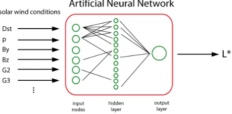
in the TSK03 magnetic field because of its simplicity. The drift shell model presented here is able to calculateL∗with less than 1% error compared to the original model but or-ders of magnitude times faster. (It is important to note here that no geomagnetic field model to date claims an accuracy even approaching 1% relative to the Earth’s actual dynamic magnetic field. The LANL∗calculation, like any other surro-gate model, is no better, but not measurably worse, than the model used to train it.) Figure 1 exemplifies a diagram of an artificial neural network used for our study.
3 Feedforward neural networks
Artificial neural networks are loosely based on the function of our nervous system in the sense that they represent a non-linear mapping from input to output signals (Bishop, 1995; Reed and Marks, 1999). They are a mathematical program-ming construct that mimic the behavior of biological neurons and are used to solve problems in machine learning and arti-ficial intelligence. They have proved useful for a number of real-world applications including credit scoring, fraud detec-tion, speech recognidetec-tion, and optical character recognition (OCR) just to name a few. Conceptually, an artificial neu-ral network consists of a number of non-linear processing units that are interconnected through weighted communica-tion lines. The units, called “neurons”, receive input signals from a number of other nodes and produce a single scalar
Fig. 1. Diagram for a layered feedforward neural network. Solar
wind conditions are used as input for predictingL∗ values. All nodes have a connection to every node from the previous layer but are not drawn here for simplicity. Also, not all possible parameters that can be used as input for the artificial neural network are shown. Specifically, our drift shell model includes additional values for Kp, solar wind density, velocity, and magnetic coordinates.
output which then can be used as input to other neurons via new weighted connections. In reality, a neural network is computed with several, simple matrix multiplications (Eq. 3). A very good overview of feedforward neural networks is pre-sented by Reed and Marks (1999).
Neural networks are usually organized in several layers. Such a network is also called a “multilayer perceptron”. The first layer provides a node for each input element (see Fig. 1). In our case the input layer consists of 15 nodes, one for each input parameter for the TSK03 model plus additional nodes for parameters that help to further specify the system (like ge-omagnetic coordinates). The hidden layer contains 20 neu-rons that are connected to each input node and one output node to produceL∗for a specified pitch angle.
The number of neurons in the hidden layer is somewhat arbitrary and usually has to be determined through testing. Too many neurons in the hidden layer can cause the artificial neural network to simply memorize patterns. In such a case the network will not be able to perform reliably with inputs that differ from those in the training set. Barron (1991, 1993, 1994) completed a study on how the error of a neural net-work output scales with the number of training samples and hidden nodes. He found that the error decreases ∝1/
√
N
as the number of training samples N increases. The error also decreases∝1/Mas a function of the number of hidden nodesM. In general, it has been shown, by e.g. Cybenko (1989), that a sufficiently large network is able to approx-imate any function with arbitrary accuracy (Bishop, 1995; Reed and Marks, 1999).
and a correct output (within a specified error) is obtained. Once the training of a neural network is completed, the output can be easily calculated given any set of input values. Ifxis the input vector, then the output vectoryin a 1-hidden-layer architecture is
y=f1W1f0W0x+b0+b1, (3) where the matricesW0,1denote the weight matrices of the
hidden and output layer andb0,1the bias vectors. The bias
vector is necessary to obtain a better classification but is, typ-ically, absorbed into the weight vector assuming that one of the inputs is constant (bias node).
The functionf is a non-linear squashing function applied to each component of a vector, for example
f (xi)= 1
1+e−xi. (4)
Squashing functions are used to limit very large positive or negative values. Sigmoid and tanh functions are also com-mon choices.
The interconnection weights (components of matrix W) are determined during training using an optimization algo-rithm which minimizes a chosen error function. Typically, training starts with a random choice of weights. The output (hereL∗) is calculated using Eq. (3) and compared to the “real”L∗(output from the Tsyganenko model). The error is calculated using, e.g., the mean-squared error
E= 1
P N
X
p X
i
dpi−ypi2, (5) wherep indexes the patterns in the training set, i indexes the output nodes, anddpiandypiare, respectively, the target and actual network output for the i-th output node on thep -th pattern. P andN are the number of training patterns and network outputs (Reed and Marks, 1999). Next, a different set of weights is chosen over and over again until the error is minimized for all input-output combinations (training pat-terns).
Because neural networks have such a redundant parallel structure, they exhibit some degree of fault tolerance. Many nodes draw information from a number of other nodes to pro-duce one overall output. This makes the system relatively in-sensitive to minor damage. The loss of some input degrades the system but does not necessarily lead to complete failure because the functions are distributed over several nodes in-stead of an isolated single location. This property has been called “graceful degradation” (Reed and Marks, 1999). Ex-amples for magnetic field models include Kp, Dst, solar wind velocityvsw and other input functions that are
corre-lated among each other. If one of the input parameters is not known or of bad quality, the input can be replaced with a default value and a reasonable output is still likely. This is in contrast to TSK03 which can only function with all input parameters available.
When neural networks are used as function approximators, they are typically used for interpolation and not extrapolation because the fit is usually good near the training data but poor elsewhere. This aspect of prediction accuracy is also called “generalization”. The distribution of training data and net-work complexity play an important role in the overall per-formance of the neural network. A poor set of training data may contain misleading regularities (Bishop, 1995; Reed and Marks, 1999). The best choice is to randomly select train-ing data followtrain-ing the same probability distribution that also governs future data.
Neural networks are not new to space physics and espe-cially space weather modeling. They have been used before to predict the relativistic electron flux at geosynchronous or-bit (Koons and Gorney, 1991), to forecast geomagnetic in-duced currents (Lundstedt, 1992), or to analyze solar wind data (Dolenko et al., 2001). To our knowledge, neural net-works have not previously been used as surrogate models re-placing complex space physics models such as global mag-netic field models.
4 The Tsyganenko 2003 Model
The magnetic field model TSK03 (Tsyganenko et al., 2003) is just one out of a series of models published by Tsyganenko and colleagues. The Tsyganenko magnetic field models are empirical models based on decades of magnetic field mea-surements. The models calculate quasi-static states of the Earth’s dynamic magnetic field based on solar wind condi-tions and geomagnetic indices. (The quasi-static state is a statistical average for a given set of solar wind conditions but is not a true equilibrium state.) TSK03 is one of the most accurate models currently available (Chen et al., 2007). It accounts for external contributions from the magnetotail cur-rent sheet, ring curcur-rent, magnetopause curcur-rent and Birkeland current (McCollough et al., 2008). It also includes partial ring current with field-aligned closure currents which allows it to account for local time asymmetries of the inner magneto-spheric field. These currents are driven by separate variables calculated as a time integral for a combination of geoeffec-tive parameters of solar wind density, speed, and the magni-tude of the southward component of the interplanetary mag-netic field (IMF). As with the actual geomagmag-netic field, the TSK03 model is compressed on the sunward side by the so-lar wind and extended on the antisunward side in a comet-like magnetic tail. The model also defines the boundary (a “magnetopause”) between the Earth’s geomagnetic field and the external solar wind fields. The properties are critical for particle motion and therefore for the calculation ofL∗.
Fig. 2. (left) Coordinate training ring for creating the training data set (left: top view; right: side view). Training coordinates are picked
randomly indicated by green star symbols. The quasi-parabolic black line (left) depicts the magnetopause which demarks the outer boundary between the geomagnetic field and the external solar wind.
time-integrated driving effect of the solar wind on the mag-netosphere (McCollough et al., 2008). Since our implemen-tation, the ONER-DESP library has changed names and is now called IRBEM-LIB.
5 Training the network
In order to create the training data, we have constructed an optimized algorithm that can compute a large number of
L∗ in a reasonably short period of time. The parallelized code can compute half a millionL∗training values typically within 45 h on a high-performance cluster at Los Alamos Na-tional Lab as compared to 900 h on a single CPU desktop machine with the standard implementation of the ONERA-DESP library.
The generalization performance of the neural network is how efficiently it can predict in untrained domains. The performance strongly depends on the selection of the train-ing data. Best results are obtained by randomly distributtrain-ing the input-output training patterns. This prevents the system from simply memorizing patterns in the input-output rela-tions. In order to test the neural network methodology we chose to train it for locations inside a coordinate ring with the following bounds: r∈[6.6RE,6.7RE], φ∈[−180◦,+180◦],
θ∈[−6◦,6◦] in spherical geographic coordinates. We
ran-domly picked 10 locations inside this coordinate ring (Fig. 2) to calculateL∗for every hour in the year 2002 using full
nu-merical integration of the TSK03 model with known solar wind and geomagnetic inputs. This resulted in 87 600 input-output patterns that we used to train the neural network. The input data for Kp, Dst, solar wind density, pressure, velocity,
y andzcomponents of the IMF magnetic field were taken from the omni2 data set provided by NASA via OMNIWeb (http://omniweb.gsfc.nasa.gov/).
Typically, the locations inside the coordinate training ring are on closed drift shells. L∗is only defined when the inte-gral is closed. However, during storm conditions the
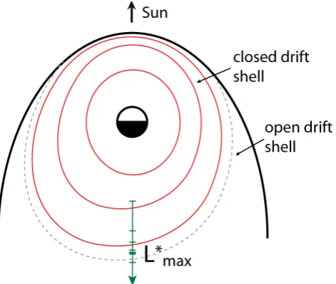
magne-Fig. 3. Conceptual diagram of finding the last closed drift shell
by using a bisection search algorithm along the radial direction at midnight local time. The dashed line represents the last closed drift shell withL∗max.
tosphere can be compressed by the solar wind and the drift shells move outward due to adiabatic effects and end up as open drift shells for which the integral of the magnetic flux
8(Eq. 2) is not defined. During the main phase of a storm the increase in ring current causes a decrease in the magnetic field strength in the inner magnetosphere and a reduction of the magnetic flux enclosed by an electron drift orbit (Kim and Chan, 1997; Roederer, 1970). This effect requires two sep-arate neural networks, one that can tell us the maximumL∗
Fig. 4. Set of neural networks that can calculateL∗as a function of pitch angle. Each set consists of several neural networks for a range of pitch angles. One set calculatesL∗and the other set computes the last closed drift shellL∗max. The coordinates of the geosynchronous spacecraft are represented by Lm and MLT.
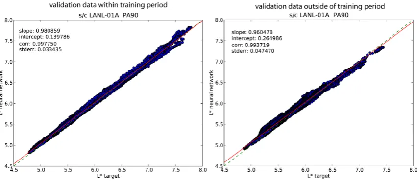
Fig. 5. Validation for the neural network using an out-of-sample data set from the positions of LANL-GEO spacecraft LANL-01A for 90
degrees pitch angle. Each point represents oneL∗calculation by the Tsyganenko model versus the neural networkL∗result. The dashed green line would represent a perfect prediction by the neural network; the red line is a linear fit to the predictions. The standard deviation is1L∗≈0.04 or less than 1%. (left) Validation data is from the same year as the training data period of 2002. (right) Validation data from 2001 and 2005 was not part of the training data period.
We trained the first neural network NN-1 withL∗maxvalues calculated from the full integration of the TSK03 magnetic field model. We have used a bisection search algorithm to find the last valid closed drift shell. We calculateL∗ along the radial coordinate at midnight local time (Fig. 3) stepping outwards until a bad value is found. Then we step back in-wards and outin-wards at smaller increments until sufficient ac-curacy is achieved. Solar wind data including Dst and Kp were used as input and the obtainedL∗maxvalues were used as target for training the network. The training region we described earlier does not apply to this part of the neural
net-work since the last closed drift shellL∗maxis a global value. We trained the second neural network NN-2 with theL∗
Fig. 6. Histogram plot of the error introduced by using the neural network. (left) Validation data is from the same year as the training data
period of 2002. (right) Validation data from 2001 and 2005 was not part of the training data period.
10 20 30 40 50 60 70 80 90 PA in [deg]
0.044 0.046 0.048 0.050 0.052 0.054 0.056 0.058 0.060 0.062
std. dev. in [L*]
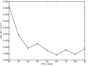
Fig. 7. The change in standard deviation using out of sample
val-idation data as a function of pitch angle. The error of the neural network gradually increases towards lower pitch angles.
of pitch angleα. Since the results from NN-1 and NN-2 de-pend on the pitch angle, it was necessary to create several neural networks for a range of pitch angles.
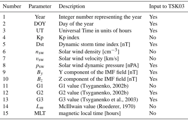
The setup of neural networks is displayed in Fig. 4. Each set consists of nine neural networks, one for each chosen pitch angle. One set (NN-1) is for calculating the last closed drift shellL∗maxand the second set (NN-2) is for calculating the actualL∗ value. We have also added several more pa-rameters than the ones actually required by TSK03 (see Ta-ble 1). We found that these additional values, including Kp, solar wind density, velocity, G1, and especially magnetic co-ordinates (MacIllwain L, magnetic local time) dramatically increase the generalization properties of the neural network.
We used the python module ffnet (Wojciechowski, 2007) to train our neural networks with optimization algorithm pro-vided in the ffnet package. The ffnet python module has a functionality that allows exporting the trained neural network into a FORTRAN subroutine which then enables us to share the neural network efficiently.
Fig. 8. Test case of calculatingL∗ with the Tsyganenko model TSK03 (blue) and with the neural network (red) for satellite LANL-01A. The standard deviation error is1L∗≈0.04 or less than 1% for 90 degrees pitch angle. The time is give in units of hours since the beginning of 2002.
The resulting set of neural networks can calculateL∗ in a fraction of the time required by full drift shell integration. Half a million calculations can be done in only a few seconds whereas running the magnetic field model in serial mode would have taken over 1700 h. This translates into a speedup of over several million times. These numbers are only for the actualL∗ calculations. In reality, one still has to pre-pare the data, perform coordinate transformations and single field line integrations for obtaining the adiabatic coordinate
Table 1. Input parameters for the neural network LANL∗.
Number Parameter Description Input to TSK03
1 Year Integer number representing the year Yes
2 DOY Day of the year Yes
3 UT Universal Time in units of hours Yes
4 Kp Kp index No
5 Dst Dynamic storm time index [nT] Yes
6 nsw Solar wind density [cm−3] No
7 vsw Solar wind velocity [km/s] No
8 psw Solar wind dynamic pressure [nPA] Yes
9 By Y component of the IMF field [nT] Yes 10 Bz Z component of the IMF field [nT] Yes
11 G1 G1 value (Tsyganenko, 2002b) No
12 G2 G2 value (Tsyganenko, 2002b) Yes
13 G3 G3 value (Tsyganenko et al., 2003) Yes 14 Lm McIllwain value (Roederer, 1970) No
15 MLT magnetic local time [hours] No
Fig. 9. The generalization properties of the neural network shows
how far the neural network can extrapolate into regions that were not part of the training coordinate ring. We plot the average dif-ference between the target and the neural network L∗ and find that although the training coordinates were very limited to geosyn-chronous orbit atr≈6.6 the neural network is able to give compa-rable results between 5.8<r<7.3RE. The gray area represents the overall accuracy of the neural network,1L∗=0.047, when com-pared to data from inside the training region.
6 Testing and validating the network
We validated our neural network by comparing its results to the results from the full numerical integration of the actual magnetic field model. We chose a number of LANL geosyn-chronous satellites and calculated theirL∗ values in hourly resolution covering the years of 2002 and partially 2001 and 2005. The validation results of the neural network of this out-of-training-sample are shown in Figs. 5 and 6. We have
split the validation data for comparing the results from (i) us-ing the same time period and solar wind conditions of 2002 but with different geographic coordinates than the training coordinates and (ii) using the different solar wind conditions of the years 2001 and 2005. We have tested and validated the neural network with coordinates from several geosyn-chronous satellites and found similar performance with all of them. Figures 5 and 6 show one validation example with the satellite LANL-01A. In Fig. 5,L∗values of the neural
net-work are plotted against the actual results from using TSK03 for conditions in 2002 (training period) and 2001, 2005 (out-side of the training period). Figure 6 shows the distribution of errors related to the difference between the neural network results and the full integration of the TSK03 model. We find the standard deviation error is1L∗≈0.04 or less than 1%. For off-equatorial pitch angles the standard deviation can be larger to about1L∗≈0.06 (see Fig. 7). This is much lower than the intrinsic error of empirical magnetic field models (Huang et al., 2008) which is estimated to be up to 50% during geomagnetic storms and shows that using the neural network will add only a marginal error for greatly enhanced performance. The overall error is calculated by adding the variances: σTSK032 +σN N2 =σtot2. We also show in Fig. 8 that the neural networkL∗is indeed following theL∗calculation from using TSK03 on a point by point time series.
The complete library of neural networks plus ex-amples are included as supplemental material to this publication (http://www.geosci-model-dev.net/2/113/2009/ gmd-2-113-2009-supplement.zip). After extracting the files, read the “README” file and follow the instructions of us-ing the Makefile and adoptus-ing your FORTRAN compiler. In-structions for calling the library from IDL are included as well.
7 Conclusion and summary
We have presented a new, computationally efficient method of calculating the magnetic adiabatic invariant integral,L∗. Space weather models for the inner magnetosphere use adi-abatic invariants to describe charged particle motion in re-duced ”magnetic coordinates” that are used in models of the space environment. In particular, models of the radiation belt environment use the adiabatic coordinateL∗to study the ac-celerating, transport, and scattering of radiation belt particles in order to better understand radiation effects on satellites.
Computationally efficientL∗calculations are particularly important for space weather applications that have to process data in real-time and for those that require time-dependent models spanning one or more 11-year solar activity cycles. Both applications of radiation belt models are currently be-ing developed for operational use but that development has previously been hindered by the long computation times re-quired for full numerical integration of modern, sophisticated models of the Earth’s geomagnetic field.
By using a feedforward neural network as a surrogate model and training it with full numerical integration of the TSK03 geomagnetic field model, we have demonstrated that we can reproduce the TSK03L∗values with accuracies that are on the order of 1%. This is to be contrasted with a 10– 50% inherent uncertainty of the TSK03L∗value relative to the actual geomagnetic field. The technique we have pre-sented, however, is general and can be applied to any ge-omagnetic field model, including any future models with higher inherent accuracy and with arbitrary levels of com-plexity.
The ability to efficiently calculate L∗ with insignificant additional loss of accuracy is fundamentally important for coupling state-of-the-art geomagnetic field models with next-generation radiation belt and space environment models. That coupling will enable better understanding of the physi-cal processes that control the space environment, better spec-ification and prediction of the environment for satellite de-signers and operators, and ultimately more reliable and cost-effective design and operation of the satellites upon which our society increasingly depends.
While the current version (V 1.0) of the LANL∗library has only been trained and validated for the region near geosyn-chronous orbit, we are actively working on extending the neural network training to include the whole inner
magne-tosphere. Codes applicable to the entire near-Earth space en-vironment will be published in a future version of the LANL∗
library.
Acknowledgements. This work has been supported by Los
Alamos National Laboratory’s LDRD Directed Research Program (DREAM) and the National Science Foundation (grant 0718710).
Edited by: D. Lunt
References
Barron, A.: Approximation Bounds For Superpositions Of A Sig-moidal Function, Information Theory, IEEE Transactions on, 85–85, 1991.
Barron, A.: Universal approximation bounds for superpositions of a sigmoidal function, Information Theory, IEEE Transactions on, 39, 930–945, 1993.
Barron, A. R.: Approximation and estimation bounds for artificial neural networks, Mach. Learn., 14, 115–133, doi:10.1007/BF00993164, 1994.
Beutier, T. and D. Boscher: A three-dimensional analysis of the electron radiation belt by the Salammbˆo code, J. Geophys. Res., 100, 14853–14862, 1995.
Bishop, C. M.: Neural networks for pattern recognition, Clarendon Press, Oxford University Press, Oxford, New York, 1995. Boscher, D., Bourdarie, S., O’Brien, P., and Guild, T.:
ONERA-DESP library V4.1, http://irbem.sourceforge.net/, 2007. Chen, Y., Friedel, R. H. W., Reeves, G. D., Cayton, T. E., and
Chris-tensen, R.: Multisatellite determination of the relativistic elec-tron phase space density at geosynchronous orbit: An integrated investigation during geomagnetic storm times, J. Geophys. Res., 112, 1–16, 2007.
Cybenko, G.: Approximation by superpositions of a sig-moidal function, Math. Control Signal., 2, 303–314, doi:10.1007/BF02551274, 1989.
Dolenko, S., Orlov, Y., Persiantsev, I., and Shugai, Y.: Neural Net-work Analysis of Solar Wind Data, Applied Problems in Systems of Patttern Recognition and Image Analysis, 11, 296–299, 2001. Huang, C.-L., Spence, H. E., Singer, H. J., and Tsyganenko, N. A.: A quantitative assessment of empirical magnetic field models at geosynchronous orbit during magnetic storms, J. Geophys. Res. (Space Physics), 113, A04208, doi:10.1029/2007JA012623, 2008.
Kim, H.-J. and Chan, A. A.: Fully adiabatic changes in storm time relativistic electron fluxes, J. Geophys. Res., 102, 22107–22116, 1997.
Kleijnen, J. P. C.: Design and analysis of simulation experiments, International series in operations research and management sci-ence, 111, Springer, New York, 2008.
Koons, H. C. and Gorney, D. J.: A neural network model of the rel-ativistic electron flux at geosynchronous orbit, J. Geophys. Res., 96, 5549–5556, 1991.
Lundstedt, H.: Neural networks and predictions of solar-terrestrial effects, Planet. Space Sci., 40, 457–464, 1992.
Myers, R. H. and Montgomery, D. C.: Response surface method-ology process and product optimization using designed experi-ments, Wiley, New York, Chichester, 2002.
Olson, W. P. and Pfitzer, K. A.: Magenetospheric magnetic field modeling, Annual Scientific Report, 1977.
Queipo, N. V., Haftka, R. T., Shyy, W., Goel, T., Vaidyanathan, R., and Kevin Tucker, P.: Surrogate-based analysis and optimization, Prog. Aerosp. Sci., 41, 1–28, 2005.
Reed, R. D. and Marks, R. J.: Neural smithing: supervised learning in feedforward artificial neural networks, The MIT Press, Cam-bridge, Mass., 1999.
Reeves, G., Friedel, R., Chen, Y., Koller, J., and Henderson, M.: The Los Alamos Radiation Environment Assimilation Model (DREAM) for Space Weather Specification and Forecasting, in Advanced Maui Optical and Space Surveillance Technologies Conference. 2008.
Roederer, J. G.: Dynamics of geomagnetically trapped radiation, Physics and chemistry in space, Vol. 2, Springer-Verlag, Berlin, New York, 1970.
Rumelhart, D. E., Hinton, G. E., and Williams, R. J.: Learning rep-resentations by back-propagating errors, Nature, 323, 533–536, doi:10.1038/323533a0, 1986.
Schulz, M.: The magnetosphere, Geomagnetism, 4, 87–293, 1991. Schulz, M. and Lanzerotti, L. J.: Particle diffusion in the radiation
belts, Physics and chemistry in space, Vol. 7, Springer-Verlag, Berlin, New York, 1974.
Tsyganenko, N. A.: A model of the near magnetosphere with a dawn-dusk asymmetry 1. Mathematical structure, J. Geophys. Res. (Space Physics), 107, 1179, doi:10.1029/2001JA000219, 2002a.
Tsyganenko, N. A.: A model of the near magnetosphere with a dawn-dusk asymmetry 2. Parameterization and fitting to observations, J. Geophys. Res. (Space Physics), 107, 1176, doi:10.1029/2001JA000220, 2002b.
Tsyganenko, N. A. and Sitnov, M. I.: Modeling the dynam-ics of the inner magnetosphere during strong geomagnetic storms, J. Geophys. Res. (Space Physics), 110, A03208, doi:10.1029/2004JA010798, 2005.
Tsyganenko, N. A., Singer, H. J., and Kasper, J. C.: Storm-time distortion of the inner magnetosphere: How severe can it get?, J. Geophys. Res. (Space Physics), 108, 1209, doi:10.1029/2002JA009808, 2003.
Wojciechowski, M.: ffnet: Feed-forward neural network for python, http://ffnet.sourceforge.net/, 2007.