www.geosci-model-dev.net/7/1945/2014/ doi:10.5194/gmd-7-1945-2014
© Author(s) 2014. CC Attribution 3.0 License.
Direct numerical simulations of particle-laden density currents with
adaptive, discontinuous finite elements
S. D. Parkinson1, J. Hill1, M. D. Piggott1,2, and P. A. Allison1
1Applied Modelling and Computation Group, Department of Earth Science and Engineering, South Kensington Campus,
Imperial College London, London SW7 2AZ, UK
2Grantham Institute for Climate Change, South Kensington Campus, Imperial College London, London SW7 2AZ, UK
Correspondence to: S. D. Parkinson ([email protected])
Received: 2 April 2014 – Published in Geosci. Model Dev. Discuss.: 7 May 2014 Revised: 30 July 2014 – Accepted: 5 August 2014 – Published: 5 September 2014
Abstract. High-resolution direct numerical simulations (DNSs) are an important tool for the detailed analysis of turbidity current dynamics. Models that resolve the vertical structure and turbulence of the flow are typically based upon the Navier–Stokes equations. Two-dimensional simulations are known to produce unrealistic cohesive vortices that are not representative of the real three-dimensional physics. The effect of this phenomena is particularly apparent in the later stages of flow propagation. The ideal solution to this prob-lem is to run the simulation in three dimensions but this is computationally expensive.
This paper presents a novel finite-element (FE) DNS tur-bidity current model that has been built within Fluidity, an open source, general purpose, computational fluid dynamics code. The model is validated through re-creation of a lock release density current at a Grashof number of 5×10⁶ in two and three dimensions. Validation of the model consid-ers the flow energy budget, sedimentation rate, head speed, wall normal velocity profiles and the final deposit. Conser-vation of energy in particular is found to be a good metric for measuring model performance in capturing the range of dynamics on a range of meshes. FE models scale well over many thousands of processors and do not impose restrictions on domain shape, but they are computationally expensive. The use of adaptive mesh optimisation is shown to reduce the required element count by approximately two orders of magnitude in comparison with fixed, uniform mesh simula-tions. This leads to a substantial reduction in computational cost. The computational savings and flexibility afforded by adaptivity along with the flexibility of FE methods make this model well suited to simulating turbidity currents in complex domains.
1 Introduction
Density currents, also known as gravity or buoyancy cur-rents, occur when two fluids with different densities meet. The density difference creates a pressure gradient that causes the more dense fluid to intrude beneath the less dense fluid. They occur in both natural and man-made situations, within a wide range of environments, and over a vast range of tem-poral and spatial scales. When a fluid contains particles in suspension the bulk density of that fluid changes. Density currents that are at least partly driven by a density variation due to suspended particles are termed particle-laden density currents. Examples include pyroclastic flows, dust storms, avalanches and turbidity currents.
component of the stratigraphic record, and their deposits can form hydrocarbon reservoirs (Kneller and Buckee, 2000; Sequeiros et al., 2009). Having a good understanding of tur-bidity current behaviour can also allow us to predict and im-prove water quality in reservoirs by enhancing our under-standing of pollutant concentrations (Alavian et al., 1992; Huang et al., 2005) and oxygenation (Best et al., 2005).
Studying turbidity currents is not easy. They occur infre-quently and unpredictably at any particular location, and tend to destroy any measurement devices that are positioned to measure their effects. The dynamics of these currents are highly complex, with strong feedback between turbulence and sediment suspension making measurement of the dy-namics difficult (Kneller and Buckee, 2000; Serchi et al., 2012). Small-scale laboratory experiments can provide use-ful insight into the dynamics of these currents, but are limited by scaling issues and the available measurement techniques (Kneller and Buckee, 2000).
High-resolution numerical models have become an im-portant tool for the detailed analysis of particle-laden den-sity current dynamics. Models that resolve the vertical struc-ture of the flow are typically based upon the Navier–Stokes equations. Direct numerical simulations (DNSs) of particle-laden density currents should be carried out in three sions as unrealistic cohesive vortices form in two dimen-sions that have a significant impact on virtually all of the important outputs from these simulations (Cantero et al., 2007; Espath et al., 2014). The scale of particle-laden density currents is often described using the Grashof number. The Grashof number approximates the ratio of buoyant to vis-cous forces. This is equivalent to the square of the Reynolds number of a flow where the buoyancy velocity is used as the characteristic velocity. DNS modelling of particle-laden den-sity currents has been achieved in three dimensions at mod-erate Grashof numbers of O 106
by Necker et al. (2002) and Nasr-Azadani and Meiburg (2011). Espath et al. (2014) have simulated a particle-laden density current at a Grashof number ofO 108. Computational power has limited mod-elling of higher Grashof number flows. A Grashof number ofO 108translates into modelling of low volumetric parti-cle concentration 10−4–10−3% flows in water at laboratory scales. Even at these moderate Grashof numbers a fully tur-bulent flow is obtained (Necker et al., 2002; Espath et al., 2014), and very useful insights have been obtained from sim-ulations of particle-laden currents within this range.
There has been some success in modelling these flows using DNS in two dimensions which makes the problem more computationally tractable (Blanchette et al., 2005; Ooi et al., 2007). However, Espath et al. (2014) showed that the only important diagnostic that can be accurately predicted using a two-dimensional DNS model is the sedimentation rate. Another alternative to three-dimensional DNS is to use turbulence models to handle the small-scale turbulence and only resolve the large-scale motions. Turbulence modelling
is undoubtedly important for extending models that resolve the vertical structure of the flow to more realistic Grashof numbers. Whether it is appropriate to use a turbulence model depends upon the diagnostics that are important in the study. DNS simulations are necessary to perform detailed analysis of turbulent structures, and also for the validation of turbu-lence models for this application.
DNS models of turbidity currents in three dimensions have generally been formulated using spectral element tech-niques (Necker et al., 2002) and finite differences (Espath et al., 2014; Nasr-Azadani and Meiburg, 2011). These models are designed to be highly efficient, having struc-tured meshes and, in most cases, high-order methods such that these computationally challenging problems become tractable. However, these computationally optimised meth-ods make simulations in irregularly shaped domains very dif-ficult (Mohd-Yusof, 1998). Natural turbidity currents propa-gate over complex bathymetries. The interaction of turbid-ity currents over complex geometries is therefore of obvi-ous interest. The model of Nasr-Azadani and Meiburg (2011) can model turbidity currents in geometries with some com-plex features using the immersed boundary method, but this method has limitations and is not suitable for all use cases (Mohd-Yusof, 1998).
2 Mathematical model 2.1 Governing equations
A general discussion of particle motion in a non-uniform flow by Maxey and Riley (1983) stated that pressure gradient, added mass, viscous Stokes and augmented drag, and buoy-ancy forces need to be considered. This work considers flows where the particles are very small in relation to the length scales of motion. It also considers situations where the parti-cle density is significantly larger than that of the surrounding fluid. For example, silica is≈2.6 times the density of water in turbidity currents, and ≈2600 times the density of air in dust storms. Based upon these restrictions Maxey and Riley (1983) showed that the dominant forces in the equations of motion for a single particle relative to the fluid in which it is suspended are the viscous Stokes drag and buoyancy terms.
Particle-laden density currents consist of a collection of particles and hence particle collisions must also be consid-ered. The effect of these collisions can be safely ignored by limiting the model to applications where the sediment vol-ume fraction is less than 1 % (Necker et al., 2002). Floccula-tion of sediment particles can be ignored if the model is fur-ther restricted to sediment sizes of sand and larger (>64 µm) (Maerz et al., 2011).
Cantero et al. (2008) showed that the effects of inertia on particle motion in density currents are insignificant for parti-cles smaller than 250 µm in diameter and hence the model is restricted to sediment diameters below 250 µm.
Taking all of the above into account, the acceleration of particles will be the same as that of the containing fluid. Particles will move with a velocity equal to the sum of the fluid velocity, u˜, and a settling velocity, u˜sk, where ∼
de-notes a dimensional value. The settling speed, u˜s, is
ob-tained by balancing the Stokes drag and buoyancy forces, and
k=(0,0,1)T. This means that the evolution of the particle volume fraction,c˜, can be described with a transport equa-tion of the form
∂c˜
∂t˜+(u˜i− ˜uski)
∂c˜
∂x˜i
= ˜κ ∂
2c˜
∂x˜i∂x˜i
, (1)
whereκ˜is the particle concentration diffusivity. Particle con-centrations will never be completely uniform. Individual par-ticles will have a range of masses and settling velocities which lead to slight variations in speed and trajectory. As particles move past one another they interact and cause a self-induced hydrodynamic diffusion (Davis and Hassen, 1988). The magnitude of this diffusivity is generally chosen to be 0.7–1.0 times the ambient fluid viscosity (Necker et al., 2002; Cantero et al., 2008). Higher values help convergence and stability of the solution. It has been shown that this value has little effect on the relevant flow quantities so long as it does not significantly exceed the ambient fluid viscosity (Hartel et al., 2000).
Continuity and momentum balance in this model is gov-erned by the Navier–Stokes equations. The fluid is assumed to be incompressible. Due to the very low volumetric concen-trations, the displacement of fluid by the suspended particles can be ignored (Necker et al., 2002). Therefore the velocity field is considered to be divergence free. The Boussinesq ap-proximation is adopted, in which density is considered con-stant except in the buoyancy term. The isotropic kinematic viscosity,ν˜, is assumed constant throughout the model. This leads to the following form for the Navier–Stokes equations:
∂u˜i
∂t˜ + ˜uj
∂u˜i
∂x˜j = −
∂p˜
∂x˜i − ˜g 0k
i+
∂ ∂x˜j
˜
Sij, (2a)
∂u˜i
∂x˜i
=0, (2b)
where the stress tensor,S, for an incompressible flow is de-˜ fined as
˜
Sij= ˜ν
∂u˜
i
∂x˜j +∂u˜j
∂x˜i
, (3)
and the buoyancy density,g˜0, is a function of the sediment density,ρc, the ambient fluid density,ρa, the magnitude of
the acceleration due to gravity,g˜, and the volumetric con-centration of sediment,c˜, with the form
˜
g0=ρ˜c− ˜ρa ˜
ρa ˜
gc .˜ (4)
The assumptionc˜1 and (ρ˜c− ˜ρa)/ρ˜a=O(1)justify the
use of the Boussinesq approximation.
Particle-laden density currents deposit and/or erode the surface over which they travel. This means that the suspended mass changes with time, i.e. they are non-conservative. They have the potential to accelerate if their mass increases, or decelerate more rapidly due to settling out of the suspended sediment. The dynamics of sediment ero-sion are complex. Sediment on the bed will affect turbulence in the boundary layer. Larger sediment grains will shield smaller ones and grains may adhere to each other in the bed. The bed shape will also change as sediment is eroded, gen-erating complex topography that may promote or inhibit fur-ther sediment erosion. Empirical algorithms have been de-veloped for predicting erosion rates based upon particle pa-rameters and the bed shear stress. Erodible boundaries,0d, are modelled here as a flux boundary condition of the form
niκ˜
∂c˜
∂x˜i
= ˜usE˜on0d, (5)
whereE˜is the non-dimensional erosion rate of sediment into suspension,nis the boundary unit normal vector.
sediment in finite size ranges. They validated these against laboratory results, and produced an improved formula for sediment erosion. This has been successfully used in work by Huang et al. (2007) and Sequeiros et al. (2009) when mod-elling sediment-laden density currents and is described as
˜
E= A
˜
Z5
1+AZ˜5/0.3 , (6a)
˜ Z= √ ˜ τb ˜ us s ˜
ρc− ˜ρa ˜
ρa ˜
gd˜
d˜ ˜
ν
!0.6
, (6b)
whereA=1.3×10⁻⁷is a non-dimensional constant andd˜is
the diameter of the suspended sediment. The bed shear stress,
˜
τb, is defined as ˜
τb=
ni ˜ Sij . (7)
The total flux through an erodible boundary is calculated as
∂η˜
∂t˜ =niu˜skic˜b− ˜us ˜
E, (8)
whereη˜is the depth of the deposited sediment in the bed and
˜
cb is the volumetric concentration of sediment at the
sedi-ment bed boundary. E˜ is limited such that it never exceeds
˜
η/1t, where1tis the period of a time step. As in the work by Necker et al. (2002) and Espath et al. (2014), no adjust-ment for porosity of the deposit is included.
It is also possible for sediment to be moved along the bed without being entrained into the flow. This process is known as bedload transport. This has not been included in the cur-rent work. Sequeiros et al. (2009) stated that suspended sed-iment is the key factor in the movement of sedsed-iment in tur-bidity currents and that bedload transport can be neglected for currents that do not have a significant fraction of particles larger than 100 µm.
Four parameters are used to non-dimensionalise the equa-tions outlined above:
Gr= u˜b ˜ h0 ˜ ν !2 , (9)
Sc=ν˜ ˜
κ , (10)
us= ˜
us ˜
ub
, (11)
Rp=
s ρ˜
c− ˜ρa ˜
ρa ˜
gd˜
d˜ ˜
ν , (12)
where Gr is the Grashof number, Sc is the Schmidt number,
Rp is the particle Reynolds number, andh0 is a
character-istic length scale (half the lock-release depth in this work, as defined in Sect. 3). The buoyancy velocity,u˜b, is used as
the characteristic velocity scale and is defined in terms of the initial buoyancy density,g˜00, and the characteristic lengthh0,
as
˜
ub=
q
˜
g00h˜0. (13)
Equations (1)–(3) and (5)–(8) can now be redefined in non-dimensional form as
∂c
∂t +(ui−uski) ∂c ∂xi =
1 p
Sc2Gr ∂2c
∂x2i , (14)
∂ui
∂t +uj ∂ui
∂xj = − ∂p
∂xi −kic+ ∂
∂xjSij, (15)
∂ui
∂xi =0, (16)
ni
1 p
Sc2Gr ∂c
∂xi =usEon0
d, (17)
E= A Z
5
1+AZ5/0.3 , (18)
Z= √
τb
us
R0.6p , (19)
τb=
niSij
, (20)
∂η
∂t =niuskicb−usE, (21)
Sij=
1 √ Gr ∂u i ∂xj
+∂uj
∂xi
. (22)
2.2 Discretisation
as streamline-upwinding (Peraire and Persson, 2008). DG methods also work well on arbitrary meshes and have the desirable properties of having a block-diagonal mass matrix that can be trivially inverted locally for each element. This al-lows for certain equations to be solved very efficiently (Bassi and Rebay, 1997).
Use of the DG method requires a choice of flux schemes for both the advective and diffusive terms. A simple upwind flux is chosen for advective terms. A centred flux is used for the diffusive terms. The compact discontinuous Galerkin method (CDG) is used to implement the diffusive terms (Peraire and Persson, 2008). For a detailed discussion of DG discretisations and flux terms see the review paper by Cockburn and Shu (2001).
Advection when using a DG discretisation is not bounded. Undershoots and overshoots can occur that affect the dy-namics of a gravity current. Slope limiters are employed to bound the solution although these can be dissipative. Vertex-based slope limiting, as suggested by Kuzmin (2010), is used herein.
For the pressure field a quadratic continuous Galerkin scheme is used. We therefore have a mixed finite element pairing for solving the incompressible Navier–Stokes equa-tions. This element pairing, described by Cotter et al. (2009), has the benefit of satisfying the Ladyženskaja–Babuška– Brezzi (LBB) stability condition and hence needs no sta-bilisation of the pressure field. Additionally, a higher-order-accurate pressure field means that the pressure gradient term in the momentum equation has the same order of accuracy as the buoyancy forcing term. These two terms dominate in early stages of propagation and hence the ability for these terms to balance is important in determining how the flow evolves.
A Crank–Nicolson time discretisation is used throughout the model which is second-order accurate in time. The cou-pled system of non-linear equations are solved using two non-linear iterations known as Picard iterations. Within each non-linear iteration the equations are linearised using the best available solution for each variable that is not being solved for. The momentum and conservation equations are solved using a pressure correction scheme.
An adaptive time step is used. This makes the simulation more robust when using a changing multi-scale mesh and also takes advantage of the reducing current velocity over time which allows for much larger time steps towards the end of the simulation. The time step length is based upon obtaining a target Courant number of 2. This is a relatively conservative requirement for the implicit time discretisation used.
There are two exceptions to the use of Crank–Nicolson time discretisation. Slope limiters used with DG discretisa-tions only guarantee a bounded solution in conjunction with an explicit advection scheme. Therefore the sediment trans-port and momentum equations are solved in two stages. Ad-vection is calculated using explicit subcycles with adaptive
time step lengths based upon achieving a Courant num-ber of 0.2 (an order of magnitude smaller than the rest of the model). Diffusion/viscous dissipation is solved using the simulation time step,1t, and a Crank–Nicolson discretisa-tion. Additionally, the bed shear stress is calculated at the start of each time step and hence the erosion rate is totally explicit. A thorough description of the time discretisation outlined above is available in the Fluidity manual (Imperial College London AMCG, 2014).
2.3 Anisotropic mesh adaptivity
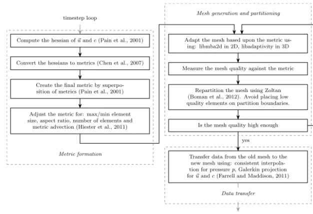
The motivation behind using mesh adaptivity is to optimise the spatial resolution with time such that both the discreti-sation error and computational cost of a simulation are min-imised (Piggott et al., 2005). Adapting the mesh is split into three tasks. The first step is to determine the desired edge lengths, or to form a metric against which element edge lengths can be defined, the second part involves generating a new mesh that better fits these requirements and distribut-ing this mesh amongst the active processors, and the third involves transferring data from the old mesh to the new mesh (see Fig. 1). A brief description of each phase of the pro-cess is included below. The reader is referred to the work of Piggott et al. (2008) for more details.
2.3.1 Metric formation
Determining the desired edge lengths for a mesh requires some quantification of the error in the solution due to spa-tial discretisation. This is difficult to do as there is usually no better estimate of the exact solution than the estimate from the current discretisation. An indirect method of measuring the error is required. Ciarlet (1991) showed that the finite ement error can be bounded by the interpolation error for el-liptic problems. It is assumed that this also holds for other partial-differential equations. This is deemed a reasonable way of defining an error indicator (Fortin, 2000).
The aim is to minimise the error in fields that are dis-cretised using first-order discretisations. For first-order el-ements, the interpolation error depends upon the Hessian, H (the matrix of second-order partial derivatives) (Frey and Alauzet, 2005). The second derivative of such a discretisa-tion is formally zero and hence some method of recovering the Hessian for these fields is needed. In Fluidity a double-lumped Galerkin projection is used to compute the Hessian as described by Pain et al. (2001). This Hessian will contain information about both the magnitude and direction of the curvature of a field and hence can be used to guide genera-tion of anisotropic elements. This is very useful in regions, such as boundary layers, where the solutions vary signifi-cantly more rapidly in one direction than in others.
Compute the hessian of~uandc(Pain et al., 2001)
Convert the hessians to metrics (Chen et al., 2007)
Create the final metric by superpo-sition of metrics (Pain et al., 2001)
Adjust the metric for: max/min element size, aspect ratio, number of elements and metric advection (Hiester et al., 2011)
Adapt the mesh based upon the metric us-ing: libmba2d in 2D, libadaptivity in 3D
Measure the mesh quality against the metric
Repartition the mesh using Zoltan (Boman et al., 2012). Avoid placing low quality elements on partition boundaries.
Is the mesh quality high enough
Transfer data from the old mesh to the new mesh using: consistent interpola-tion for pressurep, Galerkin projection for~uandc(Farrell and Maddison, 2011)
yes
no timestep loop
timestep loop
Metric formation
Mesh generation and partitioning
Data transfer
Figure 1. A description of the high-level algorithm involved in adapting the mesh. This algorithm is invoked repeatedly throughout the simulation at a fixed interval specified as a number of time steps.
measured against it: q
viMijvj=1 ∀v∈M. (23)
The choice of formulation for M is therefore fundamental to the way in which the mesh adapts. A formulation suggested by Chen et al. (2007) which controls theL2norm of the in-terpolation error is used:
M=1
εdet|H|
− 1
4+n|H|, (24)
wherenis the number of dimensions, andεis the interpola-tion error bound, a value which is defined by the user. ForLp
methods, Loseille and Alauzet (2011) foundp=2 to be the optimal value and incorporate more influence from dynam-ics of smaller magnitudes. Experience has shown this metric formation to be very effective for gravity current simulations (Hiester et al., 2011, 2014).
It is often important to adapt to more than one solution field. When this is the case the final metric is a superposition of the metrics calculated for each individual field (Pain et al., 2001). At this point the metric is also modified to take into account bounds upon the maximum and minimum element size, maximum allowable aspect ratio, edge length gradation, and the number of elements. Additionally, this metric can be advected forward in time providing an estimate of future requirements for the mesh resolution and allowing for more time between adapt operations (Hiester et al., 2011). 2.3.2 Mesh generation and partitioning
The second stage of creating the new mesh is handled by the open-source mesh optimisation library libmba2d in two
dimensions, or libadaptivity, another open source library de-veloped alongside Fluidity, in three dimensions. This in-volves a series of topological and geometrical operations, with the aim of obtaining a mesh with unit edge lengths with respect to the determined metric, see Eq. (23). These oper-ations include node insertion or deletion, edge/face swap-ping, which preserves the node locations but manipulates edge lengths by changing the configuration of a edge/face between elements, and node movement (Piggott et al., 2009). The Zoltan library (Boman et al., 2012) is used to partition the mesh in parallel after each adapt iteration. Nodes cannot be adapted at the edge of partitions. After each adapt iteration parameters are passed to the Zoltan library which discour-age it from generating partitions through elements that have not been able to adapt. For three-dimensional simulations, a minimum of three adapt iterations are required to allow all elements to adapt and create a mesh that satisfies the metric constraint everywhere. Zoltan’s graph re-partitioning algo-rithm is used to partition the mesh efficiently between adapt iterations. Once a good quality mesh has been obtained the hypergraph partitioning method is used to redistribute the el-ements amongst the processes.
2.3.3 Data transfer
After creating the new mesh the data are transferred on to it from the previous mesh. For the purposes of describing this step these meshes will be referred to as the target and donor meshes respectively.
Consistent interpolation is very cheap and hence is a good choice for data transfer of this field.
All other prognostic fields are discontinuous. Consistent interpolation cannot be used for discontinuous fields as test and trial functions are not continuous across element bound-aries. Additionally, consistent interpolation is not conserva-tive and is dissipaconserva-tive. It is important to conserve sediment mass during data transfer. It is also important that dissipa-tion of both velocity and sediment is kept to a minimum. Galerkin projection is used for data transfer of these fields – this is both conservative and non-dissipative (Farrell et al., 2009). This requires the generation of a supermesh, which is the union of both the donor and target mesh. Within each el-ement of the supermesh the test and trial functions for both discretisations are consistent and thus this method is valid for DG discretisations. The construction of a supermesh can be a very expensive operation. Fluidity uses an algorithm devel-oped by Farrell and Maddison (2011) where the supermesh is created locally for each target element. For DG discreti-sations the Galerkin projection can be carried out entirely locally due to the fact that the mass matrix is block diagonal. This combination greatly increases efficiency.
Where the projection occurs over a surface of the volume mesh (e.g. deposited sediment) projection is carried out in a (n−1)-dimensional space. For DG discretisations, all donor mesh surface elements that intersect a target mesh element must be in the same plane as the target mesh element. The Galerkin projection is carried out locally for each target ele-ment by rotating the coordinates of the target eleele-ment and all intersecting donor elements into thex–yplane.
3 Simulation configuration
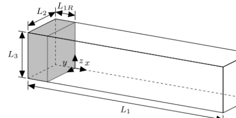
The classic lock-release setup is used as a test case for the model. This is a well-researched configuration with a range of data against which to validate results (Gladstone et al., 1998; Necker et al., 2002; Cantero et al., 2006; Espath et al., 2014). As defined in Fig. 2,L2=L3=2.0, which means that
h0=1.0, L1R=L3/2.0, and L1=19.0 which is slightly
longer than the final run-out length of the density current considered. The dimensionless parameters are set as Gr=5.0×10⁶, Sc=1.0,
us=0.02, Rp=20.0. (25)
As such, the experiment configuration is identical to that of Necker et al. (2002), with the exception of the addition of sediment erosion, and hence a requirement for the definition ofRp, which is defined to lie in the range ofRpfor which the
erosion algorithm outlined in Eq. (18) is valid, as detailed in Garcia and Parker (1991).
Boundary conditions for velocity are free-slip for all side walls, u1=0 atx= −1 andx=18,u2=0 at y=0, and
y=2, and no-slip at the top and bottom of the domain,
L1 L2
L3
L1R
x y z
Figure 2. Lock-release simulation domain configuration. The grey region indicates the volume of non-zero sediment concentration at t=0. The coordinate system defines the origin,x0,y0,z0
u=(0,0,0)T atz=0 andz=2. All velocity boundary con-ditions are applied weakly. Where a velocity component is not set with a Dirichlet condition, a zero Neumann boundary condition is applied. Note that the side wall boundary con-ditions vary from those of Necker et al. (2002). A free-slip boundary condition should give comparable results to the pe-riodic boundary conditions used in that work.
Boundary conditions for the sediment concentration field are as follows. The erosion boundary condition outlined in Eq. (17) is applied at the bottom surface, z=0. A zero Dirichlet boundary condition is prescribed atz=2 (the top surface of the tank). At all other boundaries (u+kus)·n
equals zero, hence zero Neumann boundary conditions are applied which enforce zero flux of sediment across these sur-faces.
The initial condition for the sediment concentration field in the three-dimensional simulation is similar to that suggested by Hartel et al. (1997) and Cantero et al. (2006). This initial condition is based upon the solution obtained from a purely diffusive problem. Hartel et al. (1997) argued that the prob-lem will be dominated by diffusion for very early stages of the simulation and hence this initial condition is justified as being the condition of the flow a short time period after the initial release. This initial condition includes a perturbation,
γ, in a similar way to the work by Cantero et al. (2006). A random perturbation of the initial condition is important to help promote the generation of three-dimensional structures in the flow. Necker et al. (2002) and Espath et al. (2014) use an alternative perturbation of the velocity field for the same purpose. The initial condition for the sediment concentration, including the perturbation, is as follows:
c=1
2− 1 2erf
np4
GrSc2[x−γ]o, (26)
with
γ=cos X
i
f (i, x, y, z)
!
where1x is chosen to be 0.2 and γ is constructed of four
sets of waves originating from the four corners of a plane aligned with the lock gate. Each set of waves contain 60 waves with random phases and random wavelengths rang-ing between 0.02 and∞. Waveihas amplitudef (i, x, y, z) at positionsx,y,z. The perturbation chosen covers a wide range of frequencies so as to not preferentially generate par-ticular wavelengths of oscillations. The mesh is adapted be-fore the first time step to produce a good mesh for this initial condition.
To use adaptivity several controlling parameters need to be defined. The fundamental parameters which define the mesh resolution in the simulation are the interpolation error bounds. The next section describes how values for these pa-rameters were chosen. The time between adapts also requires definitions, and it is necessary to ensure that there is adequate resolution in periods between adapts. Through experimenta-tion it was found that an adapt every five time steps kept the simulation stable towards the beginning of the simulation. At later stages in the simulation an adapt was required every two time steps. The high frequency of mesh adapts was re-quired to limit instabilities in the boundary layer which grow rapidly. Small instabilities that developed did not have any noticeable impact on the important outputs from the simula-tion. This is discussed further in the following sections. As mentioned in Sect. 2.3.1, metric advection is used to advect the metric, which defines the edge lengths required to meet the interpolation error bounds, forward in time. The metric is conservatively advected through five adapt intervals at each adapt.
4 Choosing appropriate interpolation error bounds It is possible to define an interpolation error bound for any of the functions in the simulation. In this simulation sediment concentration, velocity and pressure are solved for. It is com-mon practice to adapt to the velocity field for the purposes of resolving the velocity and pressure fields. Good resolution of the sediment concentration field is also required. Hence four interpolation error bounds require definition for the simula-tion – one for each velocity component, and another for the sediment concentration.
In order to select good values for these parameters a convergence analysis is required. Doing this with three-dimensional models would be prohibitively expensive and hence two-dimensional simulations are used to carry out this convergence analysis. The two-dimensional simulations are defined in the x–zplane. It has been well documented by Necker et al. (2002) and Cantero et al. (2007) that output from two-dimensional simulations of particle-laden density currents do not compare well with three-dimensional simu-lations. However, two-dimensional simulations are useful for the purpose of understanding the resolution requirements of simulations.
A measure of the quality of a mesh, in terms of the dy-namics computed within it, is required. The simulation is of a turbulent flow. Head speed, deposit profile, quantity of sus-pended sediment and deposition rates are all important out-puts from these simulations, but due to the turbulent nature of the flow, which is very sensitive to small changes in the mesh, it is very hard to show convergence of these quantities.
However, one important quantity does show convergence. This is the energy lost due to discretisation, and data transfer errors. DNS simulations resolve all length scales of motion. Convergence analysis will show that the discretisation errors are small enough that they have a negligible impact on the result and that the mesh resolution is fine enough to resolve all of the energy in the flow. The combination of upwind flux terms and slope limiting in the discretisation dissipates energy at scales that the mesh cannot resolve. Additionally, adapting the mesh requires a data transfer operation which will introduce some relatively small errors. By computing the energy budget in the simulation and how this varies over time a value for the energy lost due to discretisation, and data transfer errors,dcan be obtained. This quantity gives
us some indication of how well the scales of motion in the flow are being resolved. Importantly, this value converges as the mesh resolution increases and so gives us a good method of comparing the quality of different mesh configurations. Following the method of Winters et al. (1995), Necker et al. (2002) and Espath et al. (2014), equations for the rates of change of potential energy,Ep, and kinetic energy,Ek, in the
system can be derived as follows. The kinetic energy in the system is
Ek=
1 2 Z
|u|2d . (28)
To obtain the time derivative forEkcompute the dot product
of the momentum Eq. (15) withuand apply the chain rule to obtain
1 2
∂|u|2
∂t +
1 2uj
∂|u|2
∂xj = −ui
∂p ∂xi
−u3c+ui
∂τij ∂xj
. (29)
Integrating over the domain and integrating by parts, using the continuity Eq. (16) and the knowledge that there are no normal flow boundary conditions on all boundaries, i.e.
uini=0, an equation for the rate of change of Ek is
ob-tained:
∂Ek
∂t = −
Z
cu3d−
Z
τij
∂ui
∂xj
d . (30)
The potential energy in the system is
Ep=
Z
To obtain the time derivative for this term first multiply the equation for sediment concentration (Eq. 14) byx3:
∂c
∂tx3+x3(ui−uski) ∂c ∂xi
=x3
1 p
Sc2Gr ∂2c ∂xi∂xi
. (32)
Integrating over the domain, and by parts, using the chain rule and noting that all velocities normal to the wall are zero, an equation for the rate of change ofEpis obtained:
∂Ep
∂t =
Z
cu3d+us
Z
x3
∂c ∂x3
d
+ 1
p Sc2Gr
Z
0
x3
∂c ∂xi
nidσ−
Z
∂c ∂x3
d
. (33)
An equation for the transfer of energy fromEkandEpto and
from internal energy and heat, and also lost due to the settling of particles can be obtained by combining Eqs. (30) and (33). This equation will not hold for an under-resolved mesh. En-ergy dissipation that occurs at scales below the grid resolu-tion will be dissipated through applicaresolu-tion of slope limiting. An additional term, d, is therefore included to balance the
equation and represent the dissipation due to numerical er-rors which yields
∂ Ep+Ek
∂t = −−s−d, (34)
where
=
Z
τij
∂ui
∂xj
d , (35)
and
s=
1 p
Sc2Gr
Z
∂c ∂x3
d−
Z
0
x3
∂c ∂xinidσ
−us
Z
x3
∂c ∂x3
d . (36)
In order to compare overall mesh quality,dis integrated over
time to give the single quantity
ED= t
Z
0
|d(τ )|dτ . (37)
ED is computed for a set of two-dimensional simulations
forming a parameter sweep of values for the interpolation error bounds for the two components of velocity and sedi-ment concentration with values of 4×10⁻³, 4×10−2.5and 4×10⁻². This leads to a total of 27 simulations. The range of values used in the parameter sweep were determined from
104 105 106
10−1
mean number of elements ED
fixed adaptive
A0 A1 A2 A3
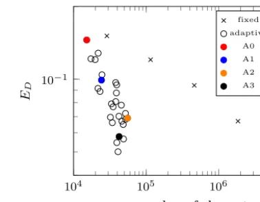
Figure 3. Time-integrated energy conservation error,ED, against
the mean number of elements for a range of two-dimensional simu-lations using fixed and adaptive meshes. Adaptive simusimu-lations rep-resent a parameter sweep of interpolation error bounds with val-ues 4×10⁻³, 4×10−2.5and 4×10⁻²for velocity and concentra-tion. Fixed meshes are on uniform triangular grids with edge lengths 5×10⁻², 2.5×10⁻², 1.25×10⁻²and 6.25×10⁻³. Four adaptive simulations are highlighted. The settings for these simulations are detailed in Table 1.
sensitivity analyses performed prior to this. For the pur-poses of comparing results against fixed mesh simulations the above quantity was also computed for a range of regu-lar, structured triangular mesh simulations with edge lengths 5×10⁻², 2.5×10⁻², 1.25×10⁻²and 6.25×10⁻³, result-ing in 2.88×10⁴, 1.15×10⁵, 4.6×10⁵and 1.84×10⁶ ele-ments respectively. The adaptive mesh simulations converge at a higher order than the fixed mesh simulations in relation to the mean number of elements,Ne, used in the simulation
(Fig. 3). The number of elements in adaptive mesh simula-tions,Ne, varies with time (Table 1). The difference between
the maximum and minimum number of elements increases superlinearly as the interpolation error bounds tighten. The number of elements in the domain is a function of the in-terpolation error bounds, the dynamics of the flow, which vary significantly with time, and also mesh resolution, cre-ating a non-linearity in this relationship, and also the bound set for the maximum element size. The largest relative dif-ference between the maximum and minimum number of ele-ments occurs in adaptive simulation A2 where the maximum is≈130 % of the mean, and the minimum is≈40 % of the mean. The distribution of element counts throughout a sim-ulation is skewed. An increase in the number of elements implies that element size has decreased. This in turn implies that the length of time steps has decreased, leading to more time steps being required at periods during which there are a large number of elements.
Table 1. Minimum, maximum and mean number of elements,Ne, and interpolation error bounds for sediment concentration,εc, thex
com-ponent of velocity,εu1, and theycomponent of velocity,εu2, for selected adaptive two-dimensional simulations from the interpolation error
bound parameter sweep.
id εc εu1 εu2 min(Ne) max(Ne) Ne
A0 4×10⁻² 4×10−2.0 4×10−2.0 12 924 15 000 14 017
A1 4×10−2.5 4×10−2.5 4×10−2.5 16 025 31 083 24 900
A2 4×10⁻³ 4×10−3.0 4×10−3.0 20 515 71 055 55 031
A3 4×10⁻³ 4×10−2.5 4×10−2.5 19 094 63 767 41 827
Integrating Eq. (38) over time,
Ep+Ek= t
Z
0
−(τ )−s(τ )−d(τ )dτ
= −E−Es−Ed. (38)
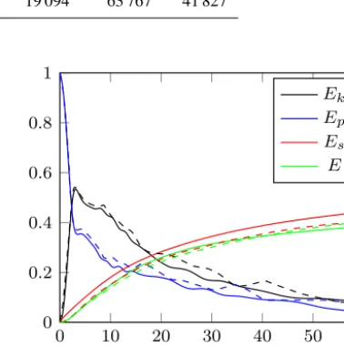
Figure 4 shows how the above quantities vary over the pe-riod of the simulation for adaptivity options A3, as detailed in Table 1. Values are compared against two-dimensional re-sults (Espath et al., 2014). There is very good agreement for
E, but there is a notable variation between the values forEs
in this work and that of Espath et al. (2014). This is because of the zero Dirichlet boundary condition for sediment con-centration at the top of the tank in this work whereas Espath et al. (2014) have a zero flux condition. At very early stages of the simulation the Dirichlet condition results in a flux of sediment through the top of the domain. The overall impact on the simulation is a loss of sediment mass of <1 % and a total energy loss of≈3 %. The zero flux condition is prefer-able but is not implemented in Fluidity for this discretisation. A future aim will be to implement this boundary condition. Generally there is good agreement for Ek andEp. In
two-dimensional simulations strong coherent vortices form that contain and transport large quantities of the suspended sed-iment. These vortices play an important role in the transfer of energy betweenEkandEp. Because of the chaotic nature
of the creation and propagation of the vortices, there will al-ways be variations in the values ofEk,Epand to some extent
Ebetween simulations.
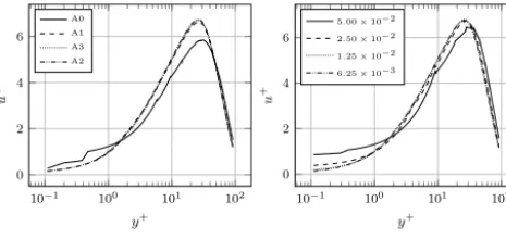
Another important aspect of the flow is the boundary layer at no-slip boundaries. This feature of the flow requires very small elements in the wall normal direction to resolve the boundary layer properly. Convergence on a solution is quickly obtained for the boundary layer using an adaptive mesh (Fig. 5). All but the most coarse adaptive simulation configurations have converged on to a solution. The fixed mesh configurations show a similar level of convergence for the two highest-resolution simulations. Anisotropic mesh adaptivity is particularly useful for resolving features such as boundary layers which require high resolution in one direc-tion compared to others.
Using the evidence outlined above, the chosen interpola-tion error bounds were those of adaptive simulainterpola-tion A3. This
0 10 20 30 40 50 60
0 0.2 0.4 0.6 0.8 1
t
Ek
Ep
Es
E
Figure 4. Energy budget evolution with time for simulation with adaptivity options A3 (solid lines —) compared against 2-D results from Espath et al. (2014) (dashed lines - - -). Values are normalised by the initial potential energy,ET.
simulation had a well-resolved boundary layer and good con-servation of energy. This simulation had interpolation error bounds of 4×10−2.5for both velocity components. An as-sumption is made that this error bound will also be suitable to use for the third velocity dimension in the three-dimensional simulation.
S. D. Parkinson et al.: Direct numerical simulations of particle-laden density with finite elements 1955
0 10 20 30 40 50 60
0 0.2 0.4 0.6 0.8 1
t
Ek
Ep
Es
E
Fig. 4: Energy budget evolution with time for simulation with adaptivity optionsA3(solid lines —) compared against 2-D results from Espath et al. (2014) (dashed lines - - - ). Values are normalised by the initial potential energy,ET.
10−1 100 101 102
0 2 4 6
y+
u
+
A0 A1 A3 A2
(a) Selected adaptive mesh simulations.
10−1 100 101 102
0 2 4 6
y+
u
+
5.00×10⁻²
2.50×10⁻²
1.25×10⁻²
6.25×10⁻³
(b) Fixed mesh simulations. Legend indicates element edge lengths.
Fig. 5: Wall normal velocity profile at the location of the nose of the gravity current att= 7.5for the fixed mesh simulations and selected adaptive simulations. Note thatAFigure 5. Wall normal velocity profile at the location of the nose2is a higher resolution simulation thanA3.
of the gravity current att=7.5 for the fixed mesh simulations and selected adaptive simulations. Note that A2 is a higher-resolution simulation than A3.
5 The benefits of using mesh adaptivity
In three dimensions, adaptivity is essential to compute this simulation using finite elements with Fluidity. A fixed, and regular tetrahedral grid would have required more than 1×
109 elements which would have led to an unachievable run time and unmanageable post-processing and visualisation demands. By using adaptivity the number of required el-ements has been reduced to a maximum of approximately 1×10⁷, at least a two order of magnitude reduction, making all aspects of the simulation manageable.
To resolve a comparable flow Espath et al. (2014) used
≈6×10⁷ degrees of freedom. A Fluidity simulation with O(109)discontinuous elements hasO(109)degrees of free-dom. The finite-difference method used by Espath et al. (2014) uses fewer degrees of freedom as it employs a high-order finite-difference discretisation which increases the ac-curacy of the solution.
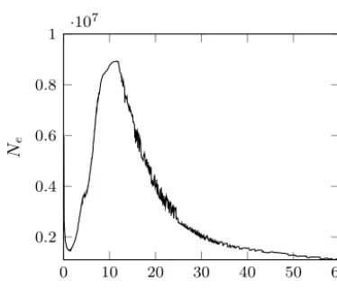
Figure 7 shows how the number of elements in the simu-lations varied over time. Throughout the simulation the num-ber of processor cores that were used was varied between 36 and 512 to keep the number of elements per core in the re-gion of 20 000. The initial drop in number of elements at the start of the simulation is due to the fact that conservative in-terpolation bounds were used to generate the mesh from the initial conditions. Following this initial drop, during early pe-riods of the simulation the flow is transitioning from a lam-inar to a turbulent flow. Throughout this period ubecomes more and more complex and hence the number of elements required to resolve the flow increase rapidly. The highest amount of elements required is at a t≈10 at which point the flow has developed into a fully three-dimensional, highly turbulent flow. Beyond this point the number of elements re-quired for the simulation steadily decreases as energy is dis-sipated from the flow. Additionally,cgradually diffuses such that the curvature of the field decreases and fewer elements are required to resolve the field. Note the drop in elements att≈25 of approximately 12.5 %. This coincides with the reduction in the number of time steps between adapts from
Fixed mesh Ne= 2.9×10⁴
Fixed mesh Ne= 1.8×10⁶
Adaptive mesh (A3) ¯ Ne= 4.1×10⁴
t= 4 t= 12
0 0.25 0.5 0.75 1
y
x
Figure 6. Heat map of sediment concentration att=4 andt=12 for the highest-resolution fixed mesh simulation, the adaptive sim-ulation with configuration A3, and a fixed mesh simsim-ulation with a similar number of elements to the adaptive simulation.
5 to 2 as mentioned in Sect. 3. A reduction in adapt interval means that the metric is not advected so far, and hence fewer elements are required. Also note the noise in the number of elements in the simulation. This is reduced by adapting more regularly and is due to the adapt routine responding to small instabilities in the boundary layer. Future work will look into removing these instabilities. This may require mesh adapts after every time step.
Figure 8 shows the adapted mesh over a subdomain in the region of the current head at two times,t=3.5 and t=4. The images are generated from the three-dimensional sim-ulation, and are taken from a plane aty=0. The cut plane is chosen to be at the edge of the domain as a good two-dimensional representation of the mesh can be obtained at boundaries where all element surfaces are parallel to one an-other. These images demonstrate how the mesh adapts to the concentration fieldc, and velocity field, u. The images also show how the mesh changes over a short period of the simulation. The change between t=3.5 and t=4 is dra-matic. Very few, if any elements, within this view are consis-tent. The images clearly display how anisotropic elements are generated along the density interface and the boundary layer where the curvature of the solution is highly anisotropic.
0 10 20 30 40 50 60 0.2
0.4 0.6 0.8
1 ·10
7
t Ne
Figure 7. Number of elements in the three-dimensional simulation as a function of time.
by a sharp interface in cat the front of the head. There is also high resolution around vortices and at the left-hand wall where there is a strong recirculation of the overlying fluid. The increase in resolution at the left-hand wall is present at botht=8 and att=20. The same increase in resolution is not present at the right-hand wall at either t=8 or t=20 (not shown in Fig. 9). This is because the fluid has more space to recirculate in front of the current than behind it in both cases such that the curvature of the velocity field, and thus the mesh resolution, is less. In theydirection the largest region of high resolution is in the gravity current body just behind the head of the current due to recirculating flow in this region and hence high curvature in candu2. The
dis-tribution of element sizes in this region varies rapidly due to the three-dimensional turbulent structure of the flow. There is a large difference in the resolution betweent=8 andt=20. Within the current the resolution has generally decreased by
t=20 but a significantly larger proportion of the domain is below the maximum element size. Generally, the elements appear to be smaller in thezdirection. This implies that the interpolation error bound may be proportionally tighter onu
in this direction, and could be reduced a little to bring the resolution in line with the other directions.
In Sect. 4 it was shown that an adaptive simulation with the interpolation error bounds used here compared well with the finest fixed mesh simulation (6.25×10⁻³). It is no surprise that, in the most computationally demanding regions of the flow, Fig. 9 shows that the smallest element edge lengths in the adaptive simulation match well with the fixed mesh edge length.
Adaptivity does of course come at a cost. The mean time required for a parallel adapt operation throughout this simu-lation, including mesh adaptation, data transfer, mesh parti-tioning and data migration, was 110 s. This can be compared to a mean time required to compute a time step in paral-lel of 67 s. Therefore, when adapting every five time steps, approximately 1/4 of the simulation time is spent adapting
c |u|
1.5 2 2.5 3 3.5 0
0.5 1
mesh
(a)t= 3.5
c |u|
1.5 2 2.5 3 3.5 0
0.5 1
mesh
(b)t= 4
Fig. 8: Images showing concentrationc, velocity magnitude|u|, and the adapted mesh att= 3.5(a) andt= 4(b) over the subdomain,3.5< x <3.75,z <1.25on ay-normal plane aty= 0.
∆x
∆y
0 2 4 6 8 10 12 0
2
∆z
(a)t= 8
∆x
∆y
0 2 4 6 8 10 12 0
2
∆z
(b)t= 20
0 2.5·10−2 5·10−2 7.5·10−2 0.1
z
x
Fig. 9: Heat map indicating the size of the elements inx,yandzacross a plane aty= 1for a subset of the domain (−1< x < 12) and timest= 8(left) andt= 20(right). Note that the domain extends tox= 18. The region12< x <18had no significant regions with element sizes smaller than0.1.
Figure 8. Images showing concentrationc, velocity magnitude|u|, and the adapted mesh att=3.5 (a) andt=4 (b) over the subdo-main, 3.5< x <3.75,z <1.25 on aynormal plane aty=0.
c |u|
1.5 2 2.5 3 3.5 0
0.5 1
mesh
(a)t= 3.5
c |u|
1.5 2 2.5 3 3.5 0
0.5 1
mesh
(b)t= 4
Fig. 8: Images showing concentrationc, velocity magnitude|u|, and the adapted mesh att= 3.5(a) andt= 4(b) over the subdomain,3.5< x <3.75,z <1.25on ay-normal plane aty= 0.
∆x
∆y
0 2 4 6 8 10 12 0
2
∆z
(a)t= 8
∆x
∆y
0 2 4 6 8 10 12 0
2
∆z
(b)t= 20
0 2.5·10−2 5·10−2 7.5·10−2 0.1
z
x
Fig. 9: Heat map indicating the size of the elements inx,yandzacross a plane aty= 1for a subset of the domain (−1< x < 12) and timest= 8(left) andt= 20(right). Note that the domain extends tox= 18. The region12< x <18had no significant regions with element sizes smaller thanFigure 9. Heat map indicating the size of the elements in0.1. x,yand
zacross a plane aty=1 for a subset of the domain (−1< x <12) and timest=8 (left) andt=20 (right). Note that the domain ex-tends tox=18. The region 12< x <18 had no significant regions with element sizes smaller than 0.1.
the mesh, or the run time is increased by 33 % compared to a fixed mesh simulation using the same number of elements. When adapting every two time steps approximately 1/2 of the simulation is spent in the adapt stage. The mesh optimi-sation algorithm used provides the most flexibility for mesh refinement, and hence will produce a highly optimised mesh, but it is potentially more expensive than other adaptivity al-gorithms. A high percentage of the total simulation time is spent in the adapt phase and hence it may be worth consid-ering cheaper alternatives based upon hierarchical refinement for future models. Regardless of this, the benefits of reducing the number of elements by two orders of magnitude far out-weigh the cost of adaptivity. The simulation required approx-imately 100 000 processor hours. Over 500 cores this equates to just under a week of run time. Assuming a linear increase in run time with number of elements, a fixed mesh simulation would have taken at least an order of magnitude longer and would have been nearly impossible to post-process.
0 2
4 6
8
Figure 10. Propagation of density interface over time. This figure shows a contour at a concentration 0.25 at times 0, 2, 8 and 14.
adapts requires a larger amount of elements to ensure that there is adequate resolution throughout the period between adapts. This will increase the number of processing hours re-quired to solve the problem. However, with more elements, the problem can be split amongst more cores whilst keep-ing the minimum number of elements per core constant. The time to completion is then likely to reduce as fewer adapt operations are required. This parameter can be varied depen-dent upon what is important to the scientist. Size of output, time to completion, the cost of processor time, and the size of available computers must all be taken in to account. Another adaptive simulation with similar properties, but slightly var-ied parameters, could require significantly more, or less total processing hours.
6 Results
Figure 10 shows how the density current propagates along the tank in three dimensions. The perturbation in the ini-tial condition for the concentration field is shown in the im-age relating tot=0. This initial condition creates the initial three-dimensional instabilities required to generate a realis-tic density current. Byt=8 this flow is fully turbulent and three-dimensional. This is in agreement with other models (Necker et al., 2002; Espath et al., 2014). The well-known structures of lobes and clefts are present at the front of the density current from this point onward.
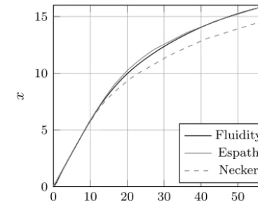
Figure 11 shows how the head position varies with time throughout the simulation. This is computed as the maximum
x value, averaged across the width of the domain, obtained from a sediment concentration contour atc=0.01. Lines are plotted showing the agreement with other models. The re-sults compare well with Espath et al. (2014), whose model predicted a head position slightly in front of the model by Necker et al. (2002). Espath et al. (2014) noted the impor-tance of the initial condition to the development of the flow. The initial conditions used in this work are slightly different to those of Espath et al. (2014) and Necker et al. (2002) and hence complete agreement is not expected.
0 10 20 30 40 50 60
0 5 10 15
t
x
Fluidity Espath Necker
Figure 11. Position of density current head against simula-tion time for the Fluidity simulasimula-tion and the simulasimula-tions of Necker et al. (2002) and Espath et al. (2014).
Figure 12 shows the spatially integrated deposition rates over the course of the simulation. Again the deposition rate shows good agreement with other published values. As noted by Necker et al. (2002), the deposition rate increases at a rate proportional to t0.5 until approximately t=14, at which point there is a sharp change and the deposition rate begins to drop rapidly at a rate proportional tot−2.5. A key difference between the results from this work and those of the other models is the presence of erosion in this simulation. The de-position rates from this simulation are higher than those of Necker et al. (2002) and Espath et al. (2014). Noting that the vertical fluid velocities are small near the bed due to the no-slip boundary condition, and that eroded sediment will be settling, the majority of eroded sediment will almost imme-diately be deposited, and will never be fully entrained back into the flow. This will lead to an increased deposition rate compared to a simulation without erosion. By making the as-sumption that all eroded sediment is immediately deposited, a modified deposit rate can be calculated for the Fluidity simulation with the effect of erosion removed. As shown in Fig. 10, this modified deposition rate shows much better agreement with the results of both Necker et al. (2002) and Espath et al. (2014), leading to the conclusion that it is the inclusion of erosion in the simulation that led to the higher deposition rate.
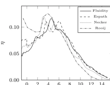
An important diagnostic for applications is the final de-posit profile from a particle-laden density current. Fig-ure 13 shows the span-wise averaged deposit profile from the three-dimensional Fluidity simulation compared against those of previous modellers and also from the experiments of De Rooij and Dalziel (2001). A good match is observed in the peak deposit height ofη≈0.12 atx1≈4 between all of
the models and the experimental results.
100 101
10−3
10−2 10−1
t0.5
t−2.5
t
d
R
R
η
d
x
d
y
d
t
Fluidity (F1) Fluidity (F2)
Espath Necker
Figure 12. Deposition rates for the three-dimensional simulation. Deposition rates from Fluidity (F1), Fluidity with a modified de-position rate where the erosion rate has been removed (F2), Espath et al. (2014), and Necker et al. (2002).
0 2 4 6 8 10 12 14 16
0.00 0.05 0.10
x
η
Fluidity Espath Necker Rooij
Figure 13. Span-wise averaged deposit profile from the three-dimensional simulation att=60. Comparisons are made against numerical results of Necker et al. (2002) and Espath et al. (2014) and experimental results of De Rooij and Dalziel (2001).
this is unclear and explanations can only be speculative. One potential cause may be that the sediment in the experimen-tal setup had already begun to settle before the lock gate was released. This may also help to explain the slightly shorter run-out distance resulting from a reduced initial potential en-ergy. Alternatively, there may be processes occurring in the laboratory that are not accurately captured by the computa-tional models.
The results from Fluidity are further from the measured results than the other models in this region. The inclusion of an erosion algorithm is the likely cause of this. The ex-perimental measurements show larger deposits than all of the models upstream, and smaller deposits downstream. Ero-sional processes will predominately decrease upstream de-posits and increase downstream dede-posits, and hence would increase this discrepancy if applied to any of the models. In addition to this, the erosion algorithm is not configured cor-rectly to match the De Rooij and Dalziel (2001) experiment:
Rp≈1 for the De Rooij and Dalziel (2001) experiment, in
comparison toRp≈20 in the Fluidity simulation. This will
result in significantly more erosion in the simulation than is likely to have occurred in the experiment.
7 Conclusions
This paper presents validation of a novel three-dimensional finite-element model for simulating particle-laden density currents. The model is validated by assessing the con-vergence of key variables in two-dimensional simulations and by comparison with results from previous DNS three-dimensional simulations by Necker et al. (2002) and Espath et al. (2014). It has been shown that by using adaptive mesh-ing the number of required elements in these simulations can be reduced by between one and two orders of magnitude. This makes DNS modelling of particle-laden density currents at moderate Grashof numbers an achievable goal using finite elements.
In addition, simulations within complex domains can be achieved fairly trivially using the flexibility afforded by un-structured finite elements. Future work will study flow of tur-bidity currents along circular channels and across breaks in slope, and will help answer outstanding questions about the dynamics of flows in these situations. Using mesh adaptiv-ity also makes modelling in very large domains achievable. Large regions of the domain where very little is happening come at very little cost. This will enable modelling turbidity currents in deep water where the dynamics are not dominated by the bore created by the overlying fluid. It may also allow for simulations of turbidity current along sinuous channels with over-spilling as well as numerous other similar scenar-ios.
The cost of these simulations is still very high. It may be possible to further reduce the cost of these simulations, whilst retaining important three-dimensional dynamics, using large eddy simulation (LES). Future work will focus on implemen-tation and testing of LES for this simulation with the aim of reducing the simulation cost.
Acknowledgements. The authors would like to acknowledge the work of the Fluidity development team for their prior development work and assistance in developments required for this work, especially G. Gorman for his help regarding three-dimensional adaptivity. The authors would also like to acknowledge the assistance provided by the HPC team at Imperial College London, especially S. Burbidge who provided prompt assistance and useful guidance. The lead author would like to thank S. Mouradian, F. Mithaler, D. Robinson and S. Funke for many stimulating discussions related to this work. Finally, the authors would like to thank the reviewers and the editor for their comments which have led to a much improved paper.
References
Akiyama, J. and Stefan, H.: Turbidity current with erosion and de-position, J. Hydraul. Eng.-ASCE, 111, 1473–1496, 1985. Alavian, V., Jirka, G., Denton, R., Johnson, M., Stefan, H.,
and Members, A.: Density currents entering lakes and reservoirs, J. Hydraul. Eng.-ASCE, 118, 1464–1489, doi:10.1061/(ASCE)0733-9429(1992)118:11(1464), 1992. Bassi, F. and Rebay, S.: A high-order accurate discontinuous finite
element method for the numerical solution of the compressible Navier–Stokes equations, J. Comput. Phys., 131, 267–279, 1997. Best, J., Kotaschuk, R., Peakall, J., Villard, P., and Franklin, M.: Whole flow field dynamics and velocity pulsing within natural sediment-laden underflows, Geology, 33, 765–768, doi:10.1130/G21516.1, 2005.
Blanchette, F., Strauss, M., Meiburg, E., Kneller, B., and Glin-sky, M.: High-resolution numerical simulations of resuspend-ing gravity currents: conditions for self-sustainment, J. Geophys. Res., 110, C12022, doi:10.1029/2005JC002927, 2005.
Boman, E. G., Catalyurek, U. V., Chevalier, C., and Devine, K. D.: The Zoltan and Isorropia parallel toolkits for combinatorial sci-entific computing: partitioning, ordering, and colorin, Scisci-entific Programming, 20, 129–150, 2012.
Bombardelli, F., Cantero, M., Buscaglia, G., and Garcia, M.: Comparative study of convergence of CFD commercial codes when simulating dense underflows, Mecánica Computacional, 23, 1187–1199, 2004.
Bonnecaze, R., Huppert, H., and Lister, J.: Particle-driven gravity currents, J. Fluid Mech., 250, 339–339, 1993.
Cantero, M., Balachandar, S., Garcia, M., and Ferry, J.: Direct nu-merical simulations of planar and cylindrical density currents, J. App. Mech., 73, 923–930, doi:10.1115/1.2173671, 2006. Cantero, M., Lee, J., Balachandar, S., and Garcia, M.: On the
front velocity of gravity currents, J. Fluid Mech., 586, 1–39, doi:10.1017/S0022112007005769, 2007.
Cantero, M. I., Garcia, M. H., and Balachandar, S.: Effect of particle inertia on the dynamics of depositional par-ticulate density currents, Comput. Geosci., 34, 1307–1318, doi:10.1016/j.cageo.2008.02.002, 2008.
Chen, L., Sun, P., and Xu, J.: Optimal anisotropic meshes for min-imizing interpolation errors in Lp-norm, Math. Comput., 76, 179–204, 2007.
Ciarlet, P. G.: Basic error estimates for elliptic problems, in: Hand-book of Numerical Analysis, 2, 17–351, 1991.
Cockburn, B. and Shu, C.-W.: Runge–Kutta discontinuous Galerkin methods for convection-dominated problems, J. Sci. Comput., 16, 173–261, 2001.
Cotter, C. J., Ham, D. A., Pain, C. C., and Reich, S.: LBB stability of a mixed Galerkin finite element pair for fluid flow simulations, J. Comput. Phys., 228, 336–348, doi:10.1016/j.jcp.2008.09.014, 2009.
Curran, K., Hill, P., and Milligan, T.: The role of particle aggrega-tion in size-dependent deposiaggrega-tion of drill mud, Cont. Shelf Res., 22, 405–416, doi:10.1016/S0278-4343(01)00082-6, 2002. Davis, R. H. and Hassen, M. A.: Spreading of the interface at the
top of a slightly polydisperse sedimenting suspension, J. Fluid Mech., 196, 107–134, 1988.
De Rooij, F. and Dalziel, S. B.: Particulate Gravity Currents, Vol. 31 of Special Publication International Association of Sedimentol-ogists, chap. Time- and Space-Resolved Measurements of
De-position under Turbidity Currents, edited by: McCaffrey, W., Kneller, B. C., and Peakall, J., 207–215, Blackwell Publishing Ltd., doi:10.1002/9781444304275.ch15, 2001.
Donea, J. and Huerta, A.: Finite Element Methods for Flow Prob-lems, John Wiley & Sons, Ltd, doi:10.1002/0470013826.fmatter, 2005.
Espath, L., Pinto, L., Laizet, S., and Silvestrini, J.: Two-and three-dimensional direct numerical simulation of particle-laden gravity currents, Comput. Geosci., 63, 9–16, doi:10.1016/j.cageo.2013.10.006, 2014.
Farrell, P. and Maddison, J.: Conservative interpolation between volume meshes by local Galerkin projection, Comput. Method. Appl. M., 200, 89–100, 2011.
Farrell, P., Piggott, M., Pain, C., Gorman, G., and Wilson, C.: Con-servative interpolation between unstructured meshes via super-mesh construction, Comput. Method. Appl. M., 198, 2632–2642, 2009.
Fortin, M.: Estimation a posteriori et adaptation de maillages, Revue Européenne des Éléments Finis, Rev. Eur. Élém. Finis, 9, 369– 504, 2000.
Frey, P.-J. and Alauzet, F.: Anisotropic mesh adaptation for CFD computations, Comp. Method. Appl. M., 194, 5068–5082, 2005. Fukushima, Y., Parker, G., and Pantin, H.: Prediction of ignitive tur-bidity currents in Scripps Submarine Canyon, Mar. Geol., 67, 55–81, 1985.
Garcia, M. and Parker, G.: Entrainment of bed sediment into sus-pension, J. Hydraul. Eng.-ASCE, 117, 414–435, 1991.
Georgoulas, A., Angelidis, P., Panagiotidis, T., and Kotsovinos, N.: 3D numerical modelling of turbidity currents, Environ. Fluid Mech., 10, 603–635, doi:10.1007/s10652-010-9182-z, 2010. Gladstone, C., Phillips, J., and Sparks, R.: Experiments on
bidis-perse, constant-volume gravity currents: propagation and sedi-ment deposition, Sedisedi-mentology, 45, 833–843, 1998.
Hallworth, M. and Huppert, H.: Abrupt transitions in high-concentration, particle-driven gravity currents, Phys. Fluids, 10, 1083–1087, 1998.
Harris, T., Hogg, A., and Huppert, H.: Polydisperse particle-driven gravity currents, J. Fluid Mech., 472, 333–371, doi:10.1017/S0022112002002379, 2002.
Hartel, C., Kleiser, L., Michaud, M., and Stein, C.: A direct numer-ical simulation approach to the study of intrusion fronts, J. Eng. Math., 32, 103–120, 1997.
Hartel, C., Meiburg, E., and Necker, F.: Analysis and direct numer-ical simulation of the flow at a gravity-current head. Part 1. Flow topology and front speed for slip and no-slip boundaries, J. Fluid Mech., 418, 189–212, 2000.
Heezen, B. C. and Ewing, W. M.: Turbidity currents and submarine slumps, and the 1929 Grand Banks [Newfoundland] earthquake, Am. J. Sci., 250, 849–873, 1952.
Hiester, H., Piggott, M., and Allison, P.: The impact of mesh adaptivity on the gravity current front speed in a two-dimensional lock-exchange, Ocean Model., 38, 1–21, doi:10.1016/j.ocemod.2011.01.003, 2011.
Hiester, H., Piggott, M., Farrell, P., and Allison, P.: Assessment of spurious mixing in adaptive mesh simulations of the two-dimensional lock-exchange, Ocean Model., 73, 30–44, 2014. Huang, H., Imran, J., and Pirmez, C.: Numerical model of