Gene masking - a technique to improve accuracy for cancer classification with high dimensionality in microarray data

R E S E A R C H

Open Access

Gene masking - a technique to improve

accuracy for cancer classification with high

dimensionality in microarray data

Harsh Saini

, Sunil Pranit Lal

, Vimal Vikash Naidu

, Vincel Wince Pickering

, Gurmeet Singh

,

Tatsuhiko Tsunoda

and Alok Sharma

From15th International Conference On Bioinformatics (INCOB 2016) Queenstown, Singapore. 21-23 September 2016

Abstract

Background: High dimensional feature space generally degrades classification in several applications. In this paper, we propose a strategy called gene masking, in which non-contributing dimensions are heuristically removed from the data to improve classification accuracy.

Methods: Gene masking is implemented via a binary encoded genetic algorithm that can be integrated seamlessly with classifiers during the training phase of classification to perform feature selection. It can also be used to

discriminate between features that contribute most to the classification, thereby, allowing researchers to isolate features that may have special significance.

Results: This technique was applied on publicly available datasets whereby it substantially reduced the number of features used for classification while maintaining high accuracies.

Conclusion: The proposed technique can be extremely useful in feature selection as it heuristically removes non-contributing features to improve the performance of classifiers.

Background

Traditionally, clinical methods are employed to detect cancers such as ultrasonography, X-Ray, Computed Tomography (CT) and Magnetic Resonance Imaging (MRI) [1]. However, many cancers cannot be distin-guished easily using traditional approaches. An alternative approach to improve detection is to use analyze microar-ray gene profiles. In microarmicroar-ray gene profiles, mRNA samples are used to measure the expression level of genes, which can be in the magnitude of thousands. This in turn makes detection and classification of difficult due to the high dimensionality in data [2], therefore, there is a need for computation methods to help improve the classification of cancers using microarray gene profiles.

*Correspondence: [email protected]; [email protected]

1_{The University of the South Pacific, Laucala Bay, Suva, Fiji}

3_{RIKEN Center for Integrative Medical Sciences, 230-0045 Yokohama, Japan}

Full list of author information is available at the end of the article

Generally, computational methods are used to remove non-contributing and noisy dimensions from data while simultaneously trying to maintain a high classification rate [3]. Additionally, class imbalance is an important consid-eration in classification of biomedical data, and there are techniques [4] which incorporate class distribution within the classification algorithm. Our approach is different in that we separate the classification from data preprocessing where we assume class imbalance is to be handled.

Feature selection and extraction is a well researched topic in biomedical fields, especially in the areas concern-ing microarray data [5–7]. Several methods have been discussed relating to feature selection for microarray data [6, 8–17] and they can be broadly categorized into two groups, filter based methods and wrapper based meth-ods. In filter based methods, genes are selected prior to training the classification model whereas wrapper based methods involve gene selection within the classification process [5, 18, 19].

The importance of selecting features from gene subsets or groups has recently become popular topic in microar-ray research [7, 20]. For instance, top-r feature selection proposed by Sharma et. al [20] does provide very good results based on a small subset of genes, however, it should be noted that it has a few drawbacks. Firstly, it is quite computationally expensive, requiring a total number of search combinations betweenh+1C2×(d/h)and(2h −

1)×(d/h), where his the block size and d is the total number of dimensions [20]. Additionally, initial parameter selection is crucial and it greatly affects the final results. Top-r is sensitive to the selection of block size and num-ber of resulting blocks. Selecting ideal value ofhcould be a tricky task and final results are dependent on this value [20]. Lastly, it should be noted that top-r does not fully consider the interaction among features but only amongst the top-r features from each block [5].

In this paper, we consider the classification of the small round blue cell tumor (SRBCT) [21] dataset which has been categorized into 4 types of cancers and has 2308 gene expressions. Khan et al. [1], Tibshirani et al. [21] and Kumar et al. [22] have previously worked on this dataset whereby they have all reported 100% classification accu-racies with 96, 43 and 13 genes respectively. While Khan et al. [1] and Tibshirani et al. [21] use the fully-fledged dataset with 2308 genes to perform analysis, Kumar et al. [22] begin their analysis from a reduced set of 96 genes (from Khan et al. [1] findings) to obtain results. Kumar et al. [22] do not use all 2308 genes due to the com-putational complexity of their approach. Our motivation in this paper is to build upon the approach proposed by Kumar et al. [22] and propose a new method that does not suffer from similar limitations. In the proposed method, we propose a wrapper based method where we commence with the entire feature set from the microar-ray data without any prior need of feature selection and achieve high classification accuracy with as few features as possible.

Furthermore we validate our approach using the mixed-lineage leukemia (MLL) [23] and lung cancer (LC) [24] datasets. MLL dataset comprises of 3 classes, with each sample containing 12,582 gene expressions. Lastly, LC dataset contains 2 cancer types and each sample com-prises of 12,533 gene expressions. We applied gene mask-ing with nearest shrunken centroid classifier to signifi-cantly reduce the number of dimensions for the datasets while maintaining 100% accuracies during classification.

Methods

Gene masking has been derived from genetic algorithm, whereby genetic algorithm is used to search for an opti-mal gene mask that provides the greatest performance gains while removing the most number of features for the selected classification algorithm. For this study, Nearest

CentroidandNearest Shrunken Centroidclassifiers were used for classification.

Genetic algorithm

The genetic algorithm (GA) is a heuristic search based algorithm inspired by Darwin’s theory of natural selection. It was first introduced by Holland and it simulates nat-ural processes of evolution, namely selection, crossover and mutation. GA is a competitive search algorithm where evolution of individuals is directed mainly by the princi-ple of “survival of the fittest”. Fitness of an individual is determined by a fitness function and individuals with a higher fitness have a greater bias for contributing to the next generation than their less fit counterparts [25]. More details on GA processes and functions are described in latter sections.

Nearest centroid classifier

Nearest Centroid Classifier (NCC) is a basic prototype classifier that creates centroids (which is the mean for a particular class) to create a classification model. Samples closest to a centroid is assigned a label of that particular class [21].

In NCC, we compute the class centroid by finding the mean of every feature per class:

¯

x_ik= jCk

xij nk

(1)

where xij is the value at the ith feature of the jth sam-ple,kdenotes the class under consideration andnk is the number of samples in class k. Once the class centroids can calculated, we can predict the classkˆfor an unknown samplexˆusing:

ˆ

k=arg min_kK||¯x_k− ˆx|| (2)

Nearest shrunken centroid classifier

Nearest Shrunken Centroid Classifier (NSCC) [21], is a simple modification of NCC that uses “de-noised” ver-sions of the centroids. Features that are noisy and have little variation from the overall mean are removed dur-ing shrinkage. The amount of shrinkage is determined by a constant, where a larger value ofremoves a larger number of features. Therefore, it can be stated that this classifier has an “in-built” feature selection mechanism.

In order to perform the shrinkage, firstly, we compute the distance of every feature, dik, from the overall cen-troid after standardizing by standard deviation of features within a class. In Eq. 3,xij is the value at the ith feature of thejthsample,Kis is the total number of classes andk denotes the class under consideration. The centroid values for featureiin classkisx¯ik =jCk

xij

nk, whereCkdenotes

centroid value at theith_{feature isx¯}

i=nj=1

xij

n. Also,mkis defined asm2_k= _n1

k−

1

nands2i = n−1K

k

jCk(xij−¯xik)

2_,

which is the pooled within-class variance for featurei.s0

was chosen to be the median value ofsi.

dik = ¯ xik− ¯xi mk×(si+s0)

(3)

Once the distances are computed, we perform the actual shrinkage where everyd_ik is reduced by an amountin absolute value and is set to zero if its absolute value is less than zero. In Eq. 4,+means we only consider the positive part (t+=tift≥0 otherwise zero).

d_ik =sign(dik)(|dik| −)+ (4)

In the above equation, d_ik defines the shrunken dis-tances. By usingas a soft threshold, we are effectively removing features that have little or no variation from the overall centroids. In order to obtain the shrunken class centroids,x¯_ik, we can rewrite Eq. 3 and substitutedikwith their shrunken representationsd_ik(Eq. 5) after which we can predict unknown samples as per Eq. 2.

¯

x_ik = ¯xi+mk(si+s0)dik (5)

Gene masking

Gene masking is a technique that incorporates evolu-tionary techniques to reduce the dimensionality of data within the training phase of the classification model. The basic premise of this technique is to heuristically remove non-contributing features in data while training the clas-sifier. The amount of contribution by a feature is deter-mined by its impact on classification accuracy, whereby non-contribution is attributed to features whose removal and/or existence has minimal effect on classification accu-racy. By reducing the dimensionality of data, gene mask-ing helps improve classifier performance and reduces the computational complexity of the problem. Moreover, it can be used as a feature isolation technique that allows for the identification of features which contribute the most towards classification.

Overview

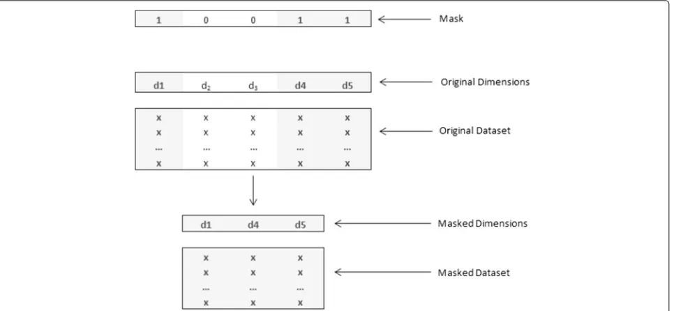
Gene masking, essentially, is a binary encoded genetic algorithm that generates a template used to represent a chromosome, referred to as a mask, while the individual bits at different indices in the chromosome are annotated as genes. This mask can be visualized as a string of binary digits with length equal to the number of features in data. Each binary digit at a particular index (or a gene in terms of the mask) signifies the presence or absence of the cor-responding feature in data. For instance, a problem with five features can represented by a feature vector[f1 f2 f3 f4 f5]and a possible gene mask can be[1 0 0 1 1]. This mask indicates that featuresf2andf3are to be removed from the

data and the classification model has to be created using a feature vector comprising of[f1 f4 f5], thus, effectively reducing the dimensionality of data. This process has been depicted in Fig. 1.

In gene masking, the GA processes are unmodified and it goes through its basic set of genetic operations. For each generation, fitness is calculated for every mask in the pop-ulation. These masks are then exposed to the three GA operators; selection, crossover and mutation. Finally, the best performing mask is chosen after the generation limit is reached in GA.

In essence, the basic purpose of GA in gene masking can be viewed as heuristically searching for the optimal gene mask that reduces the most features for a particular prob-lem while maintaining high classification accuracy. The holistic approach taken when applying gene masking is shown in Fig. 2.

Process details

In order to determine the fitness of each mask, a clas-sifier model is created using the masked dataset and its classification accuracy is evaluated usingk-fold cross val-idation. The masked dataset is divided intok number of folds and a model is iteratively built usingk-1folds and while thekthfold is isolated for model evaluation, yield-ing a set containyield-ingkclassification accuracy values (one for each fold). Then, the fitness of a mask is computed based on its impact on classification accuracy while also considering the effective reduction in dimensionality. The details of fitness evaluation for gene masking is high-lighted in Fig. 3, which describes intricacies between the classification algorithm and the masking process.

Upon fitness evaluation, GA goes through its orthodox set of operators, namely selection, crossover and muta-tion. Selection has been performed using roulette wheel selection, which is biased towards individuals with higher fitness. Crossover is accomplished by performing a ran-dom one-point binary crossover to swap the genes and mutation is performed by negating gene values at random locations. However, to preserve the highest performing chromosome between generations, elite selection is used to ensure that a mask with the highest fitness is passed to the next generation unmodified by GA operators.

Fig. 1Illustration of gene masking on the original dataset to produce a masked dataset

Gene mask

Fitness

Compute average k-fold cross validation accuracy of the gene mask

Fig. 2Flowchart depicting the relation of Genetic Algorithm and Classifier in gene masking where the best chromosome represents the best gene mask discovered

give higher fitness values to masks with greater number of genes eliminated.

Fitness=(Accuracy×α)+(1−α)×Genes eliminated Total genes

(6)

This process of performing fitness evaluations and applying genetic operators continues until the number of generations specified during the initial parameter con-figuration is reached. The best chromosome discovered during the evolution of the population is selected. This chromosome represents the gene mask that yielded the highest fitness value during training. The best evolved gene mask is subsequently used for masking the test dataset during the testing phase.

Experiment and discussion

Primarily, we had considered the SRBCT dataset for gene masking. The following sections provide details on the data, and the experiment and its results.

Dataset

Fig. 3Illustration of fitness evaluation with gene masking. Cross validation is performed using a classifier and the average accuracy is used for fitness calculation

tumors (EWS). The dataset comprises of 63 training sam-ples and 25 test samsam-ples, each of which contains 2308 gene expressions from cDNA microarrays [1, 21]. Of the 25 test samples, 5 samples are not SRBCTs, which were discarded for the purpose of this study since correspond-ing non-SRBCT samples were not present in the train-ing set. Classification by microarrays is a difficult task since the number of features (genes) are relatively large whereas the number of samples are relatively small and it is also important to identify genes that contribute most to classification [1, 21].

Results

GA, and subsequently, gene masking, is stochastic by nature. During our experiment, multiple experiments with the same parameter combinations were executed while tuning GA parameters to get a consolidated view on the performance of gene masks with a particular combi-nation of parameters.

As stated previously, gene masking is implemented by applying a mask to select a subset of features from data.

GA is used to heuristically create masks (represented as a chromosome within GA) and evaluate their rela-tive fitness. The parameters for GA were determined by empirical testing, whereby the population size was fixed to 105 and the chromosome length set to 2308 (the number of gene expressions in SRBCT dataset), and the best performing rates for crossover and mutation were determined to be 0.85 and 0.1 respectively. These initial parameter configurations were determined by experimen-tally evaluating the performance of GA with multiple experimental runs (around 10 runs for each combina-tion of parameters) to produce a baseline from which the best parameter configurations were selected. The initial parameter configurations of GA are shown in Table 1. These simulations were conducted withk-fold cross vali-dation fork = 5. The actual parameter tuning and selection procedure has been described in an algorithmic form in Table 2.

Table 1Genetic algorithm parameters

Parameter Value

GA type Binary

Population size 105

Chromosome length 2308

No. of generations 50000

Selection function Roulette wheel

Crossover rate 0.85

Mutation rate 0.10

Elite conservation Yes, num_elite=1

with 100% classification accuracy, however, there was only about 28% reduction in genes (about 650 genes) from the original microarray data. This may be attributed to the fact that NCC is a very basic classifier. Additionally, it can be noted that with NCC, having a lower value for α(signifying a greater preference towards dimensionality reduction) yielded better results withα=0.3, giving 100% training and test accuracies.

The experiment was repeated by replacing NCC with NSCC whereby the results considerably improved. There was significant reduction in dimensionality while main-taining high classification accuracy. The best results with NSCC were shown with a solution comprising of 13 genes with 100% training and test accuracies. However, it must be stated that with NSCC, gene masking was performed on a “shrunken” dataset with about 70-120 genes depend-ing on the value of . The optimal range values for that produced the best overall performance were in the

Table 2Parameter tuning and selection method used in this study

Parameter tuning and selection

LetSbe the set of training samples

LetCRbe the crossover rate andMRbe the mutation rate

Letkbe the number of cross validation folds, wherek= 5 is fixed

Letαbe theAccuracy to Elimination Ratio

Define the GA parameters apart fromCRandMRas those highlighted in Table 1

Define_αto belong to the set (0, 0.1, 0.2, . . . , 0.9, 1]

DefineCRto belong to the set (0.5, 0.55, 0.6, . . . , 0.95, 1]

DefineMRto belong to the set [0, 0.05, 0.1, . . . , 0.45, 0.5)

For each combination of {α,CR,MR}:

- Performk-fold cross validation using the classifier and gene masking on the set of samplesS

- Report the results obtained by the best performinggene mask

- Repeat for 10 iterations

Select the best performing combination of {_α,CR,MR} for testing and reporting

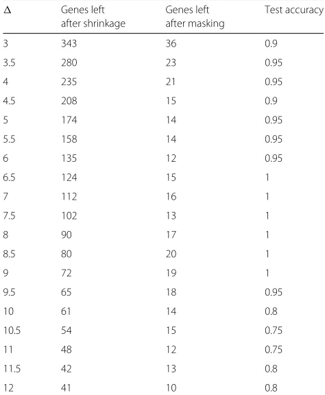
interval of (6, 9] with steps of 0.5. Additionally, the optimal value that was observed forαwasα=0.9signifying that a greater bias towards accuracy yielded better results with NSCC. The performance of gene masking with NSCC for varying values ofis shown in Table 3. The training accu-racies for each of the reported samples in Table 3 was 100%. Additionally, a comparison of performance of gene masking with NCC and NSCC is highlighted in Table 4.

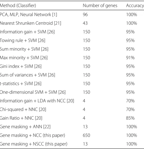
NSCC removes features only on the basis of their mag-nitude of deviation of the classful means from the overall mean and, therefore, the interdependencies between fea-tures are not considered. Tibshirani et al. [21] used NSCC with the SRBCT dataset and identified 43 genes that lead to 100% classification accuracy. However, with gene mask-ing, similar classification accuracy was achieved with only 13 genes. This can be attributed to the fact that gene masking eliminates genes based on their impact on clas-sification, identifying major interdependencies between features and ensuring their survival during the evolu-tion of gene masks. A comparison of results with similar techniques has been illustrated in Table 5.

In NSCC, if the amount of shrinkage is kept relatively low (a lower value for, which leaves more features in the dataset), gene masking is able to evaluate interdependen-cies between the remaining features. With the proposed technique, genes that were previously eliminated solely

Table 3Gene masking and NSCC performance on SRBCT test set with different values forwithα= 0.9

Genes left Genes left Test accuracy

after shrinkage after masking

3 343 36 0.9

3.5 280 23 0.95

4 235 21 0.95

4.5 208 15 0.9

5 174 14 0.95

5.5 158 14 0.95

6 135 12 0.95

6.5 124 15 1

7 112 16 1

7.5 102 13 1

8 90 17 1

8.5 80 20 1

9 72 19 1

9.5 65 18 0.95

10 61 14 0.8

10.5 54 15 0.75

11 48 12 0.75

11.5 42 13 0.8

Table 4Comparison of performance of NCC and NSCC with gene masking

NCC NSCC

Number of genes remaining 1637 13

Training accuracy 100% 100%

Test accuracy 100% 100%

on the value of are kept. Gene masking commences with around 100-120 genes, which are systematically eval-uated and eliminated based on the gene masks produced by GA. Eventually, gene masking yields a solution with only 13 genes and as per the results shown in Table 6, it can be seen that only 6 of the genes discovered in the best solution of 13 genes belong to the 43 genes identified by Tibshirani et al. [21]. Also, it can be seen that majority of the genes identified by gene masking are also present in the 96 genes identified by Khan et al. [1]. Conversely, it can also be seen that this approach yields different results to those achieved by Kumar et al. [22], by noting the lack of any significant overlap between the identified genes.

Furthermore, due to the stochastic nature of gene mask-ing, the gene masks that produce 100% accuracies do not tend to select the same combination of genes. Therefore, we have also identified and reported the relative occur-rence of these genes (in Table 6) during various iterations where solutions that gave 100% accuracy with 15 genes or less were observed.

Table 5Comparison of performance of similar techniques

Method (Classifier) Number of genes Accuracy

PCA, MLP, Neural Network [1] 96 100%

Nearest Shrunken Centroid [21] 43 100%

Information gain + SVM [26] 150 95%

Towing rule + SVM [26] 150 95%

Sum minority + SVM [26] 150 95%

Max minority + SVM [26] 150 91%

Gini index + SVM [26] 150 95%

Sum of variances + SVM [26] 150 95%

t-statistics + SVM [26] 150 95%

One-dimensional SVM + SVM [26] 150 95%

Information gain + LDA with NCC [20] 4 70%

Chi-squared + NNC [20] 4 70%

Gain Ratio + NNC [20] 4 85%

Gene masking + ANN [22] 13 100%

Gene masking + NCC (this paper) 650 100%

Gene masking + NSCC (this paper) 13 100%

Table 6The 13 genes selected via gene masking with their relative occurrence in other solutions

Image Name Percentage In [21] In [1] In [22]

ID occurrence

39093 methionine aminopeptidase;

42.86% No Yes No

eIF-2-associated p67

365826 growth arrest-specific 1

100% No Yes No

1416782 creatine kinase, brain

100% No Yes No

461425 myosin MYL4 71.43% Yes Yes No

810057 cold shock

domain protein A

100% Yes No No

866702 protein tyrosine phosphatase,

57.14% Yes Yes Yes

non-receptor

type 13

(APO-1/CD95

(Fas)-associated phosphatase)

854899 dual specificity phosphatase 6

28.57% No Yes No

629896 microtubule-associated protein 1B

71.43% No Yes Yes

214572 ESTs 100% No No No

208718 annexin A1 100% No Yes No

784224 fibroblast growth factor receptor

100% Yes Yes No

204545 ESTs 57.14% Yes Yes No

295985 ESTs 100% Yes Yes No

Discussion

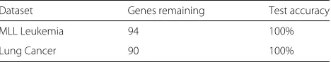
Table 7A summary of performance of gene masking with NSCC on MLL Leukemia and Lung Cancer datasets

Dataset Genes remaining Test accuracy

MLL Leukemia 94 100%

Lung Cancer 90 100%

With these sets of data, gene masking was able to pro-duce 100% training and test accuracy when the datasets were shrunk to about 400 genes using NSCC and gene masking was able to further reduce and isolate about 90 genes each. These results are highlighted in Table 7. All parameters used in these sets of experiments remained similar to those stated earlier.

It should be noted that gene masking has been derived completely off a basic binary GA. As with most evolu-tionary global optimization algorithms, the risk of getting stuck in local optima is greater when the search space is extremely large. While searching for global optimal loca-tions in a large search domain, a subsequent degradation in performance can be noted. Gene masking currently suf-fers from a similar limitation, which is highlighted by the results summarized in Table 7 for MLL and LC datasets.

Even with NSCC as the classifier that allows for an “in-built” feature selection procedure, the performance of gene masking was not as good as those with the SRBCT dataset, if dimensionality reduction is considered as a basis of performance. If the amount of shrinkage by NSCC is increased, there is a lot of loss of information solely on the basis of the magnitude of variation from the over-all mean without considering feature interdependencies. Therefore, with NSCC, MLL and LC datasets could only be shrunk to about 400 genes each prior to initializ-ing gene maskinitializ-ing. From there onwards, gene maskinitializ-ing was able to further reduce the number of genes required to maintain 100% accuracy to about 90 genes for both datasets.

Conclusion

Gene masking can be very useful in feature selection as it can isolate features that lead to high classification accu-racy. It does so by considering the impact of features on classification and heuristically removes non-contributing features. In this paper, we have demonstrated its viability by achieving 100% accuracy while significantly reduc-ing the number of genes required on SRBCT, MLL and LC datasets containing microarray gene expressions for cancers.

Funding

Publication of this article was funded by CREST, JST, Japan.

Declarations

This article has been published as part of BMC Medical Genomics Volume 9 Supplement 3, 2016. 15th International Conference On Bioinformatics (INCOB

2016): medical genomics. The full contents of the supplement are available online https://bmcmedgenomics.biomedcentral.com/articles/supplements/ volume-9-supplement-3.

Availability of data and materials

Only publicly available data has been used in this research and the cancer profiles are for SRBCT, MLL and LC available on internet [1, 23, 24].

Authors’ contributions

SL designed the gene masking concept and programmed the genetic algorithm engine. HS lead a team consisting of VVN, VWP and GS, and implemented the gene masking concept in C++ as well as carried out all experiments. HS wrote the first draft of the paper. AS, TT and SL supervised the project, and contributed in the preparation of the manuscript. All authors read and approved the final manuscript.

Competing interests

The authors declare that they have no competing interests.

Consent for publication Not applicable.

Ethics approval and consent to participate Not applicable.

Author details

1_{The University of the South Pacific, Laucala Bay, Suva, Fiji.}2_{School of} Engineering and Advanced Technology, Massey University, Palmerston North, New Zealand.3_{RIKEN Center for Integrative Medical Sciences, 230-0045} Yokohama, Japan.4_{CREST, JST, 230-0045 Yokohama, Japan.}5_{Medical Research} Institute, Tokyo Medical and Dental University, 113-8510 Tokyo, Japan.6_Griffith University, Brisbane, Australia.

Published: 5 December 2016

References

1. Khan J, Wei JS, Ringner M, Saal LH, Ladanyi M, Westermann F, Berthold F, Schwab M, Antonescu CR, Peterson C. Classification and diagnostic prediction of cancers using gene expression profiling and artificial neural networks. Nat Med. 2001;7(6):673–9.

2. Sarhan AM. Cancer classification based on microarray gene expression data using DCT and ANN. J Theor Appl Inf Technol. 2009;6(2):208–16. 3. Ghodsi A. Dimensionality reduction a short tutorial. Ontario: Department

of Statistics and Actuarial Science, Univ. of Waterloo. 2006. 4. Blagus R, Lusa L. Improved shrunken centroid classifiers for

high-dimensional class-imbalanced data. BMC Bioinforma. 2013;14(1):64. doi:10.1186/1471-2105-14-64.

5. Ghalwash MF, Cao XH, Stojkovic I, Obradovic Z. Structured feature selection using coordinate descent optimization. BMC Bioinforma. 2016;17(1):1–14. doi:10.1186/s12859-016-0954-4.

6. Marczyk M, Jaksik R, Polanski A, Polanska J. Adaptive filtering of microarray gene expression data based on gaussian mixture decomposition. BMC Bioinforma. 2013;14(1):1–12. doi:10.1186/1471-2105-14-101.

7. Holec M, Kléma J, Železný F, Tolar J. Comparative evaluation of set-level techniques in predictive classification of gene expression samples. BMC Bioinforma. 2012;13(10):1–15. doi:10.1186/1471-2105-13-S10-S15. 8. Guyon I, Weston J, Barnhill S, Vapnik V. Gene selection for cancer

classification using support vector machines. Mach Learn. 2002;46(1): 389–422. doi:10.1023/A:1012487302797.

9. Swift S, Tucker A, Vinciotti V, Martin N, Orengo C, Liu X, Kellam P. Consensus clustering and functional interpretation of gene-expression data. Genome Biol. 2004;5(11):1–16. doi:10.1186/gb-2004-5-11-r94. 10. Mamitsuka H. Selecting features in microarray classification using {ROC}

curves. Pattern Recognition. 2006;39(12):2393–404. doi:10.1016/j.patcog.2006.07.010 Bioinformatics.

York, NY, USA: ACM; 2013. p. 1034–1042. doi:10.1145/2487575.2487671. http://doi.acm.org/10.1145/2487575.2487671.

12. Sharma A, Paliwal KK. Cancer classification by gradient LDA technique using microarray gene expression data. Data Knowl Eng. 2008;66(2): 338–47.

13. Brunet JP, Tamayo P, Golub TR, Mesirov JP. Metagenes and molecular pattern discovery using matrix factorization. Proc Natl Acad Sci. 2004;101(12):4164–169. doi:10.1073/pnas.0308531101. http://www.pnas. org/content/101/12/4164.full.pdf.

14. Sharma A, Paliwal KK. A Gene Selection Algorithm using Bayesian Classification Approach. Am J Appl Sci. 2012;9(1):127–31.

15. Mitra S, Ghosh S. Feature selection and clustering of gene expression profiles using biological knowledge. IEEE Trans Syst Man Cybern Part C Appl Rev. 2012;42(6):1590–1599. doi:10.1109/TSMCC.2012.2209416. 16. Sharma A, Imoto S, Miyano S. A filter based feature selection algorithm

using null space of covariance matrix for DNA microarray gene expression data. Curr Bioinforma. 2012;7(3):289–94.

17. Sharma A, Paliwal KK, Imoto S, Miyano S. A feature selection method using improved regularized linear discriminant analysis. Mach Vis Appl. 2014;25(3):775–86.

18. Inza I, Larrañaga P, Blanco R, Cerrolaza AJ. Filter versus wrapper gene selection approaches in DNA microarray domains. Artif Intell Med. 2004;31(2):91–103. doi:10.1016/j.artmed.2004.01.007. Data Mining in Genomics and Proteomics.

19. Leung Y, Hung Y. A multiple-filter-multiple-wrapper approach to gene selection and microarray data classification. IEEE/ACM Trans Comput Biol Bioinforma. 2010;7(1):108–17. doi:10.1109/TCBB.2008.46.

20. Sharma A, Imoto S, Miyano S. A top-r feature selection algorithm for microarray gene expression data. IEEE/ACM Trans Comput Biol Bioinforma (TCBB). 2012;9(3):754–64.

21. Tibshirani R, Hastie T, Narasimhan B, Chu G. Diagnosis of multiple cancer types by shrunken centroids of gene expression. Proc Natl Acad Sci. 2002;99(10):6567–572.

22. Kumar R, Chand K, Lal SP. Gene Reduction for Cancer Classification Using Cascaded Neural Network with Gene Masking In: Sokolova M, van Beek P, editors. Advances in Artificial Intelligence: 27th Canadian Conference on Artificial Intelligence, Canadian AI 2014, Montréal, QC, Canada, May 6-9, 2014. Proceedings. Cham: Springer; 2014. p. 301–6.

23. Armstrong SA, Staunton JE, Silverman LB, Pieters R, den Boer ML, Minden MD, Sallan SE, Lander ES, Golub TR, Korsmeyer SJ. MLL translocations specify a distinct gene expression profile that distinguishes a unique leukemia. Nat Genet. 2001;30(1):41–7.

24. Gordon GJ, Jensen RV, Hsiao LL, Gullans SR, Blumenstock JE, Ramaswamy S, Richards WG, Sugarbaker DJ, Bueno R. Translation of microarray data into clinically relevant cancer diagnostic tests using gene expression ratios in lung cancer and mesothelioma. Cancer Res. 2002;62(17):4963–967.

25. Goldberg DE, Holland JH. Genetic algorithms and machine learning. Mach Learn. 1988;3(2):95–9.

26. Li T, Zhang C, Ogihara M. A comparative study of feature selection and multiclass classification methods for tissue classification based on gene expression. Bioinformatics. 2004;20(15):2429–437.

doi:10.1093/bioinformatics/bth267. http://bioinformatics.oxfordjournals. org/content/20/15/2429.full.pdf+html.

• We accept pre-submission inquiries

• Our selector tool helps you to find the most relevant journal

• We provide round the clock customer support

• Convenient online submission

• Thorough peer review

• Inclusion in PubMed and all major indexing services

• Maximum visibility for your research

Submit your manuscript at www.biomedcentral.com/submit