www.geosci-model-dev.net/10/791/2017/ doi:10.5194/gmd-10-791-2017
© Author(s) 2017. CC Attribution 3.0 License.
Total energy and potential enstrophy conserving schemes for the
shallow water equations using Hamiltonian methods –
Part 1: Derivation and properties
Christopher Eldred1and David Randall2
1LAGA, University of Paris 13, Villetaneuse, France
2Department of Atmospheric Science, Colorado State University, Fort Collins, USA
Correspondence to:Christopher Eldred ([email protected]) Received: 13 September 2016 – Discussion started: 4 October 2016
Revised: 28 December 2016 – Accepted: 4 January 2017 – Published: 17 February 2017
Abstract. The shallow water equations provide a useful analogue of the fully compressible Euler equations since they have similar characteristics: conservation laws, inertia-gravity and Rossby waves, and a (quasi-) balanced state. In order to obtain realistic simulation results, it is desirable that numerical models have discrete analogues of these proper-ties. Two prototypical examples of such schemes are the 1981 Arakawa and Lamb (AL81) C-grid total energy and po-tential enstrophy conserving scheme, and the 2007 Salmon (S07) Z-grid total energy and potential enstrophy conserv-ing scheme. Unfortunately, the AL81 scheme is restricted to logically square, orthogonal grids, and the S07 scheme is restricted to uniform square grids. The current work ex-tends the AL81 scheme to arbitrary non-orthogonal polygo-nal grids and the S07 scheme to arbitrary orthogopolygo-nal spher-ical polygonal grids in a manner that allows for both to-tal energy and potential enstrophy conservation, by combin-ing Hamiltonian methods (work done by Salmon, Gassmann, Dubos, and others) and discrete exterior calculus (Thuburn, Cotter, Dubos, Ringler, Skamarock, Klemp, and others). De-tailed results of the schemes applied to standard test cases are deferred to part 2 of this series of papers.
1 Introduction
Consider the motion of a (multi-component) fluid on a ro-tating spheroid under the influence of gravity and radiation. This is the fundamental subject of inquiry for geophysical fluid dynamics, covering fields such as weather prediction,
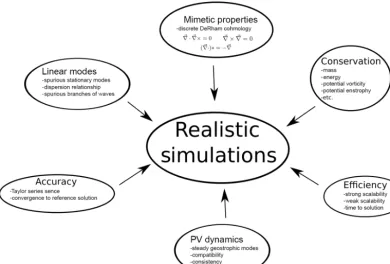
climate dynamics, and planetary atmospheres. Central to our current understanding of these subjects is the use of numeri-cal models to solve the otherwise intractable equations (such as the fully compressible Euler equations) that result. As a first step towards developing a numerical model for simulat-ing geophysical fluid dynamics, schemes are usually devel-oped for the rotating shallow water equations (RSWs). The RSWs provide a useful analogue of the fully compressible Euler equations since they have similar conservation laws, many of the same types of waves, and a similar (quasi-) bal-anced state. It is desirable that a numerical model possesses at least some these same properties (see Fig. 1, and the dis-cussion in Staniforth and Thuburn, 2012).
In fact, there exists some evidence (Dubinkina and Frank, 2007) that schemes without the appropriate conservation properties can fail to correctly capture long-term statistical behavior, at least for simplified models without any dissipa-tive effects. However, questions remain as to the reladissipa-tive im-portance of various conservation properties for a full atmo-spheric model, especially in the presence of forcing and dissi-pation (Thuburn, 2008). This subject deserves further study, but a key first step is the development of a numerical scheme that possesses the relevant conserved quantities, and is capa-ble of being run at realistic resolutions on the types of grids that are used in operational weather and climate models.
orthog-onal grids (an orthogorthog-onal grid has a dual grid with edges orthogonal to the primal grid edges) such as the latitude– longitude (lat.–long.) or conformal cubed-sphere grid. These grids are not quasi-uniform under refinement of resolution, and this leads to clustering at typical target resolutions for next generation weather and climate models (such as 2–3 km for weather; and 10–15 km for climate). Such clustering will introduce strong CFL limits, and in the case of the lat.–long. grid requires polar filtering (which is not scalable on cur-rent computational architectures) in order to take practical time steps. For these reasons, it is desirable to be able to use quasi-uniform grids such as the icosahedral grid (orthog-onal but non-square) or gnomic cubed sphere (square but non-orthogonal). In addition to the restriction to logically square, orthogonal grids, the AL81 scheme also suffers from poor wave dispersion properties when the Rossby radius is under-resolved (Randall, 1994). In fact, the unavoidable av-eraging required for the Coriolis term in a C-grid scheme is expected to lead to poor wave dispersion properties for an under-resolved Rossby radius regardless of the specific dis-cretization employed.
Recently, there has been an effort to extend the AL81 scheme to more general grids, using tools from discrete ex-terior calculus (commonly referred to as the TRiSK scheme; Thuburn et al., 2009; Ringler et al., 2010; Thuburn and Cot-ter, 2012; Weller, 2014; Thuburn et al., 2014). This has lead to the development of a family of schemes on general non-orthogonal (spherical) polygonal meshes that possess all of the desirable properties of AL81 except for extra modes branches on non-quadrilateral meshes, which are unavoid-able for C-grid schemes, and lack of either total energy or potential enstrophy conservation. It is possible to obtain one or the other, but not both at the same time. Along different lines, Salmon (2004) showed that AL81 and other doubly conservative schemes (such as Takano and Wurtele, 1982) are all members of another family of schemes on logically square, orthogonal meshes. This was done using tools from Hamiltonian methods, which are an area of active research in atmospheric model development.
Rather than using finite differences, it is also possible to extend the AL81 scheme to arbitrary grids by using compat-ible finite elements (see McRae and Cotter, 2014 and Cotter and Thuburn, 2014). Methods based on compatible finite el-ements are capable of achieving most of the properties listed in Fig. 1, and with the appropriate selection of spaces and careful mass lumping can have good linear properties as well (see Cotter and Shipton, 2012, Staniforth et al., 2013, and Melvin et al., 2014). However, these methods require the so-lution of elliptic problems at every time step, and so it is still useful to investigate a finite difference-based approach.
As an alternative to the AL81 scheme, which preserves many of its valuable mimetic properties, but has good wave dispersion properties independent of Rossby radius, Randall (1994) introduced a scheme for uniform square grids based on the vorticity–divergence formulation (termed theZgrid)
of the continuous equations. Subsequently, this approach was extended to arbitrary (spherical) orthogonal polygonal grids with a triangular dual in Heikes and Randall (1995a, b), which included the important case of an icosahedral– hexagonal grid. Although this scheme possesses many of the desirable properties from AL81, it does not conserve to-tal energy or potential enstrophy. However, a similarZgrid scheme based on a Helmholtz decomposition of the momen-tum instead of the wind, which does conserve both total energy and potential enstrophy, was developed by Salmon (2005, 2007) using techniques from Hamiltonian mechan-ics (specifically, Nambu brackets). The idea of using Hamil-tonian mechanics to derive conservative models for atmo-spheric dynamical cores has seen a great deal of interest and progress in the past 10 years (see Gassmann and Herzog, 2008; Gassmann, 2013; Sommer and Névir, 2009; Nevir and Sommer, 2009; Dubos and Tort, 2014; Dubos et al., 2015; Tort et al., 2015; Salmon, 1988; Shepherd, 2003). With the recent development of Hamiltonian formulations for essen-tially all of the equation sets and vertical coordinates used in atmospheric dynamics, it seems likely that this approach will continue to be employed in the future. Unfortunately, the scheme in S07 is defined only for planar grids, and in the key case of general polygonal grids no expression for dis-crete Hamiltonian or Casimirs was given. This precludes its further development for implementation into an operational dynamical core.
This work combines the discrete exterior calculus ap-proach from Thuburn and Cotter (2012) and the Hamilto-nian approach from Salmon (2004) to extend AL81 to gen-eral non-orthogonal (spherical) polygonal grids in a manner that conserves both total energy and potential enstrophy, and to extend S07 to arbitrary (spherical) orthogonal polygonal grids. The extension of AL81 is done through the develop-ment of a newQ(the discretization ofqkˆ×, which is also known as the nonlinear potential vorticity flux) operator, us-ing tools from Hamiltonian methods. S07 is extended by combining the Nambu bracket-based approach from Salmon (2007) with the discrete exterior calculus tools introduced in Thuburn and Cotter (2012). It should be noted that this work deals only with spatially conservative discretization. Conser-vation errors introduced due to time discretization are typ-ically much smaller than those due to space discretization. However, the extension of this approach to fully conserva-tive discretization would be a useful contribution.
con-servation properties. Section 6 discusses an implementation of these schemes, and shows some limited results. Finally, some conclusions (Sect. 7) are drawn. The appendices dis-cuss various ancillary topics such as the computational grid used (Appendix A), the specific discrete operators employed (Appendices B, C, and D), and the discrete variables used in the C- andZgrid schemes (Appendices E and F).
2 Rotating shallow water equations
The RSWs for both planar and spherical domains are pre-sented below in several forms: the vector-invariant formu-lation, the vorticity–divergence formuformu-lation, the symplectic Hamiltonian formulation based on the vector-invariant form and both Poisson bracket, and Nambu bracket formulations based on the vorticity–divergence formulations. Although all of these formulations are equivalent in the continuous case, they lead to very different discretizations.
2.1 Vector-invariant formulation
The mass continuity equation for the RSWs is expressed in vector-invariant form as
∂h
∂t +∇·(F)=0, (1)
wherehis the fluid height anduis the fluid velocity. Simi-larly, the momentum equation is expressed as
∂u
∂t +qk×(F)+∇8=0, (2) whereF=huis the mass flux,q=η
h is the potential
vor-ticity,η=ζ+f is the absolute vorticity,ζ = ˆk·∇×uis the relative vorticity,f is the Coriolis force,8=gh+K+ghs
is the Bernoulli function,hs is the topography height, andg
is gravity andK=u·u
2 is the kinetic energy.
2.2 Poisson bracket formulation (vector invariant) As discussed in Salmon (2004), let the Hamiltonian H be given by
H=
Z
1 2
h|u|2+1
2gh(h+2hs)d (3)
and letx=(h,u). Note thatdenotes the entire domain of interest, which is restricted here to either a doubly periodic plane or the sphere. Therefore, there are no boundary condi-tion to consider. The Hamiltonian formulacondi-tion can be used in the presence of boundaries, but it becomes more complicated and is not treated here. The time evolution of an arbitrary functionalFcan be written as
dF
dt = {F,H}, (4)
where the Poisson bracket{F,H}(which is a bilinear, anti-symmetric operator that satisfies the Jacobian identity) is
{F,H} = (5)
Z
d δH
δu ·∇ δF
δh − δF
δu ·∇ δH
δh +q
ˆ
k·
δH δu ×
δF
δu
.
It is useful to split this into two separate brackets as
{F,H} = {F,H}R+ {F,H}Q, (6)
where
{F,H}R=
Z
d δH
δu ·∇ δF
δh − δF
δu ·∇ δH
δh
(7)
=
Z
d δH
δh
∇·δF
δu
−δF
δh
∇·δH
δu
encompasses the gradient and divergence terms and
{F,H}Q=
Z
d
qkˆ·
δH δu ×
δF
δu
(8)
encompasses the nonlinear potential vorticity (PV) flux term. The functional derivatives δδHx of the Hamiltonian are given by
δH
δx =
8 F
. (9)
This formulation is useful for development of a scheme that possesses discrete conservation properties, as discussed be-low. A functional derivative of some functionalF[x]is de-fined as
δF
δx =lim→0
F[x+φ] −F[x]
. (10)
2.3 Conserved quantities
Since the rotating shallow water equations form a (non-canonical) Hamiltonian system, we know from Noether’s theorem and other considerations (such as the singular nature of the symplectic operator) that there are at least two cate-gories of conserved quantities: Hamiltonian and Casimirs. 2.3.1 Energy (Hamiltonian)
The first is simply the Hamiltonian itself. In this case, the Hamiltonian is the total energy of the system. Conservation of the Hamiltonian arises due to the skew-symmetric nature of the Poisson bracket. In particular, using Eq. (4) the evolu-tion ofHis given by
dH
Figure 1.A diagram of some desirable model properties for the shallow water equations, organized thematically into groups. Similar con-siderations apply for the Euler, hydrostatic primitive, and other equation sets used in atmospheric models. There is vigorous discussion in the literature and between model designers about the importance of various properties for different applications (such as weather forecasting or long-term climate prediction). The schemes presented here satisfy all of these properties, with the exception of accuracy. There are additional desirable model properties, such as consistent physics–dynamics coupling, compatible and accurate tracer advection, and tractable treatment of acoustic waves that are not presented.
since{,}is skew symmetric. For the rotating shallow water equations, the Hamiltonian is the total energy of the system. The elegant derivation of energy conservation and its sim-plicity (relying ONLY on the skew symmetry of {,}) moti-vates the use of the Hamiltonian formulation for development of numerical schemes that conserve energy.
2.3.2 Casimirs
The second category of conserved quantities consists of Casimir invariants. Since the rotating shallow water equa-tions are a non-canonical Hamiltonian system, the Poisson bracket{,}is singular and thus it possesses Casimir invari-antsCthat satisfy
{F,C} =0 (12)
for any functionalF. Note that from above, this implies that dC
dt =0. (13)
For the rotating shallow water equations, the Casimirs take the form
C=
Z
hF (q)d, (14)
whereF (q)is an arbitrary function of the potential vorticity and
δC
δx =
F (q)−qF0(q) ∇⊥F0(q)
, (15)
where∇⊥ is the skew-gradient operator. On the plane it is k×∇, and it has a coordinate-independent definition on more general manifolds such as the sphere. Important cases for F includeF=1 (mass conservation),F =q (circulation or mass-weighted potential vorticity), andF =q2
2 (potential en-strophy).
2.4 Vorticity–divergence formulation
By taking the divergence (∇·)and curl (∇⊥·) of Eq. (2), we obtain the vorticity–divergence form of the equations ∂ζ
∂t = −∇·(ηu)= −∇·(hqu), (16) ∂µ
∂t =∇
⊥·(ηu)− ∇28=∇⊥·(hqu)− ∇28, (17)
Helmholtz decomposition) as
hu=(hu)div+(hu)rot=∇χ+∇⊥ψ, (18) where(hu)div=∇χ and(hu)rot=∇⊥ψ. The stream func-tionψand velocity potentialχcan be related to the vorticity and divergence as
ζ =η−f =∇·(h−1∇ψ )+J (h−1χ ), (19) µ=∇·(h−1∇χ )+J (ψ, h−1), (20) whereJ (a, b)=∇·(a∇Tb)=∇T·(a∇b)is the Jacobian op-erator. The Helmholtz decomposition connects the vorticity– divergence formulation and the vector-invariant formula-tions. In the preceding, we have neglected the possibility of a harmonic component (a componentAfor which∇2A=0), which works because the harmonic component on the sphere is zero. On the doubly periodic plane, it would be possible to have a constant harmonic component. Finally, Eqs. (1) and (2) can be re-written in terms ofχandψdirectly as
∂h ∂t = −∇
2χ , (21)
∂ζ
∂t =J (q, ψ )−∇·(q∇χ ), (22) ∂µ
∂t =J (q, χ )+∇·(q∇ψ )− ∇
28. (23)
2.5 Poisson bracket formulation (vorticity–divergence) As shown in Salmon (2007), the preceding equations (Eqs. 21, 22, and 23) can be also be written in terms of a Poisson bracket. Let x=(h, ζ, µ) and define the Hamilto-nian
H= (24)
Z
1 2h
|∇χ|2+ |∇ψ|2+2J (χ , ψ )+1
2gh(h+2hs)d. Note that
δH=
Z
d (−ψ δζ−χ δµ+8δh) , (25)
where
8=K+gh=|∇χ|
2+ |∇ψ|2+2J (χ , ψ )
2h2 +gh+ghs, (26) which gives
δH
δx =
8
−ψ
−χ
(27)
(this is the functional derivative of the Hamiltonian with re-spect tox), and define a Poisson bracket (which is bilinear, anti-symmetric and satisfies the Jacobian identity) as
{A,B} = {A,B}µµ+ {A,B}ζ ζ+ {A,B}µζ h, (28)
where
{A,B}ζ ζ =
Z
dqJ (Aζ,Bζ), (29)
{A,B}µµ=
Z
dqJ (Aµ,Bµ), (30)
{A,B}ζ µh=
Z
dq(∇Aµ·∇Bζ−∇Aζ·∇Bµ) (31)
+(∇Aµ·∇Bh−∇Ah·∇Bµ)
for arbitrary functionalsAandB. As before, the time evolu-tion of an arbitrary funcevolu-tionalAis then given by
dA
dt = {A,H}. (32)
It is easy to see that Eqs. (21), (22), and (23) are recovered when A is set equal to h, ζ or µ, respectively. Note that each of the brackets in Eqs. (29), (30), and (31) are anti-symmetric, and that the Casimirs C=R
hF (q)d satisfy
{A,C} =0 (whereF is an arbitrary function andAis an ar-bitrary functional) independently for each bracket.
The use of the Poisson (and Nambu) bracket formulation of the shallow water equations is motivated by the intimate connection between these formulations and the conserved quantities. As is well known, the conservation of energyH
rests solely on the anti-symmetry of the Poisson bracket, and a numerical scheme that retains this feature will auto-matically conserve energy. However, potential enstrophy is a Casimir, and therefore developing a numerical scheme us-ing the Poisson formulation that conserves it requires that the discrete potential enstrophy lies in the null space of the resulting discrete bracket. This can be difficult, especially on arbitrary grids, and this motivates the use of a continuous formulation that does not contain a null space, which is dis-cussed below.
2.6 Nambu bracket formulation (vorticity–divergence) Fortunately, there is a closely related formulation of the shallow water equations in terms of Nambu brackets (see Salmon, 2007):
{F,H,Z}ζ ζ ζ=
Z
dZζJ (Fζ,Hζ), (33)
{F,H,Z}µµζ =
Z
dZζJ (Fµ,Hµ), (34)
{F,H,Z}µζ h=
Z
d
∇Zh·∇Fµ·∇Hζ·
1
∇q (35)
−∇Zh·∇Fζ·∇Hµ·
1 ∇q
+cyc(F,H,Z), where cyc is a cyclic permutation,Z=R
dh q2
product of the individual components, summed over each ba-sis (for example, in two-dimensional (2-D) doubly periodic flow the first term is ∂xZh∂xFδ∂xHζ
∂xq
. The time evolution of an arbitrary functionalAis now given by
dA
dt ={A,H,Z} = {A,H,Z}ζ ζ ζ+ {A,H,Z}µµζ (36)
+ {A,H,Z}µζ h.
These brackets are useful because they are triply anti-symmetric (which ensures the conservation ofHandZ) and non-degenerate (they have no Casimirs). In fact, discrete con-servation of both total energy and potential enstrophy re-quires only the triply anti-symmetric nature is retained. It is also possible to generalize these brackets to any Casimir (as shown in Salmon, 2005), but since we are interested mostly in potential enstrophy conservation this is not nec-essary. These brackets will form the basis of theZgrid dis-cretization method discussed below.
3 C-grid scheme
Following Thuburn and Cotter (2012), the prognostic vari-ables for the C-grid scheme are the fluid height integrated over a primal grid cell (equivalent to the mass in that grid cell) M and the wind integrated over a dual edge (equiv-alent to the circulation along a dual edge) Uˆ. Lettingx=
(M,U ), the vector-invariant Poisson bracket can be dis-ˆ cretized in a manner that preserves its anti-symmetric char-acter (which ensures total energy conservation) and a subset of the Casimir invariants (specifically mass, potential vortic-ity, and potential enstrophy). Combined with a choice for the discrete Hamiltonian, this constitutes a complete discretiza-tion for the nonlinear rotating shallow water equadiscretiza-tions. Ide-ally, one would use a Nambu bracket formulation of the vector-invariant shallow water equations rather than the Pois-son bracket formulation in order to avoid the difficulties as-sociated with developing a discretization that has the cor-rect Casimirs, since in the Nambu bracket case only anti-symmetry must be enforced. Unfortunately, the only known Nambu bracket for the vector-invariant shallow water equa-tions possesses intractable singularities and is not suitable as the basis for developing a discretization (Salmon, 2005). In what follows, uppercase letters will denote the entire (col-umn) vector of degrees of freedom, while lowercase letters will denote a specific degree of freedom. A hat on a variable indicates that the quantity is defined on the dual grid.
Specifically, the brackets in Eqs. (7) and (8) are discretized using the operators from Appendices C and B as
{A,B}R= −
δA δM
T D2δB
δUˆ
−
δA δUˆ
T D1δB
δM, (37)
{A,B}Q=
δA δUˆ
T QδB
δUˆ, (38)
where the functional derivatives are simply the partial deriva-tives with respect to the appropriate quantity. Note that these discrete brackets are only bilinear and anti-symmetric, they do not satisfy the Jacobian identity. In addition, they pos-sess only a subset of the Casimirs of the continuous brackets. Therefore, they should be properly be termed quasi-Poisson brackets. The brackets given in Eqs. (37) and (38) are essen-tially a generalization of the brackets introduced in S04 from uniform square grids to arbitrary polygonal grids, using the operators from Thuburn and Cotter (2012). The Hamiltonian
His discretized as
H=1
2gM
TI(M+2B)+1 2
ˆ
UTHC,ˆ (39) whereg is the acceleration due to gravity, B is the topo-graphic height integrated over a primal grid cell,Cˆ=MeUˆ is the mass flux on dual edges, andMe=φIM, withφ an interpolation operator. Taking functional derivatives yields δH
δx = ˆ
8 F
, (40)
where8ˆ is the Bernoulli function sampled at dual vertices andF is the mass flux integrated over primal edges. Com-puting actual values yields8ˆ =I(K+gM+gB)withK=
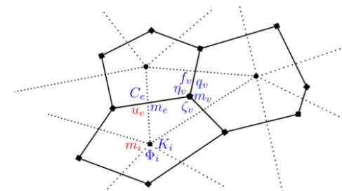
φTUˆ×2HUˆ, whereKis the kinetic energy integrated over pri-mal grid cells andF =HC. A detailed description of theseˆ discrete variables and their staggering on the computational grid can be found in Appendix E, and a diagram of their stag-gering is in Fig. 2. The resulting discrete evolution equations are
∂M
∂t +D2F =0, (41)
∂Uˆ
∂t −QF+D1
ˆ
8=0. (42)
In fact, by making alternative choices forF,Q, and 8ˆ
This is the subject of Sect. 4. A potential vorticity equation can be obtained from Eq. (42) by takingD2to yield
∂(Mˆ ×Q)
∂t −D2QF =0, (43)
where D2D1=0 has been used to eliminate the gradient term, andD2Uˆ = ˆ0 is the relative vorticity integrated over dual grid cells;ϒˆ = ˆ0+f = ˆM×Q, whereMˆ =RMis the mass integrated over dual grid cells,ϒˆ is the absolute vortic-ity integrated over dual grid cells,f is the Coriolis parameter integrated over dual grid cells, andQis the potential vorticity sampled at primal grid vertices.
3.1 Relationship to discrete exterior calculus
As discussed in Thuburn and Cotter (2012), these operators have an interpretation in terms of discrete exterior calculus. In fact,D2,D1,D2, andD1are discrete exterior derivatives, I,J, andHare Hodge stars and the various prognostic and di-agnostic quantities can be interpreted as discrete differential forms. This connection is further explored in Eldred (2015). 3.2 Linearized scheme
As is well known, the linearized version of a Hamiltonian system about a steady state can be found by evaluating the brackets at that state and using the quadratic approximation to the associated pseudo-energy as the Hamiltonian (Shep-herd, 1993). Following this procedure and letting the Corio-lis parameterf be a constant,B=0, and assuming a back-ground state ofx=(H,0), we obtain
{A,B}R= −
δA δM
T D2
δB
δUˆ
−
δA δUˆ
T D1
δB
δM, (44)
{A,B}Q=
δA δUˆ
T WδB
δUˆ (45)
for the brackets (whereW=Qqv=1is the linearized version
ofQ) and
H=1
2gM
TI(M+2B)+1 2H
ˆ
UTHUˆ (46) for the Hamiltonian, which has associated functional deriva-tives of
δH
δx = gIM
HHUˆ
. (47)
The resulting evolution equations are ∂M
∂t +H D2H
ˆ
U=0, (48)
∂Uˆ
∂t −fWH
ˆ
U+gD1IM=0. (49)
Figure 2.A subset of discrete variables and their staggering on the
computational grid for the C-grid scheme. A subscriptiindicates
quantities defined at primal grid cells or dual grid vertices, a
sub-scripteindicates quantities defined at primal or dual grid edges,
and a subscriptvindicates quantities defined at primal grid vertices
or dual grid cells. The prognostic (red) quantities are the mass
in-tegrated over primal grid cellsmi and the wind integrated along
dual grid edgesue, the other quantities are diagnostic (blue). More
details can be found in Appendix E.
3.3 Properties of scheme
This scheme has many important properties, including the following:
1. Mass and potential vorticity conservation: both massM and mass-weighted potential vorticityMˆ ×Qare con-served in both a local (flux-form) and global (integral) sense.
2. No spurious vorticity production: by construction, D2D1=0 and there is no spurious production of vor-ticity due to the gradient term in the wind equation. 3. Linear stability (pressure gradient force and Coriolis
force conserve energy): this is due to the fact thatI,J, andHare all symmetric positive definite; DT2= −D1, D2T=D1, andW= −WT.
4. Steady geostrophic modes: by construction, −RD2=
WD2(noting thatWis the same for all members of this family), which gives steady geostrophic modes. 5. PV Compatibility: again by construction −RD2=
WD2 with Qqv=c→cW, and therefore the potential
vorticity equation is compatible with the diagnostic mass equation (a constant PV field remains constant). Note that this is same as the condition required for steady geostrophic modes.
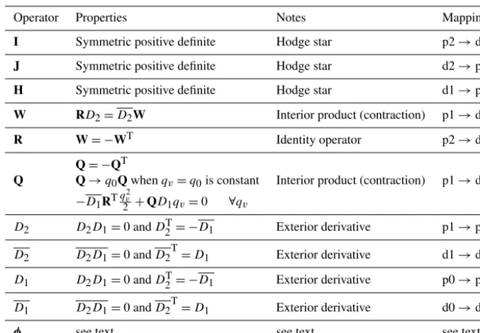
Table 1. Summary of required operator properties for obtaining the desirable mimetic properties along with total energy and potential enstrophy conservation. A example of operators that satisfy these properties can be found in Appendix C. More details can be found in Thuburn and Cotter (2012) or Eldred (2015). Note that the mapping column indicates which types of quantities the operator accepts as inputs, and what it produces as output, with “p” or “d” denoting the primal and dual grids; while the number (0,1,2) denotes the geometric
entity the quantity is integrated over. For example, theRoperator takes as input quantities integrated over primal grid cells, and produces as
output quantities integrated over dual grid cells.
Operator Properties Notes Mapping
I Symmetric positive definite Hodge star p2→d0
J Symmetric positive definite Hodge star d2→p0
H Symmetric positive definite Hodge star d1→p1
W RD2=D2W Interior product (contraction) p1→d1
R W= −WT Identity operator p2→d2
Q= −QT
Q Q→q0Qwhenqv=q0is constant Interior product (contraction) p1→d1
−D1RTq 2
v
2 +QD1qv=0 ∀qv
D2 D2D1=0 andDT2= −D1 Exterior derivative p1→p2
D2 D2D1=0 andD2
T
=D1 Exterior derivative d1→d2
D1 D2D1=0 andDT2= −D1 Exterior derivative p0→p1
D1 D2D1=0 andD2
T
=D1 Exterior derivative d0→d1
φ see text see text see text
Table 1 shows a summary of the required properties in or-der for the resulting scheme to have all of the mimetic and conservation properties discussed above.
3.3.1 Total energy conservation
Following S04, total energy will be conserved for any choice ofHif the discrete brackets retain their anti-symmetric char-acter. This requires that DT2= −D1, and that Q= −QT. The first condition is satisfied by construction of the dis-crete derivative operators D2 and D1. The second condi-tion is satisfied only for certain choices of Q. One exam-ple isQ=1
2Q eW+1
2WQ
e(as used in Ringler et al., 2010), where Qe is any function that, given the set ofqv at
pri-mal vertices, computes a uniqueQeat primal edges (such as Qe=1
2 P
v∈VE(e)qv). Flexibility in the choice ofQeallows
for a wide variety of stabilization methods such as CLUST or APVM (Weller, 2012; Weller et al., 2012). Unfortunately, this choice does not conserve potential enstrophy.
3.3.2 Potential enstrophy conservation
Following S04, potential enstrophy is a Casimir and therefore will be conserved when
{Z,A} =0 (50)
holds for any choice of functionalA. Potential enstrophy is defined as
Z=1
2(Q) Tϒˆ =1
2
ˆ
ϒ
ˆ
M !T
ˆ
ϒ. (51)
Its functional derivatives are δZ
δx =
−RQ×2Q D1Q
. (52)
Using the chain rule for functional derivatives, it suffices to show that Eq. (50) holds forA=P
imi andA=Peue.
Therefore, Eq. (50) reduces to
D2D1Q=0, (53)
−D1R Q×Q
2 +QD1Q=0, (54)
which must hold for any choice ofQ. The first of these is again satisfied by construction forD2 andD1. The second is much trickier, and is the main subject of Sect. 4. One ex-ample isQ=QeW(as used in Ringler et al., 2010), where Qe=1
2 P
v∈VE(e)qv. Unfortunately, this choice does not
3.4 Arakawa and Lamb 1981
In the case of a uniform square grid, the C-scheme grid above reduces to the well-known Arakawa and Lamb 1981 total en-ergy and potential enstrophy scheme (modified to prognose mi andue) if their choice ofQis used. Unfortunately, the
definition ofQpresented in AL81 works only for logically square, orthogonal grids. For more general, non-orthogonal polygonal grids, a new operatorQmust be found. This is the subject of the next section.
3.5 Hollingsworth instability
Since this is an extension of Arakawa and Lamb 1981 scheme, it seems extremely likely that the proposed scheme will suffer from the Hollingsworth instability, especially if applied in a height coordinate framework using a Lorenz staggering in the vertical (as discussed in Bell et al., 2016 and Hollingsworth et al., 1983). However, other similar schemes have been able to mitigate the Hollingsworth instability when used with an isentropic or Lagrangian vertical coordinate, or when a Charney–Phillips staggering is used in the vertical. On a uniform square grid using AL81, it is possible to rig-orously modify the kinetic energy stencil to eliminate the non-cancellation error that is at the heart of the instability. Furthermore, this modification can be done in such a way as to conserve total energy, by expressing it as a modifica-tion to the HamiltonianHitself and then deriving the asso-ciated consistent mass fluxFe. A similar modification of the
kinetic energy stencil for a similar C-grid scheme on non-square grids (Gassmann, 2013) has been shown to mitigate the Hollingsworth instability even without rigorous elimina-tion of the non-cancellaelimina-tion error. Therefore, given the many possible mitigation strategies, the possible presence of the instability is not expected to prevent use of this scheme in a model solving the hydrostatic or non-hydrostatic equations.
4 Operator Q
The principal novelty of the new C-grid scheme is the spec-ification of aQoperator that simultaneously conserves total energy and potential enstrophy, and also supports PV com-patibility. Previous work found choices forQthat conserved either total energy or potential enstrophy, but not both. The key lies in S04, showing that the AL81 approach could be extended to more general stencils (although retaining a logi-cally square, orthogonal grid). This work takes the Salmon 2004 approach in a different direction, keeping the same stencil as AL81 but considering a general polygonal grid. 4.1 Definition of Q
Loosely following S04,Qis defined as QFe=
X
e0∈ECP(e)
X
v∈VC(i)
qvαe,e0,vFe, (55)
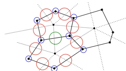
Figure 3.A diagram of the stencil ofQwhen applied to an edge
e(green). The nonlinear PV fluxQFeat edgee(green) is a linear
combination of the mass fluxesFeat the edgese0∈ECP(e)(red),
where the weightsαe,e0,v are themselves a linear combination of
the potential vorticityqvat verticesv∈VC(i)(blue), andiis the
cell shared between edgese(green) ande0(red). By choosing the
weightsαe,e0,v appropriately, an operatorQcan be found that
si-multaneously conserves both total energy and potential enstrophy and supports steady geostrophic modes.
wherei is the primal grid cell covered by botheande0. A diagram of this operator is shown in Fig. 3. An equivalent alternative form forQgiven in terms of the Poisson bracket that closely mimics the one found in S04 can be found in Eldred (2015). It is easy to see that in the case of a logically square, orthogonal grid, this approach reduces to the same stencil considered by AL81. At this point, the coefficients αe,e0,vare undetermined.
4.2 Linear system forα
It remains to determine the coefficientsαe,e0,v in a manner
such that the resulting operatorQconserves both total energy and potential enstrophy, and satisfies PV consistency. 4.2.1 Requirements introduced by energy conservation Following S04, in order forQto be energy conserving then Q= −QT. In terms of the coefficients, this implies that αe,e0,v= −αe0,e,v, or in other words, they are anti-symmetric
under an interchange ofeande0.
4.2.2 Requirements introduced by potential enstrophy conservation
From Eq. (54), in order forQto conserve potential enstrophy,
−D1RQ×2Q+QD1Q=0 must hold for any choice of Q. Expanding this out yields
X
e0∈ECP(e)
X
v∈EVC(e,e0)
αe,e0,vqv
! X
v0∈VE(e0)
te0,v0q0
Figure 4.A diagram of the stencilv∈CVE(e)=VE(i1)∪VE(i2)
with(i1, i2)=CE(e), which is simply the union of all verticesv
(blue) in the cells on either side of edgee(green).
= X
i∈CE(e)
(−ne,i)
X
v∈VC(i)
Ri,v
qv2
2 (56)
for every e, which must hold for any choice of qv. For a
given edgee, the vertices in question arev∈CVE(e)(shown in Fig. 4), where CVE(e)=VE(i1)∪VE(i2)and(i1, i2)=
CE(e). Both the left- and right-hand side of these equations are a quadratic form in this set of vertices, and for this to hold for arbitraryqvthe coefficients in these two quadratic forms
must be equal. These coefficients are linear combinations of the α’s, and therefore the equality of these quadratic forms implies a set of linear equations for theα’s.
Specifically, for each grid cell i with ne edges and nv
vertices (note that ne=nv for a polygonal grid cell, but it
is useful to keep distinct notation to ease exposition), there arenenv(n2v+1)equations (coefficients in the quadratic forms)
and nvne(n2e−1) unknowns (the coefficients αe,e0,v). Since
nv=ne, this is therefore an overdetermined system, and the
coefficient will be found through a least-squares procedure. The equations come from equating the coefficients in the two quadratic forms: there are nv(nv+1)
2 independent vertex pairs, andneedges. The unknowns are the coefficientsαe,e0,v
that are associated with the grid cell: there arene(ne−1)
2 inde-pendent unique edge pairs, and nv vertices. Note that this
has already taken into account the fact thatαe,e0,v= −αe0,e,v
(hence the wording unique edge pair), which reduces the number of independent coefficients in half. Lettingvandv0 loop over the vertices in the cell (they are the unique mem-bers of VC(i)×VC(i)), the equations are given by
Av,v=
X
e0∈EVE(v,e,i)
αe,e0,vte0,vsgn(e, e0), (57)
Bv,v=
X
i
ne,i
Ri,v
2 =
Ri,v
2 , (58)
where the sum forBv,voccurs only whenv∈VE(e); and
Av,v0 =
X
e0∈EVE(v0,e,i)
αe,e0,vte0,v0sgn(e, e0), (59)
+ X
e0∈EVE(v,e,i)
αe,e0,v0te0,vsgn(e, e0)
Bv,v0=0, (60)
whereeloops over each edge iniand EVE(v, e, i)=EC(i)∩
EV(v)−e; and sgn(e, e0)=1= −sgn(e0, e)(which ensures that the scheme is also energy conservative). A diagram of EVE(v, e, i)is provided in Fig. 5. Note that coefficients in one cell are coupled with adjacent cells whenv∈VE(e)or v0∈VE(e); that is to say, the equations involve coefficients that are associated with other grid cells. On a non-uniform mesh, this means that the entire set of coefficients must be solved at the same time.
The solution procedure outlined above gives a large matrix system
Aα=b, (61)
where each row in A represents an equation obtained by equating coefficients in the quadratic forms, and α is the vector of unknown coefficients. This system can be solved (via a least-squares approach) to yield a set of coefficients α such thatQ conserves potential enstrophy, provided the system can be solved exactly. This procedure is essentially identical to the one employed in S04. In addition, the co-efficients can be computed once, and then stored for later use. Unfortunately, the system that results directly from this procedure is impractical to solve for realistic non-uniform meshes: it is too large and ill conditioned. For example, on an icosahedral–hexagonal mesh with O(1 million) grid cells, there will be O(90 million) coupled coefficients that need to be solved for.
4.3 Practical solution
Instead, following Thuburn et al. (2009), the coefficients can be uncoupled by defining
Bv,v=
R
i,v
2 +C
ne,i, (62)
Bv,v0=Cne,i (63)
Figure 5.A diagram of the stencil EVE(v, e, i)=EC(i)∩EV(v)−
e. Consider the set(v, e, i)denoted in green; note that EVE(v, e, i)
are the two red edges. Now consider the set(v, e, i)denoted in blue:
then EVE(v, e, i)is the brown edge.
the least-squares problem is solved exactly, in the sense that the coefficients exactly satisfy the relationships for potential enstrophy and total energy conservation. Since each subsys-tem is still overdetermined, this implies the existence of an associated solvability condition. It seems likely that the solv-ability condition is the key to writing down an explicit for-mula for the coefficients in terms of Ri,v andne,i.
Unfor-tunately, we were unable to derive such a condition. How-ever, this does not prevent the numerical solution of the least-square problems, which is sufficient for practical use of the scheme. We were able to solve the systems on cubed-sphere meshes with up to 884 736 grid cells and on icosahedral– hexagonal meshes with up to 655 363 grid cells in a few hours using an unoptimized, serial algorithm on a laptop computer. Furthermore, the uncoupled nature of the prob-lem (one small independent least-squares probprob-lem per grid cell) would facilitate trivial parallelism if needed for larger meshes.
4.3.1 PV compatibility
The astute reader will note that nothing has been said yet about enforcing PV compatibility (Qqv=c=cW. It was
orig-inally believed that PV compatibility would have to added as additional equations in the matrix–vector system. However, it was found that enforcing potential enstrophy conservation (even using the uncoupled form) was sufficient to ensure that Qwas PV compatible. This corresponds with the results of S04 (Salmon, 2004), who did not explicitly add PV compat-ibility, yet all of his schemes had this property. The reasons behind this result are not yet understood. If PV compatibility had to be added explicitly, it would simply mean that
X
v∈VC(i)
αe,e0,v=we,e0 (64)
for every edge pair (e, e0); which could be easily added to the independent system of equations solved in each grid cell.
Although enforcingQqv=c=cWensures PV compatibility,
it also requires the use of theWoperator from Thuburn et al. (2009). Therefore,Qwill share the same limitations, includ-ing inconsistency on general grids. The consequences of this are explored more in Eldred and Randall (2017a).
5 Zgrid scheme
Unlike the C-grid scheme, the Z grid scheme starts with Nambu brackets rather than Poisson brackets. This greatly simplifies the derivation, since only the triply anti-symmetric nature of the brackets must be retained to ensure total energy and potential enstrophy conservation: there is no considera-tion of Casimirs. Start by defining a set of collocated discrete variables
x=(hi, ζi, µi), (65)
which are pointwise values ofh,ζ, andµat primal grid cen-ters. We will also use the More details about the grid; dis-crete operators and disdis-crete variables can be found in Ap-pendices A, D, and F.
5.1 Functional derivatives
The functional derivative of a general functionalFwith re-spect to discrete variablexiis then defined as
δF
δxi
=Fxi =
1 Ai
∂F
∂xi
, (66)
whereAi is the area of primal grid celli. The diagnostic
variables8i,χi, ψi, and qi are defined through the
func-tional derivatives of the discrete HamiltonianHand discrete Potential EnstrophyZas
8i≡
δH
δhi
=Hh, (67)
−ψi≡
δH
δζi
=Hζ, (68)
−χi≡
δH
δµi
=Hµ, (69)
qi ≡
δZ
δζi
=Zζ. (70)
At this point the discrete HamiltonianHand discrete poten-tial enstrophyZare left unspecified.
5.2 Discrete Nambu brackets
below). In addition, the bracket structure ensures that this conservation is local as well as global. That is, the evolu-tion of a conserved quantity can be written in flux form for each grid cell, where cancellation of fluxes between adjacent cells leads to the global integral being invariant. This is in contrast to a method that conserves the global integral, but cannot be written in flux form for each grid cell. In what fol-lows below, we will consider only the case whereZ is the potential enstrophy, although this approach could be easily generalized to arbitrary Casimirs (see Salmon, 2005 for an example of this on a uniform square grid). In discretizing the Nambu bracket, the operatorsD1,D2,D1, andD2from the C-grid scheme are needed. In addition to these, the additional operatorsJ (A, B),K,Xv, andXeare also needed, and they
are given in Appendix D. 5.2.1 Jacobian brackets
Loosely following S07, the{F,H,Z}ζ ζ ζbracket can be dis-cretized as
{F,H,Z}ζ ζ ζ= (71) 1
3 X edges
1
2(D1(Zζ)v)J (Fζ,Hζ)+cyc(F,H,Z).
Note that this bracket is triply anti-symmetric (due to the cyclic permutation), as required. The{F,H,Z}µµζ bracket can be similarly discretized as
{F,H,Z}µµζ =X
edges 1
2(D1(Zζ)v)J (Fµ,Hµ). (72) This bracket is only doubly anti-symmetric (in H and F
due to the anti-symmetry of J), but it will conserve Z as well provided that δµδZ
i =0 (sinceJ (A, B)=0 when either
A=0 or B=0). These brackets are essentially those en-countered when discretizing the Arakawa Jacobian, as de-tailed in Salmon (2005).
5.2.2 Mixed brackets
The mixed bracket is trickier since it contains an apparent singularity ∇1q. On closer inspection, in the continuous case this singularity cancels out when combined with the functional derivative of the potential enstrophy. This is the caveat mentioned above; i.e., the discrete mixed bracket must be constructed such that the apparent singularity cancels out with the discrete functional derivative of the potential enstro-phy. With this in mind, the general form of the discrete mixed bracket is chosen as
{F,H,Z}µζ h=X
edges D1(Zh)
D1qi
le de
(D1Fµ)(D1Hζ) (73)
−(D1Fζ)(D1Hµ)
+cyc(F,H,Z), where, from before, qi≡δδζZi. The quantities le and de are
the edge lengths on the primal and dual grid, as defined in
Appendix A. This bracket is triply anti-symmetric (again due to the cyclic permutation), and the apparent singularity will cancel ifZis chosen with care.
5.2.3 Conservation
Since the{F,H,Z}ζ ζ ζ and{F,H,Z}µζ hbrackets are triply anti-symmetric, and the{F,H,Z}ζ µµbracket is doubly anti-symmetric, both total energy and potential enstrophy will be conserved for any choice ofHandZ, provided that the caveats mentioned above are obeyed. Those are
1. δµδZ
i =0 (ensures that the {F,H,Z}ζ µµ bracket
con-serves potential enstrophy)
2. Z chosen such that the apparent singularity (D1(Zh)
D1qi
term + cyc(F,H,Z) terms) in the {F,H,Z}µζ h
bracket cancels out .
These are fairly minimal requirements, and many reasonable choices forZsatisfy them.
5.3 Discrete Hamiltonian and Helmholtz decomposition
The HamiltonianHcan be split into three parts:HFD,HJ, andHPE, where the first two are the kinetic energy due to flux-divergence terms and Jacobian terms, and the last is the potential energy. In the continuous system we have
H=HFD+HJ+HPE, (74)
where
HFD= Z
d 1
2h[∇χ·∇χ+∇ψ·∇ψ], (75)
HJ= Z
d2J (χ , ψ )
2h =
Z
dJ (χ , ψ )−J (ψ, χ )
2h , (76)
HPE= Z
d1
2gh(h+2hs). (77)
These can be discretized as
HFD= 1 2
X edges
le de
(D1χi)2
he
+ le
de
(D1ψi)2
he
, (78)
HPE= 1 2
X cells
Aighi(hi+bi), (79)
HJ= 1 2
X edges
D1
1 hv
5.4 Helmholtz decompositions and Bernoulli function By taking variations ofH, we obtain
δHPE= X cells
gAi(hi+bi)δhi, (81)
δHFD= − 1 2 X edges le de
(D1χi)2+(D1ψi)2
h2
e
δhe, (82)
−X
edges le de
(D1χi)(D1δχi)
he
+X
edges le de
(D1ψi)(D1δψi)
he
δHJ= 1 2 X edges D1 1 h2 v
δhvJ (χi, ψi)+
1 2 X edges D1 1 hv
δJ (χi, ψi).
(83) After a lot of algebra, these can be grouped (half of each term involvingδhi goes to8i and half toµi/ζi) to obtain
δH= −χiδµi+ −ψiδζi+8iδhi, (84)
where (using the definition of functional derivative) 8i =
δH
δhi
= 1
Ai
g(hi+bi)+
1 4 1 Ai Kle de (85)
(D1χi)2+(D1ψi)2
h2 e +C 2 1 Ai KD1 1 h2 v
J (χi, ψi),
µi =
1 Ai
D21 he
le deD1χi−
1 2 1 Ai D2 D1 1 hv
ψe, (86)
ζi =
1 Ai
D21 he
le
deD1ψi+ 1 2 1 Ai D2 D1 1 hv
χe. (87)
The latter two equations (Eqs. 86 and 87) are the discrete version of the Helmholtz decomposition, and form a pair of non-singular elliptic equations. They can be combined into a single equation as
A χi ψi =
FDH −JA
JA FDH χi ψi = µi ζi , (88)
where, for example,FDHχi=A1iD2h1edeleD1χi andJAψi=
1 2
1
AiD2(D1
1
hv)ψe. Note that (without the
1
Ai factors)FDHis
symmetric andJAis anti-symmetric, which means thatA= −AT(i.e.,Aitself is skew symmetric). Also note that when hi=His a constant (and thereforehe=H), they reduce to
µi=
1 H 1 Ai D2 le
deD1χi= 1
HLχi, (89)
ζi=
1 H 1 Ai D2 le
deD1ψi= 1
HLψi, (90)
where L= 1
AiD2
le
deD1, which is the expected linearization behavior.
5.5 Discrete potential enstrophy
A natural definition of the discrete potential enstrophy is
Z=1
2 X cells
Ai
η2i hi
, (91)
whereηi=ζi+fi. Taking variations of this yields
δZ
δµi
=0=Zµ, (92)
δZ
δhi
= −1
2 η2i h2i
=Zh, (93)
δZ
δζi
=ηi
hi
=Zζ. (94)
Then the natural definition forqi=ηhi
i works, and the above
simplifies to
Z=1
2 X cells
Aihiqi2, (95)
δZ
δhi
= −1
2q 2
i, (96)
δZ
δζi
=qi. (97)
By plugging these back into the{F,H,Z}µζ h bracket, it is seen that this choice ofZalso ensures that the singularity cancels.
5.6 Independence between choices forH/Zand Nambu Brackets
As noted before, the mimetic and conservation properties of the discrete scheme are completely independent of the choice of discrete HamiltonianH, provided the Hamiltonian is pos-itive definite and produces invertible elliptic equations for the Helmholtz decomposition. If the resulting elliptic equa-tions were singular, then the scheme would have a compu-tational mode (as discussed in Salmon, 2007). Additionally, the discrete Helmholtz decomposition should also simplify to a pair of uncoupled Poisson problems when linearized. The mimetic and conservation properties are also independent of the specific choice ofZ, provided that the singularity in the mixed bracket cancels andZµ=0. The given choices ofH
5.7 Discrete evolution equations
By setting F =(hi, ζi, µi)in turn, the following evolution
equations are obtained: ∂hi
∂t = −Lχi, (98)
∂ζi
∂t =Jζ(qi, ψi)−FD(qi, χi), (99) ∂µi
∂t = −L8i+Jδ(qi, χi)+FD(qi, ψi), (100) whereLis the Laplacian,FDis the flux divergence andJis the Jacobian. On an icosahedral hexagonal–pentagonal grid these operators are the same as those from Heikes and Ran-dall (1995a), and will therefore share the same limitations as those operators, such as the inconsistency of the Jacobian on general grids. The consequences of this are explored more in Eldred and Randall (2017a). The differences between the schemes arise from the use of different arguments to the oper-ators (qiinstead ofηi) and the use of different definitions for
χi andψi (which in turns induces a different Poisson
prob-lem and different expression for8i).
5.7.1 Laplacian and flux-divergence operators
The Laplacian and flux-divergence operators (which come from the mixed bracket) can be written as
Lαi=
1 Ai
D2le
deD1αi, (101)
FD(αi, βi)=
1 Ai
D2αe
le
deD1βi, (102)
whereαe=Pi∈CE(e) αi
2. 5.7.2 Jacobian operators
The Jacobian operators (which come from the Jacobian brackets) can be written as
Jδ(qi, χi)= −
1 Ai
D2[(D1qv)(χe)], (103)
Jζ(qi, ψi)=
−1 3
1 Ai
D2[(D1qv)(ψe)], (104)
+1
3 1 Ai
D2[(D1ψv)(qe)].
Note that on a polygonal grid with a purely triangular dual (including the important case of an icosahedral grid), Jδ=
Jζ.
5.8 Linearized version
Under the assumption of linear variations around a state of rest (hi =H,ζi =µi=0,qi=Hf) on afplane, this scheme
reduces to ∂hi
∂t = −Lχi = −H µi, (105)
∂ζi
∂t = − f
HLχi = −f µi, (106)
∂µi
∂t = −gLhi+ f
HLψi = −gLhi+f ζi, (107) where the Helmholtz equations given by Eqs. (89) and (90) have been used to simplify the scheme (to the point that it no longer requires solving any elliptic equations). In the case of a uniform square grid (uniform hexagonal grid), this scheme is identical to the one studied in Randall (1994) (Niˇckovi´c et al., 2002), and it shares the same excellent linear wave properties found for those schemes.
5.9 Relation to Salmon schemes
For the cases of a uniform planar square grid and a general orthogonal planar polygonal grid with triangular dual, the general discretization scheme presented above reduces to the schemes given in S07. However, this discretization scheme is more general, and it also makes specific choices for the total energyH and potential enstrophyZ when using a general polygonal grid.
5.10 Properties of scheme
The discrete scheme as outlined above possesses the follow-ing (among others) key properties:
1. Linear stability (Coriolis and pressure gradient forces conserve energy): provided thatL=LT(which is satis-fied for theLgiven above, and the majority of discrete Laplacians), the scheme will conserve energy in the lin-ear case.
2. No spurious vorticity production: by construction, the pressure gradient term does not produce spurious vor-ticity since the curl is taken in the continuous system, prior to discretization.
3. Conservation: by construction, this scheme conserves mass, potential vorticity, total energy, and potential en-strophy in both a local (flux-form) sense and global (in-tegral) sense.
4. PV compatibility and consistency: by inspection, the mass-weighted potential vorticity equation is a flux-form equation that ensures both local and global conser-vation of mass-weighted potential vorticity. In addition, an initially uniform potential vorticity field will remain uniform. This rests on the fact thatJζ(qi, ψi)=0 and
FD(qi, χi)=cLχi whenqi=cis constant.
5. Steady geostrophic modes: since the same divergence µi appears in both the linearized vorticity and
6. Linear properties (dispersion relations, computational modes): as expected, the scheme possesses the same lin-ear mode properties on uniform planar grids as those presented in Randall (1994) and Niˇckovi´c et al. (2002); and it does not have any computational modes. More details of the linear mode properties of the scheme on both uniform planar and quasi-uniform spherical grids can be found in a forthcoming paper (Eldred and Ran-dall, 2017b).
7. Accuracy: unfortunately, as shown in Heikes et al. (2013), the Jacobian operator as given is inconsistent on general grids. Even more unfortunately, the fix pro-posed in that paper breaks key properties of the Jacobian necessary to retain total energy and potential enstrophy conservation. Surprisingly, as shown in Eldred and Ran-dall (2017a), the inconsistency of the Jacobian opera-tor does not appear to cause issues in the test cases that were run. More details on possible fixes to the accuracy issue are discussed in Eldred and Randall (2017a).
6 Implementation and results 6.1 Implementation
To test the utility of the C- and Z grid schemes developed above, they were implemented in a combination of Python as a driver language along with Fortran kernels for the numer-ics. Although only tested on quasi-uniform grids that admit a structured approach, for simplicity the code uses an unstruc-tured mesh with indirect addressing. Due to this highly un-optimized implementation, no cost comparisons were made with other codes; instead, we simply note that both the C- and Zgrid schemes are structurally similar to other schemes used in existing models such as MPAS, Dynamico, and UZIM, and can be expected to share similar performance characteristics. 6.2 Results
As a short preview of the more detailed results in El-dred (2015) and ElEl-dred and Randall (2017a), a run of the Galewksy et al. (2004) test case using the C- and Z grid scheme is presented below. Third-order Adams–Bashford time stepping was used, and no dissipation beyond the in-herent damping in the time scheme was applied. The C-grid scheme was run on both a cubed-sphere grid (with 884 736 grid cells, approximately 26 km resolution, 1t=15 s) and an icosahedral grid (with 655 362 grid cells, approximately 34 km resolution, 1t=22.5 s), whereas theZ grid scheme was run only on the icosahedral grid. The absolute vortic-ity at day 6 for all three schemes is shown in Fig. 6, and the results from both the C- andZgrid schemes are broadly similar to both each other and to other results in the litera-ture. Some differences can be found in the inactive region of the jet, especially when comparing the cubed sphere to
Figure 6.A plot of the absolute vorticity from the Galewsky et al. (2011) test case at day 6 for the C-grid scheme on a cubed-sphere grid (top panel), C- grid scheme an icosahedral grid (middle panel),
andZgrid scheme on an icosahedral grid (bottom panel). The
de-veloped region of the jet is very similar for all three schemes, and is quite similar to other results in the literature. Some differences can be seen in the undeveloped region of the jet.
the icosahedral grid simulations. It is believed that these dif-ferences are due to the underlying grid structure, since the C- andZ grid scheme on the icosahedral grid produce the same pattern for the inactive region (and a very similar C-grid scheme on the cubed sphere that conserves only enstro-phy produces an extremely similar pattern to the fully con-servative C-grid scheme on the cubed sphere, as shown in Eldred, 2015). In contrast to the results in Weller (2014), we did not encounter any issues in using the C- grid scheme on the cubed-sphere grid. Plots of the time series of total energy and potential enstrophy are available in Eldred and Randall (2017a) and Eldred (2015), and verify that the schemes are conserving both energy and potential enstrophy in the spatial semi-discretization limit.
7 Conclusions
Blair Perot and Zusi, 2014). Fortunately, other than these ex-tra mode branches on the icosahedral grid the proposed C-grid scheme does not possess any additional computational modes. Furthermore, extensive testing has thus far been un-able to show negative impacts from this extra mode branch, especially when running full-physics simulations with realis-tic topography and initial conditions (John Thuburn and Bill Skamarock, personal communication, 2016).
This work has also presented an extension of the total energy and potential enstrophy conserving Z grid scheme in S07 from planar grids to arbitrary orthogonal (spherical) polygonal grids, using the same toolkit of Nambu brack-ets and Hamiltonian methods. The restriction to orthogonal grids rather than more general non-orthogonal grids (such as a cubed sphere) is a drawback. However, the major motiva-tions for using a cubed-sphere grid are the ability to prop-erly balance degrees of freedom when using a staggered C-grid methods (and therefore avoid spurious branches of the dispersion relationship), a tensor-product grid structure for spectral or finite element type methods (which ensures a di-agonal mass matrix for spectral element methods and
effi-cient implementation of finite element methods) and higher-order finite volume methods (enabling easy dimension split-ting), and an underlying piecewise continuous coordinate system for higher-order finite volume methods (allowing ex-tended stencils). None of these considerations apply to a Z grid method, so the restriction to icosahedral grids is not an-ticipated to be a significant hurdle.
A detailed comparison of the two schemes, including an analysis of the accuracy of the operators used and results from a variety of test cases, can be found in second part of this series (Eldred and Randall, 2017a). In addition, an anal-ysis of the linear mode properties of these two schemes on various quasi-uniform grids is undertaken in the third part of this paper series (Eldred and Randall, 2017b).
8 Code availability
Appendix A: Discrete grid
The schemes described above are designed to work on ar-bitrary (spherical) polygonal grids along with an associated dual grid. In the case of the C- grid scheme, the grid can be either orthogonal or non-orthogonal, while theZgrid scheme is restricted to orthogonal grids. A description of the grid framework is given in what follows.
A1 General non-orthogonal polygonal grid
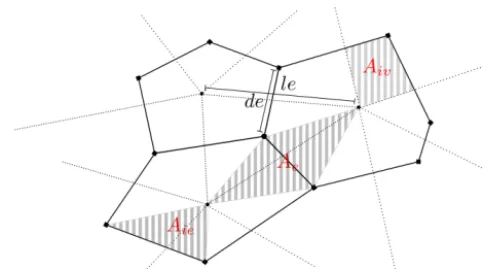
Consider a (primal) conformal grid constructed of polygons (or spherical polygons). A dual grid is constructed such that there is a unique one to one relationship between elements of the primal grid and element of the dual grid: primal grid cells are associated with dual grid vertices, primal grid edges are associated with dual grid edges, and primal grid vertices are associated with dual grid cells. This grid configuration covers the majority of grids that are used in current and upcoming atmospheric dynamical cores, including cubed sphere and icosahedral grids (both hexagonal–pentagonal and triangular variants). Once the dual grid vertices have been placed, there are several important geometric quantities that are needed in order to construct the discrete operators (shown graphically in Fig. A1). Specifically, we need the primal cell areaAi, the
dual cell area Av, the distance between primal grid centers
“le”, the distance between dual grid centers “de”, and the overlap areas Aiv andAie. On a planar grid, these are
eas-ily defined using the standard Euclidean metric and formu-las. On a spherical grid, distances must be calculated using geodesic arcs, and areas are calculated by subdividing into spherical triangles as needed and then applying the relevant spherical area formulas. See the discussion in Weller (2014) for more details.
Appendix B: Discrete derivative operators
Following Thuburn and Cotter (2012), a set of discrete derivative operators can be defined as
D1= X
v∈VE(e)
te,v, (B1)
D1= X
i∈CE(e)
−ne,i, (B2)
D2= X
e∈EC(i)
ne,i, (B3)
D2= X
e∈EV(v)
te,v, (B4)
wherene,iis an indicator that is 1 wheneis oriented out of a
primal grid cell and−1 wheneis oriented into a primal grid cell, andte,vis an indicator that is 1 wheneis oriented into
a dual grid cell and−1 wheneis oriented out of a dual grid cell.D2is the divergence,D2is the curl,D1is the skew gra-dient, andD1is the gradient; by the Gauss theorem these are
Figure A1.The geometric quantities on a planar grid. Primal grid edge lengths are denoted as “de”, dual grid edge lengths are denoted
as “le”, the area associated with an edge byAe, the overlap between
primal grid celliand edgeebyAie, and the overlap between dual
grid cellvand edgeebyAiv. Note that the same definitions can
be used on a spherical grid, provided the appropriate measures are used (such as geodesic lengths for distances, and spherical polygo-nal areas for areas). See Weller (2014) for more details.
exact (since they operate on integrated quantities). By con-struction, these satisfy D2D1=0, D2D1=0, D2T= −D1 andD2
T
=D1for arbitrary polygonal grids. These identities are the discrete analogues of∇·∇⊥=0,∇⊥·∇=0, and ad-jointness between divergence and gradient, and curl and skew gradient. The operators can also be identified as the discrete exterior derivative operators from discrete exterior calculus.
Appendix C: Specific choices for various C-grid operators
In order to close the C-grid scheme presented in Sect. 3, spe-cific choices must be made forI,J,H,R,φ, andW. The ones used here (and in Ringler et al., 2010 and Thuburn et al., 2014) are
I= 1
Ai
, (C1)
HO= X
i∈CE(e)
le
de, (C2)
HNO= X
e06=e∈S(e)
He,e0, (C3)
J= 1
Av
, (C4)
φ= X
i∈CE(e)
Aie
Ae
, (C5)
R= X
i∈CV(v)
Aiv
Ai
and
W= X
e0∈ECP(e)
We,e0, (C7)
whereI,J, andH0are diagonal matrices,HOis used on or-thogonal grids such as the icosahedral grid andHNOis used on non-orthogonal grids such as the cubed-sphere grid. The details of the construction of this operator, including the sten-cilS(e)and the weightsHe,e0, can be found in Thuburn et al.,
2014). The weights We,e0 are chosen such that W= −WT
and−RD2=D2W(the details for this operator can be found in Thuburn et al., 2009).I,H, andJtransform quantities be-tween the primal and the dual grids, and are in fact what are known as discrete Hodge star operators.Ris a discrete analogue of the identity operator that maps quantities inte-grated over primal cells to quantities inteinte-grated over dual cells, while W can in fact be identified as a discrete ana-logue of the interior product (or contraction) operator. On an orthogonal grid, the choices given forI,J, andHcorrespond to the Voronoi Hodge star from discrete exterior calculus.
Appendix D: Specific choices for variousZ-grid operators
For theZgrid scheme, the following operators are needed: K= X
e∈EC(i)
, (D1)
which is the sum of edges for a given grid cell, and
J (A, B)=ne,2A2B1+ne,1A1B2, (D2) which is used to build a discrete Jacobian operator. Note that J (A, B) is anti-symmetric (J (A, B)= −J (B, A)) and satisfiesJ (A,0)=J (B,0)=J (A, A)=0. In addition, two different interpolations (from cell centers to vertices and to edges, respectively) are defined:
Xv=
X
i∈CV(v)
CXi, (D3)
Xe=
X
i∈CE(e)
1
2Xi, (D4)
where C- is a constant given by 1n, andnis the size of CV(v) (equal to 4 for quadrilateral dual grid cells and 3 for triangu-lar dual grid cells).
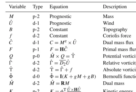
Table E1.List of discrete C- grid variables and their diagnostic equations.
Variable Type Equation Description
M p-2 Prognostic Mass
ˆ
U d-1 Prognostic Wind
B p-2 Constant Topography
f d-2 Constant Coriolis force
ˆ
C d-1 C=Me× ˆU Dual mass flux
F p-1 F=HCˆ Primal mass flux
Q p-0 Mˆ ×Q= ˆϒ Potential vorticity
ˆ
0 d-2 0ˆ=D
2Uˆ Relative vorticity
ˆ
ϒ d-2 ϒˆ = ˆ0+f Absolute vorticity
ˆ
8 d-0 8ˆ =I(K+gM+gB) Bernoulli function
ˆ
M d-2 Mˆ =RM Dual mass
K p-2 K=φTUˆ×2HUˆ Kinetic energy
Table F1.List of discreteZgrid variables and their diagnostic equa-tions.
Variable Type Description
hi Prognostic Fluid height
ζi Prognostic Relative vorticity
µi Prognostic Divergence
ηi=ζi+fi Diagnostic Absolute vorticity
qi=ηi/hi Diagnostic Potential vorticity
8i=Ki+ghi Diagnostic Bernoulli function
Ki Diagnostic Kinetic energy
χi Diagnostic Velocity potential
ψi Diagnostic Stream function
Appendix E: Discrete variables for the C-grid scheme Table E1 gives the discrete variables used in the C- grid scheme, their type (which indicates the staggering on the grid), and their diagnostic equation (where applicable). For the type, the first designator indicates the location on the grid type (primal or dual) and the second designator indicates the degree of the geometric entity the quantity is integrated over (0,1 or 2). For example, C- is a quantity on the dual grid in-tegrated over edges.