Original Article
Estimation of excess hazard using compound Poisson frailty model
Mahmood Sheikh Fathollahi1, Mahmood Mahmoodi2*, Kazem Mohammad2, Hojjat Zeraati2, Arash Jalali2
1 Department of Social Medicine and Occupational Environment Research Center, Medical School, Rafsanjan University of Medical Sciences, Rafsanjan, Iran
2 Department of Epidemiology and Biostatistics, School of Public Health, Tehran University of Medical Sciences, Tehran, Iran
ARTICLE INFO ABSTRACT
Received 07.04.2014 Revised 21.07.2014 Accepted 07.09.2014 Published 20.2.2015
Available online at: http://jbe.tums.ac.ir
Background & Aim: The excess hazard rate proposed by Andersen and Vaeth may underestimate
the long-term excess hazard rate for cancer survival. Zahl explained the phenomenon by continuous selection of the most robust individuals after diagnosis. He applied correlated inverse Gaussian and gamma frailty models to estimate excess intensity and reached a better estimate of the rate and called it the corrected excess hazard. The compound Poisson distribution has more parameters and therefore owns more flexibility and includes gamma and inverse Gaussian distributions as special cases. Therefore, the aim of this study was to estimate the excess hazard using compound poisson frailty model
Methods & Materials: Both shared and correlated frailty (CF) variables based on compound
Poisson distribution were used to model unobserved common covariates. A data set of patients diagnosed with localized or regional gastrointestinal tract cancer collected at the Mazandaran province of Iran was studied. As registration systems in Iran are so affected by omission and various errors, a number of five West Coale- Demeny life tables for men and four for women were constructed corresponding to each birth cohort, which was considered as the reference life tables. Thus, population-based mortality rates [h1(t)] were simply replaced by the appropriate values of the West tables depending on the sex (male or female) and birth cohort of the patient.
Results: The CF model with unequal variances could best estimate the long-term excess hazard. Conclusion: This study advocates the CF models can best estimate the long-term excess hazard
rates regardless of the distribution of the frailty variable. Key words:
excess hazard, frailty models, shared and correlated frailty models,
gamma and inverse Gaussian frailty models, compound Poisson frailty model,
Coale–Demeny life table models,
Mazandaran province of Iran
Introduction1
Excess mortality modeling is a statistical tool frequently used in population-based studies to evaluate the effect of a particular disease on mortality, especially when the cause of death is known unreliable or unavailable (1, 2). Zahl noted that the excess hazard rate proposed by
* Corresponding Author: Mahmood Mahmoodi, Postal Address:
Department of Epidemiology and Biostatistics, School of Public Health, Tehran University of Medical Sciences, P.O. Box: 14155-6446, Tehran, Iran. Email: [email protected]
Gaussian and gamma frailty models to estimate excess hazard in malignant melanoma or colon cancer patients (4, 5).
The compound Poisson distribution was introduced by Aalen as a frailty distribution (6, 7). The distribution is considered as a hit model, where each individual experiences a random number of hits causing damage, each of a random size. It includes power variance function (PVF) distribution, gamma, and inverse Gaussian distribution as special cases. The model was successfully used by Aalen in 1992 (7) to model the incidence of marriage of women born in Denmark. Hougaard et al. in 1994 (8) applied the model to diabetic nephropathy onset data. Aalen and Tretli in 1999 (9) applied the compound Poisson distribution to testicular cancer data. Haukka et al. in 2003 (10) applied the model to schizophrenia data from the Finnish population born 1950 to 1968.
In estimating excess hazard, life tables as the common tools comprising mortality information of the general population are considered as a standard reference and one usually relies on the published life tables as the reference mortality rate that depends on the characteristics of the study patient, such as sex, and age, and year of birth. One major limitation of these reference life tables is that individuals in a population basically come from different cohorts with different mortality experiences, whereas information of mortality rates of different cohorts is as if pooled and combined into a single table. This disparity in the pattern of mortality across cohorts can severely affect life table figures and therefore excess mortality measures, which requires an adequate adjustment for birth cohort effect during the establishment process of life tables. Unfortunately, in many developing countries including Iran, registration systems either do not exist or are so affected by omission and other errors. Indeed, there may be little known on the actual age pattern of mortality in these populations, so as measures based on the data that they produce fail to reflect properly either levels or trends of mortality. A number of model life table systems have been developed for use in such cases, but one of the most commonly used
is the Coale- Demeny model life tables for developing countries (11-13).
Since a dramatic climb was evident in incidence rate of gastrointestinal (GI) tract cancers in northern regions of Iran during the past a few decades (14, 15), we came to examine the long-term excess mortality due to the GI tract cancer in Mazandaran, the province with the dominating rate of GI tract cancers (15) using the shared and correlated compound Poisson frailty models. To do so, we constructed distinct life tables for different cohorts, each separated by gender, using the West Coale- Demeny life table model and these tables were considered as the population-based mortality rates.
Compound Poisson Frailty Model
The compound Poisson distribution was introduced by Aalen (1988, 1992) as a frailty distribution (6, 7). The distribution can be established as the sum of a Poisson-distributed number of independent and identical gamma distributed random variables.
Z = X + X + X + ⋯ + X ; if N > 0,0 ; if N = 0,
where N is Poisson distributed with the expectation υ[N ~ Poisson(υ)], while X1, X2, X3, … are independent and gamma distributed with Xi ~ Γ(k, λ).
Using the following parameterization:
υ = −kλγ , λ = λ, k = −γ,
the Laplace transform of the compound Poisson distribution takes the form
L s = exp "−kγ # λ + s − λ $%
Expectation and variance of a compound Poisson-distributed random variable Z are
E Z = kλ ' , Var Z = k 1 − γ λ '
Applying the Laplace transform given above, the marginal survival and hazard functionin case of a compound Poisson frailty model are as
S t = exp "−kγ # λ + Λ t − λ $%
and
λ/ t = kλ t λ + Λ t '
Using the constraint EZ = 1, it holds
and accordingly
Var Z =1 − γλ
In consequence, after some simplification (16)
0 t = exp 1− '23451 + 2 3
' Λ t 6 − 178 (1)
and the observed population mortality rate is further given by
λ/ t = 9 :
5 ;=>?<3@ : 6=>? (2)
In case γ = 0 or γ = 0.5 the gamma or inverse
Gaussian distributions will be yielded as special cases.
A Shared Frailty (SF) Model
Consider an individual with common frailty Z for
both dying of cancer and of other causes. The individual intensity is then described by (4, 5) λ t; Z = zBh t + h t D, (3)
where t denotes time from diagnosis to death for individual i, and Z is a compound Poisson variable. Here, h1(t) is known as the intensity for
dying of other causes, or the basic mortality rate for an individual, and is usually assumed of the Gompertz-Makeham form, that is, h1(t) = a + b
exp[c(t0 + t)], where a, b, and c are the
parameters of the Gompertz-Makeham distribution, and t0 is age at diagnosis; t0 + t is
the current age. h2(t) is the individual cancer
intensity, and can be of Weibull form, and is interpreted as the force of dying of the cancer under study. This model is called a “ shared compound Poisson frailty model because the frailty variable is common to both intensities.
The survival function for the population is according to Hougaard (17) and Eq. (1)
s T = EXP 1−1 − γγσ 451 +1 − γ H tσ
+ H t 6 − 178
in which H1(t) is the cumulative basic
mortality rate and H2(t) is the cumulative
individual cancer mortality.
The observed population mortality is then
given by using Eq. (2) as
λ/ t = h t + h t
I1 + σ1 − γ H t + H t J ' which may be written as
λ/ t = hK t + hK t
LMhK t − N=:
I ;=>?<3 O=: ;O3: J
=>?P M+hK t −
N3 :
I ;=>?<3 O=: ;O3 : J
=>?PQ (4)
where
hKR t = hKR t 51 + σ1 − γ HR t 6
' ; i = 1,2
(5)
As Zahl stated, hKR t is denoted the population cancer hazard as this function describes the force of dying of the cancer under study for the study group, and this is what we intend to estimate by the excess hazard model. The last term in Eq. (4) is the bias of the excess intensity model, and this is also a measure of the increase in the risk of dying of other causes after removing the risk of dying of cancer. The shared frailty model will be denoted by SF below.
A Correlated Compound Poisson Frailty Model
The shared frailty model has important shortcomings. First, an individual may have distinct frailties for h1(t) and h2(t). Second, the
variances of the two frailty variables may differ and the difference may be large (6). A suggested way of handling this problem is by establishing a multivariate distribution by adding up a number of independent frailty variables. Here, the individual mortality rate is described by (4, 5). λ t; Z , Z = Z h t + Z h t
where Zi, i = 1,2, are two mixed compound
Poisson variables with variances σ and σ , respectively. The correlation coefficient between the two variables is further denoted by 0 ≤ ρ ≤ min X2=
23,
23
2=Y. The population intensity
λ/ t = hK t + hK t
−Z '2=23[σ \hK t − N=:
5 ;=>?= X2=3O=: ;233O3: Y6 =>?] +
σ \hK t − N3:
5 ;=>?= X2=3O=: ;233O3: Y6=>?]^ (6)
where
hKR t = N_ : ` ;=>?<_3 O_ : a
=>?; i = 1,2; (7)
Once more, the last term in Eq. (6) is the bias when the two frailty variables are correlated.
hK t can be estimated indirectly and the estimate is as Zahl stated the corrected excess hazard
We have that Eq. (6) equals Eq. (4), when
ρ = 1 and Z1 and Z2 have equal variances
(σ1 = σ2).
When σ1 = σ2, this model will be denoted by
CF1, otherwise this model is denoted by CF2.
Cancer Survival
Estimation
The population cancer hazard, hK t , is estimated indirectly by substituting a known function for h1(t) in the likelihood for the shared
and correlated frailty (CF) models, a method which “ does not require exact information about the cause of death. Furthermore, this indirect method reduces the number of parameters to be estimated. In this method, we simply substitute the population mortality rate for h1(t), assuming
this equal to the individual risk of dying from diseases other than the cancer under study. The individual cancer mortality h2(t) is assumed of
Weibull form. The parameters of the frailty distribution and h2(t) are estimated by the
maximum likelihood method.
Creating the West life table model
Since in many countries including Iran, death registration is incomplete or nonexistent, adequate life tables cannot be calculated from the data available. Model life tables have been developed for use in such cases. The Coale
-Demeny model life tables are amongst the most commonly used models and consist of four sets or models, each representing a distinct mortality patterns, including North, South, East, and West. As the West pattern is considered to represent the most general mortality pattern, Coale and Demeny recommended its use when reliable information is not available for choosing one of the other patterns (13). Plus, our previous experience reveals that the West life table model can best estimate the actual age pattern of mortality of our population (18). Having the measure of infant mortality rate (IMR) for each year of birth, defined as the number of newborns dying under a year of age divided by the number of live births that year, Coale- Demeny model life tables can be constructed showing mortality rate for single years of age 0- 100. Concerning the Mazandaran province, IMR was available for birth years after 1965; therefore, linear extrapolation methods were invoked to approximate IMR for birth years before 1965. Because the study patients came from different birth cohorts with experiencing different mortality patterns, men were classified into five distinct cohorts of 1911-1920, 1921- 1930, 1931- 1940, 1941- 1950, and 1951- 1961, and women into four cohorts of 1921- 1930, 1931 -1940, 1941- 1950, and 1951- 1961. It should be noted that to establish life tables, an average IMR was obtained for each cohort and according to gender. As such a number of five West life tables for men and four tables for women were constructed for Mazandaran province of Iran, corresponding to each birth cohort. Once the West life tables were established, population-based mortality rates [h1(t)] were simply
replaced by the appropriate values of the West tables depending on the sex (male or female) and birth cohort of the patient.
Gastrointestinal tract cancer
a maximum period of 15 years by the year 2006. The study was approved by the Ethics Committee of Tehran University of Medical Sciences.
Results
The mean age of the patients was 58.26 ± 10.90 (mean ± SD) years (range 40- 90). Males accounted for 66.3% and females 33.7% of GI tract cancers. The Kaplan- Meier method of survival analysis estimated that the survival rates in 5, 10, and 15 years following diagnosis were 16.9%, 13.8%, and 6.2%, respectively. The overall patient survival rate was not statistically different across the three subgroups of patients with esophageal, stomach, and colorectal cancers (log-rank test; P = 0.213). Owing to small sample size, especially the few number of patients with colorectal cancer, we analyzed the whole sample as patients with GI tract cancer,
and did not carry out distinct analysis for each type of GI cancer.
Table 1 presents parameters for the shared and CF models. The individual cancer hazard h2(t) was assumed of the two-parameter Weibull
form. As shown in table, in all models β was estimated to be more than 1 indicating an increasing individual cancer hazard h2(t) over
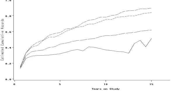
the course of study. The log-likelihoods are almost identical for all models, but the correlation coefficients for CF1 and CF2 models are different. The correlation coefficients are positive meaning that the risk of dying of cancer is correlated to the risk of dying of other causes. The frailty parameters are estimated with inflated standard errors in all models, which may be reduced by studying larger datasets. In figure 1, we present the integrated excess intensity (traditional excess hazard) comparing with the integrated corrected excess hazards.
Table 1. Estimated parameters for 484 patients with GI tract cancer diagnosed in Mazandaran province of Iran, and according to
the West Coale–Demeny regional life table model (based on compound Poisson frailty distribution)
Model Parameters of Weibull distribution Parameters of frailty distribution −ln(L)
β η Σ σ١ σ٢ ρ
SF 1.25 (0.39) 0.26 (0.09) 1.95 (0.51) - - - 521.07
CF1 1.19 (0.27) 0.20 (0.06) 1.92 (0.43) - - 0.55 (0.47) 520.61 CF2 1.13 (0.25) 0.19 (0.07) - 1.80 (0.59) 2.21 (0.94) 0.75 (0.66) 519.84
GI: Gastrointestinal, SF: Shared frailty model, CF1: Correlated frailty model with equal variances, CF2: Correlated frailty model with unequal variances. Standard errors are given in parentheses
Figure 1. Integrated corrected excess hazards compared with integrated
Table 2. Estimated cumulative excess mortality for 484 patients with GI tract cancer diagnosed
in Mazandaran province of Iran according to shared and correlated frailty models and based on the compound Poisson frailty distribution
Model Years on the study
2 5 10 15
Conventional excess hazard 0.30 0.32 0.37 0.51 Compound Poisson frailty model
Shared 0.46 0.59 0.78 0.90
Correlated with equal variances 0.42 0.56 0.75 0.84 Correlated with unequal variances 0.36 0.44 0.55 0.62
GI: Gastrointestinal
As can be seen, after 2 years the difference increases. The corrected excess hazard based on the CF2 model gives the best estimate of the long-term cause-specific mortality, while the SF and CF1 models give the worst fit. Modeling of the heterogeneity, especially by distinct variances for Z1 and Z2, is an essential way for
capturing the selection phenomenon.
Table 2 depicts the estimated cumulative excess mortality both traditional and corrected counterparts for 484 patients with GI tract cancer diagnosed in Mazandaran province of Iran. It is evident that the corrected estimates differ from the traditional estimates and the difference increases, especially after 2 years indicating the phenomenon of systematic selection of robust individuals after diagnosis (that means patients with low frailty) may probably be taken place.
Discussion
Here, we tried both shared and correlated frailty models based on compound Poisson distribution for estimating long-term excess hazard rate. An interesting interpretation of this distribution is that individuals may come from different backgrounds and cultures and are exposed to different environmental effects which cause each individual experiences several hits causing damage, so as the number of hits causing damage in an individual are random and each of a random size. The effect of these hits accumulates over time and increases individual frailty (6, 7). Furthermore, because there are more parameters in the distribution compared to gamma and inverse Gaussian, it will increase the flexibility of the model. That is why we found it relevant to model excess hazard rate.
Even though, the individual cancer hazard was parameterized for getting small standard errors and there were more parameters in the model when compared to former competing risks models (4, 5), hence naturally leading to more flexibility of the model, the correlation coefficients and the variances were not estimated with small standard errors which might be reduced by studying larger datasets.
Heterogeneity as the responsible for systematic selection process of robust individuals after diagnosis may be happened in our study. A considerable number of deaths (366 deaths, i.e., 75.6% of the total sample size) occurred in the first early years of diagnosis showing those patients who were most frail or those who were diagnosed in higher stages of the disease would die earlier than the others and, in consequence, systematic selection of robust individuals after diagnosis (that means patients with low frailty) would have been probably taken place.
It should also be alludedthat we observed a huge number of deaths in the first 2 years of diagnosis so a dramatic climb was observed in excess mortality during the period in all models, as figure 1 shows. This might be expected because patients with GI tract cancers are generally discovered at a late stage of disease when cancer is difficult to cure successfully at this stage (19, 20).
mortality in our population. The basis of the Coale- Demeny life table system is the mortality patterns exhibited in 192 actual life tables by sex. Analysis of 192 life tables revealed four age patterns of mortality labeled North, South, East, and West. The West pattern is, however, derived from the largest set of observed life tables (130) and is considered to represent the most general mortality pattern. They recommended its use when the reliability of information is under question for choosing a more deserved model (12, 13, 21).
Here, we address how to correct the excess hazard rates when there is unobserved correlated heterogeneity. This study advocates the correlated frailty models with unequal variances can best estimate the long-term excess hazard regardless of the distribution of the frailty variable.
Acknowledgments
This study was made possible by the financial support of Tehran University of Medical Sciences. We would like to extend our special gratitude to Babol Cancer Registry for kindly providing us with the data set used in this paper.
References
1. Buckley JD. Additive and multiplicative models for relative survival rates. Biometrics 1984; 40(1): 51-62.
2. Nelson CP, Lambert PC, Squire IB, Jones DR. Flexible parametric models for relative survival, with application in coronary heart disease. Stat Med 2007; 26(30): 5486-98. 3. Andersen PK, Vaeth M. Simple parametric
and nonparametric models for excess and relative mortality. Biometrics 1989; 45(2): 523-35.
4. Zahl PH. Correlated frailty models; modelling of unobserved correlated risks of deaths. Norwegian J Epidemiol 1994; 4: 64-8.
5. Zahl PH. Frailty modelling for the excess hazard. Stat Med 1997; 16(14): 1573-85. 6. Aalen OO. Heterogeneity in survival
analysis. Stat Med 1988; 7(11): 1121-37. 7. Aalen OO. Modelling heterogeneity in
survival analysis by the compound poisson distribution. Ann Appl Probab 1992; 2(4):
767-1033.
8. Hougaard P, Myglegaard P, Borch-Johnsen K. Heterogeneity models of disease susceptibility, with application to diabetic nephropathy. Biometrics 1994; 50(4): 1178-88.
9. Aalen OO, Tretli S. Analyzing incidence of testis cancer by means of a frailty model. Cancer Causes Control 1999; 10(4): 285-92. 10. Haukka J, Suvisaari J, Lonnqvist J.
Increasing age does not decrease risk of schizophrenia up to age 40. Schizophr Res 2003; 61(1): 105-10.
11. United Nations. Model life tables for developing countries. New York, NY: United Nations; 1982.
12. United Nations. Manual X: Indirect techniques for demographic estimation. New York, NY: United Nations; 1982.
13. Coale AJ, Demeny P. Regional model life tables and stable populations. 2nd ed. New
York, NY: Academic Press; 1983.
14. Sadjadi A, Nouraie M, Mohagheghi MA, Mousavi-Jarrahi A, Malekezadeh R, Parkin DM. Cancer occurrence in Iran in 2002, an international perspective. Asian Pac J Cancer Prev 2005; 6(3): 359-63.
15. Cancer Control Office of Ministry of Health. Iranian annual cancer registration report 2003. Tehran, Iran: Kelk-e-Dirin Publication; 2005 [In Persian].
16. Wienke A, Ripatti S, Palmgren J, Yashin A. A bivariate survival model with compound Poisson frailty. Stat Med 2010; 29(2): 275-83. 17. Hougaard P. Life table methods for
heterogeneous populations: distributions describing the heterogeneity. Biometrika 1984; 71(1): 75-83.
18. Mohebbi M, Mahmoodi M, Wolfe R, Nourijelyani K, Mohammad K, Zeraati H, et al. Geographical spread of gastrointestinal tract cancer incidence in the Caspian Sea region of Iran: spatial analysis of cancer registry data. BMC Cancer 2008; 8: 137. 19. Paz IB, Hwang JJ, Iyer, VI. Esophageal
cancer. In: Pazdur R, Coia LR, Hoskins WJ, Wagman LD. Cancer management: a multidisciplinary approach. 11th ed. New
20. Blanke CD, Coia LR, Schwarz RE. Gastric cancer. In: Pazdur R, Coia LR, Hoskins WJ, Wagman LD. Cancer management: a multidisciplinary approach. 11th ed. New
York, NY: CMP United Business Media;
2008. p. 273-86.
21. Siegel JS, Shryock HS, Stockwell E, Swanson DA. The Methods and materials of demography. 2nd ed. New York, NY:
Appendix
Let k1, k2, and k3 be some real positive variables
and let Y1, Y2, and Y3 be independently
compound Poisson distributed random variables with Y1 ~ cP(γ, k1, λ), Y2 ~ cP(γ, k2, λ), and Y3 ~
cP(γ, k3, λ). Thus,
E YR = kRλ ' , Var YR = kR 1 − γ λ ' ; i=1,2
The frailty variables Z1 and Z2 can be defined
as a set of the three above independent compound Poisson variables using a similar additive structure for the frailties as in gamma and inverse Gaussian models
Z = Y + Y ⇒ E Z
= k + k λ ' , Var Z
= k + k 1 − γ λ '
Z = α Y + Y ⇒ E Z
= α k + k λ ' , Var Z
= α k + k 1 − γ λ ' where α is a scaling parameter (a positive real
number).
Furthermore, the following relations are assumed:
E Z = k + k λ ' = 1, E Z =
α k + k λ ' = 1 , which leads to
Var Z =1 − γλ , Var Z = α 1 − γλ
The two above equations result in α =233 2=3 The covariance between Z1 and Z2 is given by
Cov Z , Z = E Z Z − E Z E Z
In order to derive an expression for the first term on the right-hand side of the above equation we require
E Y = Var Y + BE Y D = k 1 − γ λ ' + k
We then have for the first term on the right-hand side of the covariance equation
E Z Z = EB Y + Y × αD Y + Y
= αEBY + Y Y + Y Y + Y Y D = αBk 1 − γ λγ−2+ k λ2γ−2+
k k λ2γ−2+ k k λ2γ−2+ k k λ2γ−2D
= αBk 1 − γ λγ−2+ k +k k +
k λ2γ−2D
= αBk 1 − γ λγ−2+ α' D
= αBk 1 − γ λγ−2+ 1D
E Z E Z = 1
Furthermore, Z1 and Z2 are correlated since
they contain the common part Y1 with a
correlation coefficient:
ρ = ijk =, 3 lmno KKKKKKKKKKKKKKKKKKKKKKK=mno 3 =
pq= ' 9?>3
rB qKKKKKKKKKKKKKKKKKKKKKKKKKKKKKKKKKKKKKKKKKKKKKKKKKKKKKKKKKKKK=;q3 ' 9?>3DBp3q=;qs ' 9?>3D
=
q= r qKKKKKKKKKKKKKKKKKKKKKKKKK=;q3; q=;qs
Because the k-parameters are all assumed non-negative, it follows that the range of the correlation between frailties depends on the values of σ1 and σ2:
0 ≤ ρ ≤ min Iσσ ,σσ J
We can derive the unconditional model, applying the Laplace transform of compound Poisson distributed random variables. The population survival probability becomes
S t = t t t expB− y + y H t −wv wv wv α y + y H t D. f y . f y . f y dy dy dy
= exp z−q=# λ + H t + αH t − λ ${ ×
exp z−q3|}λ + H t ~ − λ •{ ×
exp z−qs|}λ + αH t ~ − λ •{ The following relations are hold:
λ = 1 − γσ , α =σσ
k = ρ2= 23X
' 2=3Y
' ,
k = X2'
= 3Y
'
X1 − ρ2= 23Y,
k =2=2
3X ' 2=3Y
'
X2=2
3− ρY,
For each of the net survival functions (according to Eq. (1))
SR t = exp − '2=3"X1 + 2= 3
' H t Y − 1% ; In consequence S(t) can be rewritten as
S t = S t 'Z<=<3× S t 'Z<=<3× exp €−Z ' 2=23•1 −
X1 − 2=3
' ln S t Y
=
?+ X1 − 233
' ln S t Y
=
?− 1ƒ „
.