A Solution to View Management to Build a Data
Warehouse
N. Daneshpour i ٭and A. Abdollahzadeh Barfourosh ii
ABSTRACT
Several techniques exist to select and materialize a proper set of data in a suitable structure that manage the queries submitted to the online analytical processing systems. These techniques are called view management techniques, which consist of three research areas: 1) view selection to materialize, 2) query processing and rewriting using the materialized views, and 3) maintaining materialized views. There are several parameters should be considered in order to find the most important algorithm for view management. As various researches have been done to propose view selection algorithms, we should select and modify the most suitable algorithm for view materialization based on the properties of the applications. In this paper, we investigate and find relevant parameters to view selection algorithms and classify them based on these parameters. We also present a system to evaluate algorithms and compare them with respect to the values of the evaluation parameters. Based on the results of these activities, we propose a roadmap that helps us choose the most efficient view selection algorithm concerning application types.
KEYWORDS
Algorithm classification, data warehousing, view management, view materialization, view selection.
i * Corresponding Author, N. Daneshpour is a PhD candidate of the Department of Computer Engineering & Information Technology, Amirkabir University of Technology, Tehran, Iran (email: [email protected]).
ii A. Abdollahzadeh Barfourosh is with the Department of Computer Engineering & Information Technology, Amirkabir University of Technology, Tehran, Iran (e-mail: [email protected]).
1. INTRODUCTION
OLAP is defined as online analytical processing system to answer the multidimensional queries to managerial decisions in decision support systems (DSS) and data mining. Multidimensional queries are complex and operate on huge amount of data. To decrease query response time, we have to have the multidimensional structure to store data. Data cube is the structure of the Data warehouses to represent data sources. Data warehouse is a new representation of data sources to meet online analytical needs of users, within a multidimensional structure. To achieve analytical process of queries, data cubes store data in different summarization degree related to the aggregation function type. With multidimensional data, the lattice of cuboids will be made, which contains data in different level of summarization. In this structure, data are summarized with respect to the different dimensions related to the type of the aggregate function.
Data cube computation is time and money consuming because it requires costly query processing. Various researches have been done to improve the query response
time [1]-[3], [9] based on both index and view selection. We focus on view selection techniques which are the main issue to construct data warehouses [5], [7]-[8], [10]-[13], [16]-[19], [22]-[29], [31]-[32], [34]-[49].
Data cubes are usually pre-computed and stored in data warehouses in the form of materialized views. As various types of aggregate functions and various dimensions exist, there are several views which should be materialized. Consequently, it requires huge amount of space. Moreover these data should be refreshed periodically, which is a time consuming process. Therefore, it is important to select the best subset of views by considering the cost of their materialization. Selection of a proper subset of cubes to store depends on the query types, query frequency, and the cost of responding the query, which is the time consumed to answer the query through past materialized views.
User requirements may change through time. Materialized views should be changed to respond these queries through time. Indeed, unnecessary views should be removed and required views should be materialized from time to time. The time consumed to do these changes is important too.
warehouses, consists of three activities which are: 1) proper views selection to materialize, 2) query processing and rewriting using the materialized views, and 3) materialized views maintenance. To apply these type of activities, many systems with different parameters namely algorithm, benefit function, algorithm’s input type, the time of calling view selection algorithms, the metadata required to calculate the benefit function, the metadata required to select old materialized views, and architecture type are involved. Among these parameters, “algorithm” is the very crucial and important issue.
In this paper, several recently developed view selection algorithms have been investigated and the important parameters have been recognized and based on them classification has been done. The main issue in this regard was the properties of algorithms and their effectiveness on applications. We compare algorithms with respect to the values of evaluation parameters and propose a roadmap based on the results of this activity which shows how to select the most efficient view materialization algorithms concerning the type of applications. We surveyed several algorithms presented in literature during 1996 – 2009 [4]-[8], [10]-[13], [16]-[19], [21]-[32], [34]-[49]. These algorithms have been published in well-known journals and conferences. In this paper, the frequently used algorithms were identified and compared in a table and classified based on their properties.
The remainder of this paper is organized as follows. The next section introduces important parameters of view selection systems. Section 3 presents the main steps to select proper view selection algorithms. These steps are described in sections 4, 5, and 6. Section 4, firstly introduce 15 view selection algorithms as instances, and then presents the properties of them in a table to compare and classify them based on various parameters. Section 5 presents different parameters which are important to identify the type of applications. Section 6 presents the roadmap to select the most suitable view selection algorithm for applications. In Section 7, we test and then evaluate the roadmap. Conclusions of this work are presented in Section 8.
2. IMPORTANT PARAMETERS OF VIEW SELECTION
SYSTEMS
There are different view selection systems. These systems include several parameters extracted from their original references and introduced in details in our previous work [15]. We define view selection systems in the form of a function with inputs and outputs as:
(
ar)
MVs m b m e t i t b f al
VS , , , , , , → (1)
In this function, VS is a view selection system, and MV
is a set of selected views through VS to materialize. The
parameters of view selection systems which are the inputs of this function are described below.
• al: It means an algorithm and is a step by step
process. It consists of conditions and solves the problem. It should be converted to the programming code directly [33]. In view selection systems, algorithms are used to select views to materialize.
• fb: It is a benefit function and is an indicator to
select views to materialize. Views with the highest benefit functions are selected as candidates for materialization.
• ti: It means an algorithm's input type. View
selection algorithms process different input types. Some of the most important inputs are lattice of cuboids and and-or view graph of input queries.
• te: It is the time of calling view selection
algorithms to execute. Some of the algorithms are executed before any query arrival and others are executed during run time.
• mb: It means the metadata required to calculate
the benefit function, and their extraction methods. Benefit functions consist of some parameters that should be collected to calculate these functions. Some of these parameters are the number of rows in the view, the frequency of a query, the frequency of an update statement, the cost of answering the query using old materialized views, and the cost of refreshing views.
• ms: It means the metadata required to select old
materialized views for answering the current query, and their extraction methods. To decrease query response time, the most proper materialized views should be selected to execute queries. Therefore, the information about some parameters such as the attributes of each view and each query, the range of each attribute, and the number of rows in view should be collected.
• ar: It is the architecture of a view selection
best first is not the issue for classification. TABLE1
VIEW SELECTION ALGORITHMS’ CLASSIFICATION PARAMETERS Type Input Benefit
Function
Time Complexity
Constraining Factor Static /
Dynamic Data cube lattice /
DAG/ query
Query processin
g cost / materiali zed view's refreshm
ent cost
Suitable for applications
with 8 dimensions in
maximum / executable for
applications with more
than 8 dimensions
Space limitation / Maintenance
time restriction
Types as defined below are divided into two main groups.
1. Static algorithms: In these algorithms, views are
selected and materialized before processing the first query. These views are maintained until processing the last query. This type of algorithms
is called to execute (te) before processing the first
query.
2. Dynamic algorithms: In these algorithms, views
are selected and materialized during query processing time. These algorithms are called to
execute (te) repeatedly during query processing.
We classify these algorithms into two groups. In the first group, the queries and their order of execution are known before processing the first query. In the second group, queries are unknown before execution. To materialize a proper set of views, it is better to use a technique to predict incoming queries in this group.
Dynamic algorithms are more complex than the static ones, because finding proper checkpoints to materialize each view is very time consuming and it needs heavy competitions and experimental jobs. These algorithms are more beneficial than static algorithms because they provide the flexibility to change materialized views through runtime. Moreover, in these algorithms unnecessary old materialized views are deleted during run time and their space and maintenance costs are decreased. Static algorithms are suitable when there is less dimensionality which makes less candidate views.
Both dynamic and static algorithms operate on two approaches to select proper set of views to materialize. In one approach, they select the answer of costly queries to materialize which is the part of the data cube. They usually use the data cube lattice as input which contains cuboids' dependencies. In this approach, dynamic algorithms use input queries as inputs too. In the other approach, algorithms select common sub queries to materialize. They use Directed Acyclic Graphs (DAGs) to represent queries as inputs and then extract common sub queries. Common sub queries can be used to answer more than one query, but it is required to join more than one of
them to answer a query, which is a costly process. Some algorithms use benefit functions [13], [18]-[19], [22], [24]-[26], [28], [32], [34]-[37], [45], [49] and some others use cost functions [5], [17], [23], [31], [35]-[36], [47] to select views for materialization. In this paper, cost functions are converted to benefit functions. Different algorithms use different benefit functions to select views. These functions mostly depend on the query processing cost and the cost of updating materialized views leading to better results.
The time complexity of different view selection algorithms should be considered as a key parameter for being executable on high dimensional applications.
Space limitation to store views and view maintenance cost are two constraining factors for selecting views to be materialized. Because of limitation in resources, space is a constraining factor. Views are maintained when systems are off-line. When the maintenance time is bigger than offline time of the system, we should reduce this time by discarding some materialized views. Some algorithms consider both constraining factors while the others consider either only one of the constraining factors, or consider none of them.
3. FOUR STEPS TO SELECT THE SUITABLE ALGORITHM
Selecting the most suitable algorithm for view selection is important and depends on application type. In this section, we present 4 steps based on different types of algorithms to select views to materialize data warehouses for different types of applications. These steps are given below.
1. Identifying different types of algorithms for view
selection and their properties. This step consists of 2 stages: 1) identifying algorithms evaluation parameters, 2) evaluating and classifying algorithms based on these parameters.
2. Identifying different parameters which are
important to determine the type of applications in this subject. These parameters are as follows:
1. Applications with known/unknown queries.
2. The number of dimensions in applications.
3. Applications with known/unknown
sequence of statements.
4. Whether the view maintenance cost is
important or not in application.
3. Creating a roadmap based on the above
parameters and an instance of each type of algorithms for view selection.
4. Selecting the most suitable type of algorithms
through the roadmap.
4. VIEW SELECTION ALGORITHMS CLASSIFICATION
In this section, the first step to select the most suitable algorithm is explained and different types of algorithms for view selection and their properties should be identified.
View selection algorithms depend on parameters described in section 2 which are: type of algorithm, input type, benefit function, time complexity, and constraining
factor. Different algorithms have different values for these parameters and are suitable for different applications.
In this section, 15 important algorithms for view selection are considered. We extract and analyze the values of the view selection algorithms parameters for these algorithms using their original references and present them in a comparison table (Table 2) in a unified format; and then classify them
TABLE2
ALGORITHMS COMPARISON BASED ON CLASSIFICATION PARAMETERS Name
Presen-tation year
Type Input Type
Time complexity
Benefit function Constr ainig Factor
Analysis
HRU 1996 Static Cube O(kn2) (Rows(A)-Rows(v))*NC Space Simple. GM 1997 Static DAG O(km2) τ(G,M) (−τG,M∪v)
( ) ∑ ( ) ∑ ( )
= =
+
= m
i i uq k
i i
qQq M f UCv M
f M G
i i
1 1
, ,
,
τ
Space More complex than HRH to implement. PBS 1998 Static Cube O(n logn) -Sv/Nq Space The same performance as HRU,
advantages compared with HRU: lower time complexity, more
complete benefit function. PGA 2002 Static DAG O(dk2l) (Rows(A)-Rows(v))*NC /Rows(v) Space Its performance is close to HRU, advantages compared
with HRU: lower time complexity, flexible, more complete benefit function. VRDS 2002 Static DAG O(km2) B(v M)=∑f CvM −∑f UC(v M)
i uq i q
i, * ( , ) * , Space Advantages compared with GM: more suitable benefit
function, improved performance. Randomize
d algorithms
2002 Static / Dynamic
DAG O(hs logs) -T Update
cost and Space
Advantages compared with HRU: lower time complexity, the only applicable algorithms
when we have high dimensional problems, its performance are better than
DynaMat. Drawback: in these algorithms some parts of the space are not extensively searched and good local minima may be missed.
CSA 2006 Static DAG,
Query
O(kc2) ∑
( )
−∑(
{ })
− ( ) M v UC v M i q Q M i qQ , , ∪ , Space Advantages compared with HRU: Search in smaller search
space.
MPL 2007 Static DAG O(kn2)
{
( )
(
{ }
)
}
v S v M Cost M
Cost − ∪ /
( ) ∑ ( ) ∑ ( )
= =
+ = n
i
m j
j uq i
qQv M w f UCv M
f M
Cost i j
1 1
, ,
Space Advantages compared with HRU: Better results in less
time.
DynaMat 1999 Dynamic DAG, Query
O(rk2) f
q*C(v,M)/Sv Update
cost and Space
More suitable prediction function is required.
ZYK 2003 Dynamic DAG,
Query
O(i) -c(x) - More complex than DynaMat
to implement.
DMP 2003 Dynamic DAG,
Query
O(P2) fP*SP Space It does not have various views, because it partisions base
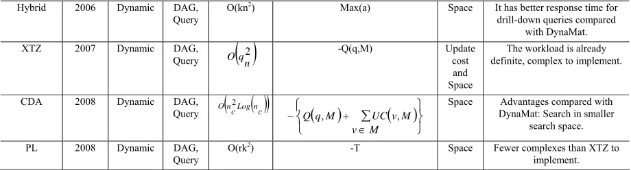
Hybrid 2006 Dynamic DAG, Query
O(kn2) Max(a) Space It has better response time for drill-down queries compared
with DynaMat.
XTZ 2007 Dynamic DAG,
Query O
( )
qn2-Q(q,M) Update cost
and Space
The workload is already definite, complex to implement.
CDA 2008 Dynamic DAG,
Query O
(
ncLog( )
nc)
2(
)
(
)
⎭ ⎬ ⎫ ⎩
⎨ ⎧
∑ ∈ + −
M v
M v UC M
q
Q , ,
Space Advantages compared with DynaMat: Search in smaller
search space.
PL 2008 Dynamic DAG,
Query
O(rk2) -T Space Fewer complexes than XTZ to implement.
based on each parameter. These algorithms have been extracted from well-known journals and conferences presented in ten recent years. We also present three reference algorithms (HRU, GM, and DynaMat). Details of these algorithms were presented in our previous work [15].
These algorithms are given below.
1. The algorithm presented by Harinarayan and et
al. (HRU Algorithm) [22].
2. The algorithm presented by Gupta and et al. (GM
Algorithm) [18]-[19].
3. Pick By Size Algorithm (PBS Algorithm) [37].
4. Polynomial Greedy Algorithm (PGA Algorithm)
[32].
5. View Relevance Driven Selection Algorithm
(VRDS Algorithm) [45].
6. Randomized Algorithm [24], [28].
7. The algorithm presented by Aouiche and et al.
(CSA Algorithm) [5], [31].
8. Mid Point Locating Algorithm (MPL Algorithm)
[23].
9. DynaMat Algorithm [25]-[26].
10. Dynamic Materialized View Management Based
on Predicates (DMP Algorithm) [13].
11. The algorithm presented by Zhang and et al.
(ZYK Algorithm) [49].
12. Hybrid Algorithm [35]-[36].
13. The algorithm presented by Gong and et al.
(CDA Algorithm) [17].
14. The Algorithm presented by Xu and et al. (XTZ
Algorithm) [47].
15. The algorithm presented by Phan and et al. (PL
Algorithm) [34].
The comparisons of these algorithms are presented in Table 2. This table contains 7 static algorithms, 7 dynamic algorithms, and a randomized algorithm which has static and dynamic versions. All of the algorithms are evaluated based on five parameters extracted from their evaluations according to their reports on the reference papers. These parameters are the type of algorithm, the type of their input, time complexity, benefit function, and constraining factors. Therefore, Table2 has 8 columns which are algorithm’s name, presentation year, 5 columns related to the parameters, and an analysis column containing algorithms’ analysis based on their techniques and the
results of accomplished experiments. Static algorithms, which use DAG (Directed Acyclic Graph) of cuboids as input, are compared with HRU algorithms and the other static algorithms are compared with the GM algorithm. Dynamic algorithms are compared with DynamMat. In the upper rows static algorithms and in the lower rows dynamic algorithms are presented. These two types have been ordered by time.
We can classify algorithms through various parameters. These classifications are listed below.
1. Algorithms classification based on their types:
Static algorithms, and Dynamic algorithms.
2. Algorithms classification based on input types:
algorithms which use and/or graph of input queries as input, algorithms which use DAG of cuboids as input, and algorithms which use input queries as input.
3. Algorithms classification based on constraining
factors: algorithms which are based on restricted space, algorithms which are based on restricted time to refresh materialized views, and algorithms which are based on the above-mentioned constraining factors.
4. Algorithms classification based on time
complexity: algorithms, which have exponential time complexity, and algorithms, which have polynomial time complexity.
5. Algorithms classification based on the
parameters required to calculate their benefit functions: the benefit function of algorithms is based on parameters which are: update frequency, query processing cost, update cost, query frequency, the space required to materialize a view, the number of queries which can be answered through a materialized view with improved response time.
6. Dynamic algorithms classification based on their
queries: algorithms with unknown input queries, and algorithms with known sequence of incoming queries.
5. THE TYPE OF APPLICATIONS IDENTIFICATION
The second step to select the suitable algorithm for view selection is the type of application identification. We define the data structure of the type of application identification process in the form of a function with inputs and outputs as:
CA v UC q s d q
AC
⎟
→⎠
⎞
⎜
⎝
⎛
, , , (2)In this function, AC is a function to specify application
type, and CA is an application with the specified type. In
this step, we should identify different parameters which are important to identify the type of applications. These parameters are the inputs of this function and extracted through investigation of data mining applications and decision support systems applications [20], [43] and are described as follows.
1. q: stands for query type in applications. In some
applications, the queries are known before arriving [14].
2. d: stands for the number of dimensions in
applications.
3. sq: stands for the type of sequence of statements.
In some applications, the sequence of statements is known and in other applications, they are unknown. Sequence of statements contains queries, updating, and their order of execution.
4. UCv: stands for view maintenance cost. Some
applications have limited time to update and refresh materialized views and in the others it is not an important issue. There are different algorithms for these two types.
Based on the value of the above parameters, the most suitable algorithm for view selection in different applications can be selected.
6. THE ROADMAP TO SELECT THE MOST SUITABLE VIEW
SELECTION ALGORITHM FOR APPLICATIONS
Creating roadmap as a third step is defined in this section. The roadmap is created based on two factors: the
parameters of applications, and the algorithms’ properties. The other factors such as data distribution is not directly affect the algorithm selection. These can be used as parameters in the state of preprocessing to achieve the roadmap.
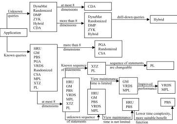
Fig.1 presents the proposed roadmap to select the suitable algorithm based on application parameters. The proposed roadmap is created based on 15 available algorithms and can be generalized. To add new algorithm to this roadmap, it is necessary to recognize the properties of each of them.
In this roadmap, the type of queries is first checked. If they are unknown, all of the dynamic algorithms except XTZ and PL algorithms should be used. Therefore, there are six choices: DynaMat, Randomized, CDA, Hybrid, DMP, and ZYK. Then, the number of dimensions in the application should be checked. If this number is at most 8, CDA is the most suitable algorithm because it searches in the smallest search space and selects suitable views in a reasonable time. If the number of dimensions is more than 8, other algorithms should be used. In this type, Hybrid algorithm is the best one when there are drill-down queries.
If the queries are known before arrival, all of the static algorithms, Randomized, XTZ, and PL algorithms can be used. If the number of dimensions is more than 8, fast algorithms such as PGA, CSA, or Randomized algorithms should be used.
If the queries of applications are known before their arrival and an application has at most 8 dimensions, HRU, GM, PBS, PGA, VRDS, CSA, MPL, PL, and XTZ algorithms can be used. If an application has known sequence of statements, XTZ and PL are more suitable algorithms. XTZ is more complex than PL to implement. If the order of queries’ execution is changeable, PL algorithm is more suitable than XTZ.
Figure 1: The roadmap to select the best suitable view selection algorithm.
Figure 2: The used path in the roadmap to select the view selection algorithm for the Sell application.
If 1) the queries of application are known, 2) an application has at most 8 dimensions, 3) the order of queries’ execution is unknown, and 4) the view maintenance cost is not important, HRU or PBS algorithms should be used. PBS has lower time complexity and more suitable benefit function. This algorithm is recommended in this situation.
The roadmap can be used to select the most suitable algorithm for each type of applications. For example, assume there are sale queries in a data warehouse system. It consists of five major dimensions: parts, suppliers, customers, times, items. Suppose that the orders of
queries’ execution are known. Whereas queries are known before arrival, HRU, GM, PBS, PGA, VRDS, Randomized, CSA, MPL, PL, and XTZ algorithms can be used. These queries have 5 dimensions, then HRU, GM, PBS, VRDS, MPL, PL, and XTZ algorithms are more suitable. As the order of queries’ execution is known, XTZ and PL algorithms are more suitable algorithms for this application. If the order of queries’ execution is changeable, PL is more suitable than XTZ. However, XTZ is more complex than PL to implement.
View maintenance time is not limited
Lower time complexity, more suitable benefit function
Improved performance View maintenance
time is limited
unknown sequence of statements
sequence of statements are changeable Known sequence
of statements
at most 8 dimensions
drill-down queries
more than 8 dimensions more than 8 dimensions
at most 8 dimensions
Known queries Unknown queries
DynaMat Randomized DMP ZYK Hybrid CDA
HRU GM PBS PGA VRDS Randomized CSA MPL XTZ PL Application
CDA DynaMat Randomized DMP ZYK Hybrid
Hybrid
PGA Randomized CSA
HRU GM PBS VRDS MPL XTZ PL
XTZ PL
HRU GM PBS VRDS MPL
GM VRDS MPL
HRU PBS
PL
VRDS MPL
PBS
View maintenance time is not limited
Lower time complexity, more suitable benefit function
Improved performance View maintenance
time is limited
unknown sequence of statements at most 8
dimensions Known queries
HRU GM PBS PGA VRDS Randomized CSA MPL XTZ PL Application
HRU GM PBS VRDS MPL XTZ PL
HRU GM PBS VRDS MPL
GM VRDS MPL
HRU PBS
VRDS MPL
7. TEST AND EVALUATION OF THE PROPOSED ROADMAP
In this section, sale database is introduced to test and evaluate the proposed roadmap. This database contains 5 main tables which are presented below.
Shop (shop_id int, name char(30), address char(120)) (2) Customer (customer_id int, nationality char(30), birthdate
date, address char(120)) (3)
Seller (seller_id int, name char(30), birthdate date) (4) Item (item_id int, name char(30), size char(30), producer cahr(30), type char(30)) (5) Sell (id int, selldate date, price int, customer_id int,
seller_id int, item_id int) (6)
Sell database contains the information about sells in 20 recent years from a chain store which contains 1000 branches in a country with 20 states. This shop has 10000 sellers and 1000000 customers which have 10 nationalities and ages between 20 and 80 years. Moreover, this shop has 10000 different items in 7 sizes and 10 types.
The input queries to this database are given in Appendix 2. The execution order of these queries is not definite. The Sell table is the main table of this database and has been contained in the “from clause” of all queries. These queries are divided in two groups:
1.Ten first queries require data extraction and
transformation to execute.
2.Ten last queries require join operation, data
extraction and transformation to execute.
Join operation is a time consuming operation. If sell
table has 2*107 records, 2.002*1026 records should be
joined to execute ten last queries. If views are created to execute these queries, these records should be joined again. If these views are materialized before query processing to create a data warehouse, join operations are removed during query processing leading to a query processing improvement.
Concerning the above analysis, as there are multidimensional aggregate queries, it should be created a data warehouse to improve the query response time [14]. The aggregate function of these queries is “sum” and dimensions are: Time, Item, Customer, Shop, and Seller. The huge amount of space is required to store the related cube without considering the hierarchies of dimensions
(2.103*1018 records). As the space is limited, the set of
more suitable views should be selected to materialize. Therefore, a suitable view selection algorithm should be used to select proper views. The proposed roadmap should be used to select the most suitable algorithm. Whereas there are predefined queries, HRU, GM, PBS, PGA, VRDS, Randomized, CSA, MPL, XTZ, and PL algorithms could be used. Since Sale data warehouse has 5 dimensions, HRU, GM, PBS, VRDS, MPL, XTZ, and PL algorithms are more suitable. As the order of queries execution is not predefined, HRU, GM, PBS, VRDS, and MPL algorithms can be used. If there is limited time to refresh views, VRDS and MPL algorithms should be
used; otherwise, the PBS algorithm is more suitable. The used path in the roadmap to select these algorithms is presented in Fig. 2.
The space required to materialize the views
corresponding input queries is 4.968*109 records. In this
paper, the equal space in average for each record is assumed. The performance of the PBS algorithm is considered with the assumption that the space allocated for the materialized views is 10 percent of the required space.
The PBS algorithm selects views in increasing size until the space limitation is reached. If this algorithm is executed, only the views related to the query8, query9, and query10 cannot be materialized. The ratio of the query processing cost in data warehouse (created through PBS algorithm) to the database could be calculated through formula 7. In this formula, the benefit of removing join operations and the pre-process to extract and transform some fields (such as customer age, seller age, and the state of a shop) are relinquished.
the ratio of the query processing cost
∑
∑
=i ic
i is (7)
In this formula, ci is the processing cost of the ith query
(qi) on the database and si is the processing cost of the ith
query (qi) on the data warehouse. The number of records
in each table, which is accessed to answer a query, has
direct effect on both ci and si. The numerator of this
formula is 4.28*108, and the denominator is 2.002*1026.
These two costs are incomparable. Therefore, the proposed roadmap causes high improvement in processing multidimensional aggregate queries.
If there is a limited time to refresh and maintain materialized views, MPL, or VRDS algorithms should be used and we reach to the similar results obtained through PBS algorithm.
8. CONCLUSIONS
Multidimensional aggregate queries are the main working units used in decision support systems. These queries are complex, and operate on huge amount of data. To improve query response time, the multidimensional structure to store data are needed. Data cube is the structure of the data warehouses to represent data sources in a multidimensional structure. Several view selection algorithms are available to materialize views to build efficient data warehouses. These algorithms have various parameters and are suitable for different applications. For each application, it should be selected the efficient one to have a quick query response.
the parameters to classify applications, and presented the roadmap to select the most suitable algorithm for view selection based on both these parameters and different types of algorithms. We tested and evaluated the proposed roadmap for a database and its queries as instance and calculated its improvement, and showed that this roadmap is suitable to select the most suitable algorithm for different applications.
9. APPENDIX
Appendix 1: List of Notation
a: the probability to access a materialized view. A: the smallest father of view v in materialized views. C: the number of clusters.
c(x): the actual benefit of materializing a view, when we have a set of materialized views, minus the cost of re-materialization.
C(v,M): the cost materialization a view v, when we have a
set M of materialized views.
d: the number of dimensions.
fq: the frequency of query q.
fuq: the frequency of the update statement.
fP: the frequency of the property P in input queries.
G: graph of input queries. h: the depth of local minimum.
i: the number of iterations in a genetic algorithm. k: the number of the selected views to materialize. l: the number of layers in the lattice of cuboids and is equal to d+1.
M: the set of materialized views.
m: the number of nodes in a graph of input queries. n: the number of nodes in a lattice of cuboids and is equal to 2d.
NC: the number of cuboids which can be used to calculate
a view v.
Nq: the number of queries that can be answered through v.
nc: the average number of views in clusters.
P: the total number of properties in all dimensions.
Q(q,M): the cost of answering query q through M.
qn: the number of input queries.
Rows(v): the number of rows in v.
r: the number of the materialized views which should be deleted.
s: the number of combinations of views to materialize. Sv: the size of view v.
SP: the space required to materialize the partitioned view
through property P.
T: the time required to execute all queries.
UC(v,M): the cost of updating view v when we have the
set M of materialized views.
Appendix 2: Input Queries to Sell Database
Select sum(price), year, item_id from Sell
group by year, item_id (1) Select sum(price), year, quarter, item_id
from Sell
group by year, quarter, item_id
where quarter=2 and item_id=40 (2)
Select sum(price), year, month, item_id, customer_age from Sell
group by year, month, item_id, customer_age
where month=1 and item_id=40 (3) Select sum(price), year, month, quarter, item_id from Sell
group by year, month, item_id (4)
Select sum(price), year, item_id, customer_age from Sell
group by year, item_id, customer_age (5)
Select sum(price), year, item_id, shop_id from Sell
group by year, item_id, shop_id (6) Select sum(price), item_id, seller_id
from Sell
group by item_id, seller_id (7) Select sum(price), year, quarter, month, item_id, shop_id from Sell
group by year, month, item_id, shop_id (8) Select sum(price), year, quarter, item_id, shop_id from Sell
group by year, quarter, item_id, shop_id
where quarter=2 (9) Select sum(price), year, item_id, seller_id
from Sell
group by year, item_id, seller_id (10) Select sum(price), year, month, type, region
from Sell,Item, Shop
group by year, month, type, region
where type=’clothes’ and month=12 (11) Select sum(price), type, customer_age
from Sell, Item, Customer group by type, customer_age
where type=’electric’ (12) Select sum(price), year, month, quarter, item_id, region from Sell, Shop
group by year, month, item_id, region (13)
Select sum(price), year, item_id, nationality from Sell, Customer
group by year, item_id, nationality (14) Select sum(price), year, month, quarter, type, shop_id from Sell, Item
group by year, month, type, shop_id (15) Select sum(price), year, month, type, seller_age from Sell, Item, Seller
group by year, month, type, seller_age (16) Select sum(price), size, customer_age, region
from Sell, Item, Customer, Shop
from Sell, Seller
group by year, month, item_id, seller_age (18) Select sum(price), year, month, size, customer_age from Sell, Item
group by year, month, size, customer_age (19) Select sum(price), year, quarter, size, region
from Sell, Shop, Item
group by year, quarter, size, region (20)
10. ACKNOWLEDGMENT
We would like to thank Professor Mohammad Bagher Menhaj for his helpful editorial comments.
This research has been supported partially by Education & Research Institute for ICT (ERICT).
11. REFERENCES
[1] Agrawal S., Chaudhuri S., Narasayya V.; “Automated Selection of
Materialized Views and Indexes for SQL Databases”, 26th
International Conference on Very Large Databases, Cairo, Egypt, pp. 496-505, 2000.
[2] Agrawal S., Chaudhuri S., Kollar L., Marathe A., Narasayya V., Syamala M.; “Database Tuning Advisor for Microsoft SQL Server
2005”, 30th VLDB Conference, Toronto, Canada, pp. 1110-1121,
2004.
[3] Agrawal S., Narasayya V., Yang B.; “Integrating Vertical and Horizontal Partitioning into Automated Physical Database
Design”, SIGMOD 2004, Paris, France, pp. 359-370, 2004.
[4] Aouiche K., Darmont J.; “Data mining-based materialized view
and index selection in data warehouses”, Journal of Intelligent
Information System (2009) 33:65–93, 2009.
[5] Aouiche K., Jouve P. E., Darmont J.; “Clustering-Based
Materialized View Selection in Data Warehouses”, 10th
East-European Conference on Advances in Databases and Information Systems (ADBIS06), Thessaloniki, Greece, 2006.
[6] Asgharzadeh Talebi Z., Chirkova R., Fathi Y., Stallmann M.;
“Exact and Inexact Methods for Selecting Views and Indexes for
OLAP Performance Improvement”, EDBT ’08, March 25-30,
2008, Nantes, France, pp. 311-322, 2008.
[7] Bellahsene Z., Marot P.; “Materializing a Set of Views: Dynamic
Strategies and Performance Evaluation”, 2000 International
Symposium on Database Engineering & Applications, IEEE , pp. 424-428, 2000.
[8] Chan G.K.Y., Li Q., Feng L.; “Design and Selection of Materialized Views in a Data Warehousing Environment: A Case
Study”, DOLAP99, Kansas City MO USA, pp. 42-47, 1999.
[9] Chaudhuri S., Narasayya V.; “An Efficient, Cost-Driven Index
Selection Tool for Microsoft SQL Server”, 23rd VLDB Conference
Athens, Greece, pp. 146-155, 1997.
[10] Chirkova R., Halevy A.Y., Suciu D.; “A formal perspective on the
view selection problem”, The VLDB Journal (2002) 11, pp. 216–
237, 2002.
[11] Chirkova R., Li C.; “Answering queries using materialized views
with minimum size”, The VLDB Journal (2006) 15(3) pp. 191–210,
2006.
[12] Chirkova R., Li C.; “Materializing Views with Minimal Size to
Answer Queries”, PODS’03, San Diego, CA, pp. 38-48, 2003.
[13] Choi C. H., Yu J. X., Lu H.; “Dynamic Materialized View
Management Based on Predicates”, Springer, APWeb 2003,
LNCS, pp. 583-594, 2003.
[14] Daneshpour N., Abdollahzadeh Barfourosh A.; “AUT-QPM: The New Framework to Query Evaluation for Data Warehouse Creation”, Iranian Journal of Electrical and Computer Engineering Vol. 6, N. 1, pp. 35-45, 2008.
[15] Daneshpour N., Abdollahzadeh Barfourosh A.; “View Selection
Algorithms to Build Data Warehouse”, Technical Report: AIS Lab,
IT & Computer Engineering Department, Amirkabir University of Technology, CE/ TR.DS/ 86/ 01, http://ceit.aut.ac.ir/~daneshpour/Publications.htm, 2008.
[16] Ezeife C.I.; “Selecting and materializing horizontally partitioned
warehouse Views”, Data & Knowledge Engineering 36, pp.
185-210, 2001.
[17] Gong A., Zhao W.; “Clustering-based Dynamic Materialized View
Selection Algorithm”, Fifth International Conference on Fuzzy
Systems and Knowledge Discovery, IEEE, pp. 391-395, 2008. [18] Gupta H.; “Selection of Views to Materialize in a Data
Warehouse”, In Intl. Conf. On Database Theory, Delphi, Greece,
pp. 98-112, 1997.
[19] Gupta H., Mumick I.S.; “Selection of Views to Materialize in a
Data Warehouse”. IEEE Trans. Knowledge and Data Engineering,
Volume 17, Issue 1, pp. 24 – 43, 2005.
[20] Han J., Kamber M.; Data Mining: Concepts and Techniques, Second Edition, Morgan Kaufmann Publishers, 2006.
[21] Hanusse N., Maabout S., Tofan R.; “A view selection algorithm
with performance guarantee”, EDBT 2009, March 24–26, 2009,
Saint Petersburg, Russia. pp. 946-957, 2009.
[22] Harinarayan V., Rajaraman A., Ullman J.D.; “Implementing Data
Cubes Efficiently”, SIGMOD'96 6/96 Montreal, Canada, pp.
205-216, 1996.
[23] Hung M.C., Huang M.L., Yang D.L., Hsueh N.L.; “Efficient approaches for materialized views selection in a data warehouse”,
ELSEVIER Trans. Information Sciences 177, pp. 1333–1348, 2007.
[24] Kalnis P., Mamoulis N., Papadias D.; “View Selection Using
Randomized Search”, ELSEVIER Trans. Data & Knowledge
Engineering, vol. 42, pp. 89–111, 2002.
[25] Kotidis Y., Roussopoulos N.; “A Case for Dynamic View
Management”, ACM Transactions on Database Systems, Vol. 26,
No. 4, pp. 388–423, 2001.
[26] Kotidis Y., Roussopoulos N.; “DynaMat: A Dynamic View
Management System for Data Warehouses”, SIGMOD’99
Philadelphia PA, pp. 371-382, 1999.
[27] Lawrence M.; “Multiobjective Genetic Algorithms for Materialized
View Selection in OLAP Data Warehouses”, GECCO’06, Seattle,
Washington, USA, pp. 699-706, 2006.
[28] Lawrence M., Rau-Chaplin A.; “Dynamic View Selection for
OLAP”, DaWak 2006, LNCS 4081, Springer, pp. 34-44, 2006.
[29] Liang W., Wang H., Orlowska M.E.; “Materialized view selection
under the maintenance time constraint”, Data & Knowledge
Engineering 37, pp. 203-216, 2001.
[30] Liu Y. C., Hsu P. Y., Sheen G. J., Ku S., Chang K. W.;
“Simultaneous determination of view selection and update policy with stochastic query and response time constraints”, Information Sciences 178 (2008) 3491–3509, 2008.
[31] Mahboudi H., Aouiche K., Darmon J.; “Materialized View
Selection by Query Clustering in XML Data Warehouses”, 4th
International Multiconference on Computer Science and Information Technology (STIC 06), Amman, Jordan, 2006. [32] Nadeau T.P., Teorey T.J.; “Achieving Scalability in OLAP
Materialized View Selection”, DOLAP ’02, McLean, Virginia,
USA, pp. 28-34, 2002.
[33] Neapolitan R. “Fundamentals of Algorithms Using C++
Pseudocode”, Jones and Bartlett Publishers, Inc.; 3rd edition,
2003.
[34] Phan T., Li W. S.; “Dynamic Materialization of Query Views for
Data Warehouse Workloads”, ICDE 2008, IEEE, pp. 436-445,
2008.
[35] Ramachandran K., Shah B., Raghavan V.; “Access Pattern-Based
Dynamin Pre-fetching of Views in an OLAP System”, International
Conference on Enterprise Information Systems, 2005.
[36] Shah B., Ramachandran K., Raghavan V.; “A Hybrid Approach for
Data Warehouse View Selection”, International Journal of Data
Warehousing and Mining, Vol. 2, Issue 2, 2006.
[37] Shukla A., Deshpande P.M., Naughton J.F.; “Materialized View
Selection for Multidimensional Datasets”, VLDB, Morgan
Kaufmann, pp. 488-499, 1998.
[38] Souza M.F.D., Sampaio M.C.; “Efficient Materialization and Use
of Views in Data Warehouses”, SIGMOD Record, Vol. 28, No. 1,
[39] Theodoratos D., Sellis T.; “Designing Data Warehouses”, Data & Knowledge Engineering 31, pp. 279-301, 1999.
[40] Theodoratos D., Bouzeghoub M.; “A General Framework for the View Selection Problem for Data Warehouse Design and
Evolution”, DOLAP '00 11/00 McLean, VA, USA, pp. 1-8, 2000.
[41] Theodoratos D., Ligoudistianos S., Sellis T.; “View Selection for
Designing the Global Data Warehouse”, Data & Knowledge
Engineering 39, pp. 219-240, 2001.
[42] Theodoratos D., Xu W.; “Constructing Search Spaces for
Materialized View Selection”, DOLAP’04, Washington, DC, USA,
pp. 112-121, 2004.
[43] Turban E., Aronson J.E., Liang T.P., Sharda R.; Decision Support
and Business Intelligence Systems, 8nd Edition, Prentice Hall,
2006.
[44] Uchiyama H., Runapongsa K., Teorey T.J.; “A Progressive View
Materialization Algorithm”, DOLAP99, Kansas City MO USA,
pp. 36-41, 1999.
[45] Valluri S.R., Vadapalli S., Karlapalem K.; “View Relevance Driven
Materialized View Selection in Data Warehousing Environment”,
ADC2002, vol. 5, pp. 187-196, 2002.
[46] Xu W., Theodoratos D., Zuzarte C.; “Computing Closest Common
Subexpressions for View Selection Problems”, DOLAP’06,
Arlington, Virginia, USA, pp. 75-82, 2006.
[47] Xu W., Theodoratos D., Zuzarte C.; “A Dynamic View Materialization Scheme for Sequences of Query and Update
Statements”, DaWaK 2007, LNCS 4654, pp. 55-65, 2007.
[48] Yu J.X., Yao X., Choi C.H., Goa G.; “Materialized View Selection
as Constrained Evolutionary Optimization”, IEEE Transactions on
Systems, Man and Cybernetics-Part C: Applications and Reviews, vol. 33, no. 4, pp. 458-467, 2003.
[49] Zhang C., Yang J., Kalapalem K.; “Dynamic Materialized View
Selection in Data Warehouse Environment”, Informatica