Assessment of Cost Effectiveness of a Firm Using Multiple Cost Oriented DEA and Validation with MPSS based DEA

593

Available online at http://ijdea.srbiau.ac.ir

Int. J. Data Envelopment Analysis (ISSN 2345-458X)

Research Article

Assessment of Cost Effectiveness of a Firm Using

Multiple Cost Oriented DEA and Validation with

MPSS based DEA

Subhadip.Sarkar

(a) Department of Management Studies, NIT Durgapur, West Bengal, India.

Received 09 December 2014, Revised 07 February 2015, Accepted 27 February 2015 Abstract

Data Envelopment Analysis (DEA) is a nonparametric tool for discriminating the best performers from a number of homogenous Decision Making Units (DMU). Cost oriented DEA models identify those best DMUs which run cost efficient process. This paper validates the outcome derived from the Ideal Frontier (mentioned in Sarkar. S (2014)) derived from non-central Principal Component Analysis and a slack based optimization model to identify the cost efficient DMUs. Instead of offering real cost of each resource, the proposed model minimizes the projection of inputs along the direction of first Eigenvector of specific covariance matrix from each allocated outputs. These essential directions vectors represent various "combined consumption (cost)" for the production of outputs. A Multi-Objective Fuzzy Goal Programming model is applied here to solve this multi-objective problem. Superiority is judged on the basis of higher value of a cost oriented performance ratio. A case study of six schools is incorporated here to identify the superior cost efficient school and also to visualize gaps in their performances.

Keywords: Data Envelopment Analysis, non-central Principal Component Analysis, Non-Stochastic

DEA, Frontier Function.

*_{Corresponding author: [email protected]}

594 1. Introduction

The journey of Data envelopment analysis (DEA), as proposed by Charnes et al. (1978) [3] (the CCR model), commenced from the dissertation of Rhodes when the performance of students from participating and not participating schools were compared using a nonlinear model and an equivalent data-oriented, linear programming-based, nonparametric approach. A DMU is called an efficient performer if it uses fewer quantities of each input to generate the same set of outputs or produces more outputs from the same set of input resources than its rivals. Thus, it makes a place in a production possibility set. Later on, the assumption of constant return on scale (CRS), was extended by Banker et al. (1984) [1]. The renowned BCC model of these researchers was able to administer variable scaling techniques. As a result, weak efficient and strong efficient DMUs, MPSS (most productive scale size) and, SE (scale efficiency) became prevalent. To estimate the CRS frontier function, the regression approach was modified by Winsten (1957) [15] by using a corrected ordinary regression technique. It enabled the detection of CRS efficient DMU instead of classifying them into below average, average and above average units (Cooper, W. W and L. M. Seiford (2011) [4]). Later on, the DEA estimators were found statistically consistent (Banker and Maindiratta (1992) [2]). The detailed methodology of the frontier function

estimation was done by Greene. W. H (1980) [6] on a generalized form proposed by Aigner and Chu (1968). The exploration of stochastic DEA (SDEA) has proven to be highly effective for adapting this approach to abrupt changes. The experiment on “Program follow Through and Non-follow Through” school sites (originally considered by Charnes et al. (1981)) was revisited by Land et al. (1993) [8] who, instead of taking average values for inputs and outputs, suggested a deterministic equivalent of the chance constrained model by assuming normally distributed output variables which were conditional on inputs. In an efficiency evaluation of the research activities

in economic departments at Danish

Universities, Olesen and Petersen (1995) [9] developed a chance constrained programming model while distinguishing two reasons (true inefficiency and random disturbance) to remain inefficient.

595 producing highly correlated weighted scores with the DEA productivity indexes of the DMUs.

In this paper, the performances of a set of DMUs are assessed by means of MOLP cost oriented DEA model. The reason of adopting this model is to identify those CCR efficient DMUs which are able to minimize the "combined consumption" for all possible outputs. The direction of the "combined consumption" is the first Eigenvector derived from non-central PCA on specific covariance matrix and explains a comprehensive portion of the total variation from the origin. This leads to a minimization of a number of cost functions (equivalent to the number of outputs in the given problem). A Fuzzy Goal programming model is applied here to solve this multi-objective problem. The outcome of this model is validated with the outputs of an MPSS based CRS frontier function described in Sarkar. S (2014) [12]. Both models show a substantial association in this regard.

2. Definitions and Theorems:

2.1. Data Envelopment Analysis with CCR Model:

From an assumption of constant returns to scale, Charnes et al (1978) [3] found proportional changes in weighted output that derive from the alterations in weighted inputs. The algebraic models of CRS (constant return to scale) for c DMUs (each of which consumes v inputs given by the matrix to

generate m outputs given by a matrix ) are as follows:

Primal form Dual form

(∑ )

Subjected to: ∑ ∑ ∑

For any DMU r

Subjected to: ∑

For any jth input

∑

2.2. Solution of MOLP using Fuzzy Goal Programming:

Zimmermann, H. J., (1978) [16] has shown that even in presence of crisp type of constraints and conflicting objective functions, upper and lower goals can be set for each objective function while optimizing only one objective function. A fuzzy membership function is created and maximized later on, based on the nature of the assigned objective functions, to derive the solutions for the decision variables at a satisfactory level of the membership function.

2.3. A CCR-Efficient Unit:

596 involve at least one DMU (known as a peer group) within the given set that manages to yield weighted outputs that are equivalent to its weighted inputs. The set of peer groups is specified as follows:

{ ∑ ∑ }

2.4. Production Possibility Set:

The set of all technically feasible

combinations of inputs and outputs,

representing the technology of a firm.

According to Cooper et al, (2011) [5], in case of a CCR model, any production possibility set, is defined as follows:

(A1) If an activity belongs to P, then

the activity belongs to P for any

positive scalar t.

(A2) For an activity in P, any

semi-positive activity with and is included in P. That is,

any activity with input no less than in any component and with output no greater than in any component is feasible.

(A3) the nonnegative combination of the DMUs in the set J as:

{( |

∑

∑

)}

2.5. Principal Component Analysis:

PCA can be defined as the orthogonal projection of the data onto a lower dimensional linear space, known as the principal subspace, such that the variance of the projected data is maximized in the

subspace. According to Rencher (2002) [11], Principal component analysis deals with a single sample of n observation vectors y1, y2,...

, yn that form an ellipsoidal swarm of points in a p-dimensional space. If the variables y1, y2,... , yp in y are correlated, the natural axes of the swarm of points become identical to with the axes of the ellipsoid having an origin at the mean vector (y*) of y1, y2,... , yn. The resulting natural axes of the ellipsoid yield the new uncorrelated variables called (principal components). These resulting axes will be similar to the Eigenvectors ( ) derived from the covariance matrix (or the

correlation matrix ( ) of the observed

variables which also minimizes the mean squared distance between the data points and their projections (shown below).

2.6. Specific Consumption Matrix T and Specific Covariance Matrix S:

Under the conditions of m = 1 and v < c in a primal-model of the DEA (CCR), there exist a positive definite covariance matrix S derived from the origin (having with a non-zero determinant) with dimensions of (v x v) that can be defined as follows:

 

 

(

2

)

,

0

rj ri r ij cxv

r ij r

ij vxv

ij r T r r

y

R

t

where

t

T

and

s

where

s

T

T

S









597

)

3

(

...

...

]

[

];

[









































































j

i

y

R

y

R

j

i

y

R

s

t

t

t

T

where

T

T

T

T

tij is known as the specific usage (SU) of the i th

input of the rth DMU.

2.7.A Non-central PCA and its Application on Specific Covariance Matrix Sv:

To observe the mutually independent underlying characteristics of resource utilization the specific consumption matrix is projected on a unit vector so that the directions of maximum variance (from the origin vector and not from their mean vector) can be explored. This leads to the following optimization problem to be solved:

The optimal solution of this problem gives rise to Eigenvectors of Sv which are orthogonal to each other.

2.8. Economic Interpretation of Principal Components of the Matrix Sv:

Being a square matrix of size (v x v), Sv, has v number of Eigenvectors (and Eigen values). These vectors carry significant information about the usage of all ingredients. Other than the first vector none of the remaining ones

assume all positive elements (shown in the appendix 1 and appendix 2). The first Eigenvector acknowledges the cost consciousness of a firm as less projected value on this vector implies the lower combined consumption of inputs. The reason of calling it “cost” or “combined spending” is that, the firm in view of acquiring future benefits would like to concentrate on the current collective expenditure. Remaining dimensions (which reflect unique capacity of a firm) are indeed essential to gain various competitive advantages. Each of these vectors has its own priority level (equivalent to the corresponding Eigen value) set by the Industry. Baring this, they contain one negative element which is indicative of the worth of a particular resource over the rest for reducing the cost due to that dimension. Therefore, the firm has to be more decisive in managing the cost and the right dimension to sustain in the market. Therefore, the proposed model lies on the balance between (i) reduction of “cost” (which focuses on decreasing the utilization of resources) and (ii) reduction of cost from the remaining dimensions (by manipulating proper resources).

2.9. Proposed Multi-Objective Cost oriented DEA Model:

598 and number of outputs, there will be

number of traits (shown below with their priority levels.

E

ig

en

v

ec

to

r

Prio

rity

lev

el

Ou

tp

u

t 1

Ou

tp

u

t 2

---

Ou

tp

u

t m

Eigenvector

1 1 (top) E11 E12 - E1m Eigenvector

2 2 E21 E22 - E2m

-- Eij

Eigenvector

v

v

(least) Ev1 Ev2 - Evm Output Weight w1 _{w2 - wm} The first Eigenvector of each output refers to a cost and does explain a comprehensive amount of variation of specific covariance matrix. It is therefore necessary for a firm to minimize all of them to stand tall in regard to operational efficiency. However, neither the priority level of the outputs nor the weights are available. So, assuming equal priority for each output, a multiple cost oriented fuzzy goal programming is applied here.

Minimize objective function: ∑ Subjected to:

∑

For any jth input

∑

∑

Fuzzy Multi-Objective Programming originated by Zimmermann (1978) [16] is used for the above problem to find an optimal goal from a payoff matrix.

2.9.1. Cost Oriented Efficiency Measure: The cost oriented efficiency of any rth DMU is derived from the ratio given as:

(∑

∑ )

where, is the amount of ith resource used

by any rth DMU and is the optimal solution derived from the above model.

2.10. Definition of Inefficiency Error:

2.10.1. Inefficiency Errorin case of a Single Output:

The predicted amount of any rth output from any jth DMU, can be given by the dot product of the resource vector ( ) of the same DMU and the Eigen vector of the first principal component of a specific consumption matrix

which is derived from any rth output:

Thus, error ( ) on any rth output made by

any jth DMU can be determined by subtracting the observed output ( ) from the

predicted output given by .

( )

2.10.2. Inefficiency Error in case of a Multiple Outputs:

599

∑ ∑ (

) ∑

Here, ∑ ( ) and

_{∑ (}

)

, are the indicators

of the performance expected and actual performance from the jth DMU respectively. The unknown value of is determined by using the following LPP.

∑

∑ where,

2.11. Technical Efficiency or Performance Index:

The performance index of any jth DMU is given by the ratio of actual performance and expected performance as follows:

2.12. PCA Measure of Efficiency for DMUs:

If T = [tij], for{tij (> 0)}, is the specific consumption matrix consisting of elements tij, which represent the specific consumption of the ith type of input (for i = 1, 2…v) by the rth DMU (for r = 1, 2…c) then the PCA measure of efficiency for any DMU r is given by [min (T.U)/ (TJ.U)], where U is the eigenvector that directs the major axis of the embedded PCA and TJ is the specific consumption vector of the rth DMU. This Eigenvector describes the direction of maximum variation in case of a specific consumption under a particular type of output. The magnitude of projection taken in

this direction represents the keenness toward the production of the same output. A DMU is considered as keen to towards an output if the value of the projection is less.

2.12. Axiomatic Definition of the MPSS Frontier:

i) According to Starrett (Ray, S. C. 2004 [10]), any MPSS based transformation function can be represented as which has a ( ) ratio of 1. With an assumption of an explicit form of this function, is used here instead. The differential form of this model is displayed as follows:

∑ (

)

( ) (

)

∑ (

)

(

)

( )

( )

∑ (

)

( ) ∑ (

)

The later relationship of can be made if

becomes a linear function of all individual outputs, . This proposition is also valid due to the following equivalence and for a convex combination.

∑

∑

600

PCA efficient (and thus strongly efficient) in

each arena of output (efficient in all outputs).

iii) Basic elements within the set: If

is an element in this pseudo Production Possibility set, then, the pairs of

will also be contained by the same set for the conditions of

iv) Members on the frontier: If

is an efficient combination according to the

PCA, then, for any non-negative value t, the

pair of will be on the same plane.

v) Unlike CCR model the proposed

model assumes that any member in the

production possibility set should abide by the

following relation:

{ ∑

∑

}

is the maximum amount of any jth output for any rth DMU using the proposed model. The set is comprised with those DMUs which are

PCA efficient in each output. If such ultimate

performer is not present in the dataset then

will become a null set. In that case, it will not contain any technically feasible

combinations of inputs and outputs.

The predicted value of any output from all possible inputs is determined from a PCA based linear function. This production function satisfies the following postulates:

(P1) g(R) is monotonic in R. Since

( ) ( ) ,

then for and the

inequality of ( ) has to be true.

(P2) g(R) is concave. Hence, if

and

then

This property is also followed by the above proposed function (shown below).

(P3) For each observation, ,

( ) . Owing

to the relationship of the stated

relationship can be proved. ( )

.

3. A Mathematical Example

601 Table 1: Data

Schools Input 1 (I1)

Input 2 (I2)

Output 1 (O1)

Output 2 (O2)

A 8939 64.3 25.2 223

B 8625 99 28.2 287

C 10813 99.6 29.4 317

D 10638 96 26.4 291

E 6240 96.2 27.2 295

F 4719 79.9 25.5 222

Table 2 and Table 3 contain the outputs of CCR DEA. Scores shown in Table 2 clearly discriminates the inefficient schools B, C and D from the efficient schools A, E and F.

Table 2: CCR-DEA OUTPUT Productivity Value Productivity Value SCORE( A) 1 SCORE( D) 0.9143 SCORE( B) 0.9096 SCORE(E) 1 SCORE( C) 0.9635 SCORE( F) 1 The weight vector defined by (u*, q*) for each school is displayed in Table 3.

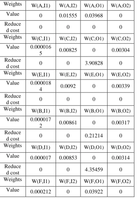
Table 3: Values of Input and Output Weights Weights _{W(A,I1) W(A,I2) W(A,O1) W(A,O2)}

Value _{0 0.01555 0.03968 0}

Reduce

d cost 0 0 0 0

Weights _{W(C,I1) W(C,I2) W(C,O1) W(C,O2)}

Value 0.000016

5 0.00825 0 0.00304 Reduce

d cost 0 0 3.90828 0 Weights _{W(E,I1) W(E,I2) W(E,O1) W(E,O2)}

Value 0.000018

4 0.0092 0 0.00339 Reduce

d cost 0 0 0 0

Weights _{W(B,I1) W(B,I2) W(B,O1) W(B,O2)}

Value 0.000017

2 0.00861 0 0.00317 Reduce

d cost 0 0 0.21214 0 Weights _{W(D,I1) W(D,I2) W(D,O1) W(D,O2)}

Value _{0.000017 0.00853 0 0.00314}

Reduce

d cost 0 0 4.35459 0 Weights _{W(F,I1) W(F,I2) W(F,O1) W(F,O2)}

Value _{0.000212 0 0.03922 0}

Reduce

d cost 0 0 0 0

The weight vector for any school is represented as W (name of the school, input/output). Although, efficient schools like A, E and F have weight vectors along with few zeroes, but the reduced cost in each cases remain absolutely zeroes (which is a must be condition for becoming efficient). The specific consumption patterns, in table 6, show that A assumes minimum value in input 2 under both outputs. Thus, it can be counted under the list of efficient DMUs. It also explains the reason that E and F achieve minimum specific consumption scores in input 1 under output 2 and in input 2 under output 1 respectively. The covariance matrix, Eigenvalues and Eigenvectors, pertaining to the embedded PCA, are shown in Table 7.

Table 4: Specific Consumption Matrix of Two Outputs Schools I1/O1 I2/O1

A 354.7222222 2.551587302

B 305.8510638 3.510638298 C 367.7891156 3.387755102 D 402.9545455 3.636363636 E 229.4117647 3.536764706 F 185.0588235 3.133333333 Schools I1/O2 I2/O2

A 40.08520179 0.288340807

602 These Eigenvectors assume largest degree of explanation (>90%) and reflects the usual practice of schools. First input has a higher impact than the second. Table 7 is important for the derivation of the expected amount of outputs. These MPSS based CRS frontiers, for each output, are shown below.

Spending has higher impact on both outputs than the later one. An efficient school must produce output according to these equations.

3.1. Proposed Multi-Objective Cost

Oriented Model:

As stated before in the definition 2.9, the original cost oriented DEA model will be treated with two objective functions. Both functions are to be minimized under the condition of CCR approach. This step is adopted to make a comparison between MPSS based DEA which itself is a CCR type of frontier. The final linear model is shown below:

min=z1; min=z2;

z1= 0.999949298*x1+0.010069824*x2; z2=0.9999*x1+0.01*x2;

8939*L1+8625*L2+10813*L3+10638*L4+6240* L5+4719*L6<=x1;

64.3*L1+99*L2+99.6*L3+96*L4+96.2*L5+79.9* L6<=x2;

25.2*L1+28.2*L2+29.4*L3+26.4*L4+27.2*L5+25 .5*L6>=25.2;

223*L1+287*L2+317*L3+291*L4+295*L5+222* L6>=223;

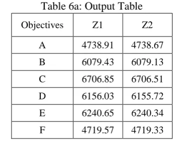
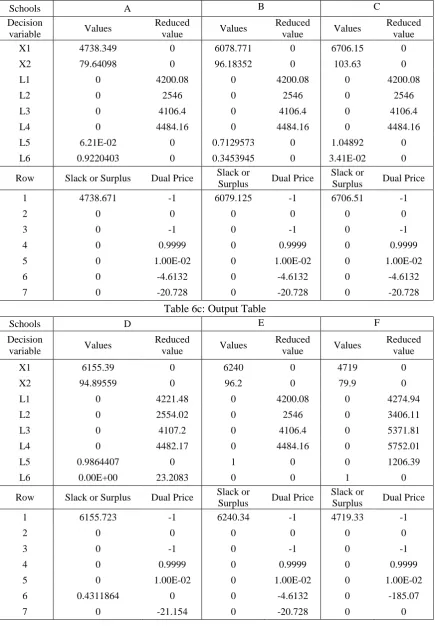
This optimization problem contains two non-conflicting objective functions. Thus, the solution technique of MOLP using a fuzzy goal programming does not create upper and lower limits for each individual objective function. This also prohibits the requirement of setting fuzzy goals and the maximization of the fuzzy membership function. The resulting values of the decision variables are shown below (Table 6a, Table 6b and Table 6c):

Table 6a: Output Table

Objectives Z1 Z2

A 4738.91 4738.67 B 6079.43 6079.13 C 6706.85 6706.51 D 6156.03 6155.72 E 6240.65 6240.34 F 4719.57 4719.33 It can be observed that apart from school E and F other schools are cost inefficient. Each one of them is dominated by a hypothetical school composed by E and F. It can also be shown that school C can become efficient when a variable return to scale is assumed. Table 5: The Eigenvalue and Eigenvector of the Covariance Matrix

Contents From Output 1 From Output 2

S Matrix 603890.4534 6081.332298 5909.2 59.2503 6081.332298 65.86168651 59.25 0.6455

Eigen-value 603951.6945 38.22645

Eigenvector 0.999949298 0.010069824

603

Table 6b: Output Table

Schools A B C

Decision

variable Values

Reduced

value Values

Reduced

value Values

Reduced value

X1 4738.349 0 6078.771 0 6706.15 0

X2 79.64098 0 96.18352 0 103.63 0

L1 0 4200.08 0 4200.08 0 4200.08

L2 0 2546 0 2546 0 2546

L3 0 4106.4 0 4106.4 0 4106.4

L4 0 4484.16 0 4484.16 0 4484.16

L5 6.21E-02 0 0.7129573 0 1.04892 0

L6 0.9220403 0 0.3453945 0 3.41E-02 0

Row Slack or Surplus Dual Price Slack or

Surplus Dual Price

Slack or

Surplus Dual Price

1 4738.671 -1 6079.125 -1 6706.51 -1

2 0 0 0 0 0 0

3 0 -1 0 -1 0 -1

4 0 0.9999 0 0.9999 0 0.9999

5 0 1.00E-02 0 1.00E-02 0 1.00E-02

6 0 -4.6132 0 -4.6132 0 -4.6132

7 0 -20.728 0 -20.728 0 -20.728

Table 6c: Output Table

Schools D E F

Decision

variable Values

Reduced

value Values

Reduced

value Values

Reduced value

X1 6155.39 0 6240 0 4719 0

X2 94.89559 0 96.2 0 79.9 0

L1 0 4221.48 0 4200.08 0 4274.94

L2 0 2554.02 0 2546 0 3406.11

L3 0 4107.2 0 4106.4 0 5371.81

L4 0 4482.17 0 4484.16 0 5752.01

L5 0.9864407 0 1 0 0 1206.39

L6 0.00E+00 23.2083 0 0 1 0

Row Slack or Surplus Dual Price Slack or

Surplus Dual Price

Slack or

Surplus Dual Price

1 6155.723 -1 6240.34 -1 4719.33 -1

2 0 0 0 0 0 0

3 0 -1 0 -1 0 -1

4 0 0.9999 0 0.9999 0 0.9999

5 0 1.00E-02 0 1.00E-02 0 1.00E-02

6 0.4311864 0 0 -4.6132 0 -185.07

604 Using the outputs of these tables the cost efficiency scores is derived (shown below in Table 7). On the contrary, being a CCR efficient School, A, does not have any significant role to play here, as it does not possess the needed efficiency score.

Table 7: Efficiency Measurement of Schools

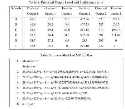
3.2. MPSS Based DEA model: Inefficiency creeps in if any deviation exists among the

observed output and the derived output. Table 8 shows the magnitude of inefficiency errors for each DMU in each output. The important aspect of this table is that school A, which has been considered as an efficient DMU, is scoring errors on both occasions. However, E and F are able to keep their errors very close to zero and hence can be counted under the list of efficient DMUs. Table 9 displays the MPSS based optimization model for problem considered above. The output of this LPP (shown in Table 10) depicts the proportions for mixing two scores. Three constraints which are considered for first three schools yield positive slack values are unable to reach up to the desired level of output. Efficiency Rank

A 0.53029 6

B 0.70482 3

C 0.62023 4

D 0.57866 5

E 1 2

F 1 1

Table 8: Predicted Output Level and Inefficiency error Schools Predicted

Output 1

Observed Output 1

Error in output 1

Predicted Output 2

Observed Output 2

Error in output 2

A 48.3 25.2 23.1 422.56 223 199.6

B 46.6 28.2 18.4 407.73 287 120.7

C 58.4 29.4 29.0 511.15 317 194.16

D 57.5 26.4 31.1 502.88 291 211.89

E 33.7 27.2 6.5 295 295 0

F 25.5 25.5 0 223.10 222 1.1

Table 9: Linear Model of MPSS DEA 1. Maximize S;

Subject to:

2. 25.2*a1+223*a2+S<= a1*48.2988238265909+a2*422.562114693711; 3. 28.2*a1+287*a2+ S<= a1*46.6042432434978+a2*407.736304094862; 4. 29.4*a1+317*a2+ S<= a1*58.4255279303645+a2*511.159703649781; 5. 26.4*a1+291*a2+ S<= a1*57.4798480100451+a2*502.886038920934; 6. 27.2*a1+295*a2+ S<= a1*33.718493954692+a2*295;

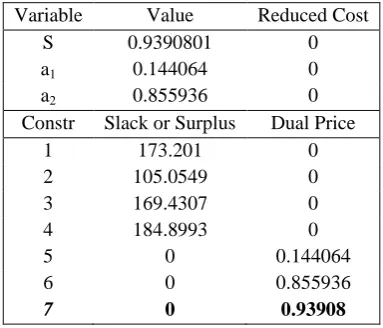
605 Table 10: Output of MPSS based DEA

Variable Value Reduced Cost

S 0.9390801 0

a1 0.144064 0

a2 0.855936 0

Constr Slack or Surplus Dual Price

1 173.201 0

2 105.0549 0

3 169.4307 0

4 184.8993 0

5 0 0.144064

6 0 0.855936

7 0 0.93908

The condition of the remaining last two schools is somewhat better in this regard. Though, the school F gets higher importance in this table and Table 11 clarifies its position from the column of Ranking. It ranks 2nd among others due to the ability of its students in the domain of language group. Having a positive dual price and first rank among the competitors, school E, sets a bench mark in the arena of science group. An extended output oriented CCR model is applied here for resolving the issue of contradictions stated before. The spearman’s correlation among the efficiency scores provides a strong association among these two methods.

4. Conclusion:

The proposed MOLP cost oriented DEA model is presented here to cite a proof of an existence of an Ideal Cost frontier originating from an MPSS based DEA (referred in Sarkar. S (2014) [12]). The former model has mentioned that it is not necessary for a CCR efficient DMU to remain cost competent. In the present problem school A is an example of that scenario. The proposed model, in this paper, has also supported this proposition. However, the former model has taken more rigorous attempt to measure the errors in terms of output production which could had been produced by an Ultimate producer. Apart from this, the magnitudes of these efficiency scores are greater than or equal to the proposed model than whatever is seen in Table 11. The reason of this difference can be realized by the fact that the proposed model is based on a pessimistic view which locates the MPSS frontier through points where the model maximizes the minimum error. Thus, the performance measured from this plane will always be less than whatever is found in case of new model.

Table 11: Combined Error

Schools

Error in output 1 (weight = 0.144)

Error in output 2 (weigh = 0.856)

Combined Error

Performance

ratio Ranking

A 23.1 199.6 174.15 0.52762 6

B 18.4 120.7 106.00 0.702023 3

C 29.0 194.16 170.38 0.617952 4

D 31.1 211.89 185.85 0.576408 5

E 6.5 0 0.9387 0.996353 1

F 0 1.1 0.9391 0.995175 2

606 Appendix 1: The Highest Eigenvalue of a Positive Definite Matrix that contains entirely positive elements will always be greater than the highest diagonal element of that matrix

Let A be a positive definite matrix with all non-negative elements, and let x be the eigenvector corresponding to the Eigenvalue, γ, then, from the definition of an Eigenvalue,

| | must hold:

| | [

]

(A1)

Thus, the linearized form of the first (n - 1) rows and n columns are as follows:

This can also be expressed as follows:

[ ] [

] [ ] (A2)

The first set of linear equation represents

which essentially

refers to two conditions;

As a

result, it can be interpreted that any ith element of an Eigenvector will be positive if the corresponding Eigen value is more than the ith diagonal element. Therefore, if an Eigenvector contains all positive elements then the relationship must

be true.

If another Eigenvector (which is orthogonal to ) is considered with a negative element . Then, the following equations will exist.

[ ] [

] [

]

[ ]

However, this will violate the condition

. Thus, an

Eigenvector with all positive elements can be generated only from the largest Eigen value. The second equation is given as

. Using the first

equation the following expression can be established.

( )

(A5) For the largest Eigen value, must

be true. The Eigenvector, corresponding to it, will necessarily make to happen and as a result it will also impose a positive definiteness to the matrix (as ).

References

[1] Banker, R. D., Charnes, A., Cooper, W. W. (1984). Some models for estimating technical and scale inefficiencies in data envelopment analysis. Management Science, 30(9), 1078-1092.

607 [3] Charnes, A., Cooper, W. W., & Rhodes, E. (1978). Measuring the efficiency of decision making units. European Journal of Operational Research, 2, 429-444.

[4] Cooper. W. W., Seiford. M. L., (2011) Hand Book on Data Envelopment Analysis, International Series in Operation Research & Management Science, Springer, vol-168 [5] Cooper. W. W., Seiford. M. L., Tone. K., (2011)., Data Envelopment Analysis: A Comprehensive Text with Models, Applications, References and DEA-Solver Software, (2002), Kluwer Academic Publishers, New York, 2, 42-43.

[6] Greene. W. H (1980), Maximum Likelihood Estimation of Econometric Frontier Functions,. Journal of Econometrics, 13: 27-56.

[7] Kard Yen. F, Örkcu. H.H, (2006), The Comparison of Principal Component Analysis and Data Envelopment Analysis in Ranking of Decision Making Units, G.U. Journal of Science, 19(2): 127-133

[8] Land C. K.,Lovel C. A. K.,Thore S., (1993), “Chance Constrained Data Envelopment Analysis”, Managerial and Decision Economics, 14, 541-554.

[9] Olesen, O. B., Petersen N. C.,(1995), "Chance Constrained Efficiency Evaluation", Management Science, 41(3), 442-457.

[10] Ray. S.C. (2004), Data Envelopment Analysis Theory & Techniques for Economics & Operation Research, Cambridge University Press, New York.

[11] Rencher. A. C., (2002), Methods of Multivariate Analysis, New York, USA, John Wiley & Sons.

[12] Sarkar. S., (2014), Assessment of Performance Using MPSS Based DEA, Benchmarking: An International Journal (Emerald-Insight), Manuscript ID BIJ-02-2014-0012.R1 (Accepted 06 July 2014) [13] Sarkar. S., (2014),. Application of PCA and DEA to Recognize the True Expertise of a Firm: A case with Primary Schools, Benchmarking: An International Journal (Emerald-Insight), Manuscript ID BIJ-02-2014-0012.R1 (Accepted 06 July 2014) [14] Seiford L.M., (1989), A Bibliography of Data Envelopment Analysis, Working Paper, Dept Of Industrial Engineering And Operations Research, University Of Amherst, Ma 01003, USA.

[15] Winsten, C. B. (1957). "Discussion on Mr. Farrell's Paper." Journal of the Royal Statistical Society Series a-Statistics in Society 120(3): 282-284.

[16] Zimmermann, H. J., 1978. “Fuzzy programming and linear programming with several objectives function”, Fuzzy Sets and