International Journal of Finance and Managerial Accounting, Vol.4, No.13, Spring 2019
51
With Cooperation of Islamic Azad University – UAE BranchDeviation from Target Leverage and Leverage Adjustment
Speed in Firms with Small Positive Earnings
Abbas Aflatooni
Department of Accounting, Faculty of Economics and Social Sciences, Bu -Ali Sina University, Hamedan, Iran (Corresponding Author)
Mahdi Khazaei
Department of Accounting, Faculty of Economics and Social Sciences, Bu-Ali Sina University, Hamedan, Iran [email protected]
ABSTRACT
This study investigates whether deviation from target leverage (leverage adjustment speed) in firms with small positive earnings (i.e., SPOS) is higher (slower) than that of other firms. We find evidence suggesting that managers of SPOS manipulate sales, production processes, and discretionary expenses to avoid reporting losses. Our results show that deviation from target leverage in SPOS is higher than that of other firms. In particular, we find that the negative (positive) deviation from target leverage in SPOS is lower (higher) than that of other firms. Furthermore, the results indicate that compared with the other firms, SPOS have slower leverage adjustment speed. After conducting robustness tests, our main conclusions remain valid.
Keywords:
1. Introduction
Before the 1950s, financial research was often focused on investment decisions and dividend policy. Modigliani and Miller (1958) introduced financing decisions into the financial studies and focus on answering the question of how much firms should fund their capital through debt and how much through equity. More precisely, financing decisions determine the firms’ capital structure. The main advantage of debt financing is the interest tax shield and, its disadvantage is increasing the bankruptcy risk and financial distress. Thus, to achieve optimal target leverage, managers trade off the costs and benefits of debt financing and when necessary, adjust the level of debt or equity. More specifically, managers consider an optimal leverage ratio, and by achieving this target, they can minimize the cost of equity and maximize firm values (Supra, Narender, Jadiyappa, & Girish, 2016). Nevertheless, it should be noted that the change in firms’ leverage to achieve an optimal ratio, has costs and benefits of its own; so managers adjust firms’ leverage only when the adjustment benefits outweigh its costs (Dang, Kim, & Shin, 2012).
According to the trade-off theory of capital structure, market imperfections such as corporate tax and bankruptcy costs relate the capital structure to firm values; and firms take serious actions to decrease the deviation from target leverage (leverage deviation). In the case of leverage deviation, the leverage adjusted speed depends upon the adjustment costs. If the benefits of moving towards optimal leverage are not more than its costs, firms will not take any actions to adjust their leverage (Flannery & Rangan, 2006). Furthermore, if managers rely on external resources to reduce the leverage deviation, this costly method (compared to the other methods) can reduce the leverage adjustment speed. In this situation, high-quality accounting information helps investors to identify solid investment opportunities, decreases adverse selection costs and ultimately reduces the cost of external financing (Lambert, Leuz, & Verrecchia, 2007; Lombardo & Pagano, 2002). In contrast,
low-quality information increases the information
asymmetry (Brown, Hillegeist, & Lo, 2009), reduces the investors’ ability to identify appropriate investment opportunities, reduces the managers’ ability in financing through equity and debt markets and finally, decreases the leverage adjustment speed (Öztekin & Flannery, 2012).
Earnings management is one of the factors that affect information asymmetry (Cormier, Houle, & Ledoux, 2013; Richardson, 2000). Healy and Wahlen (1999) define earnings management as reporting an inaccurate economic performance level by managers to mislead stakeholders or to affect contractual consequences. Firms manage their earnings through two approaches include accruals manipulation and real activities manipulation (RAM). Contrary to accruals management that cannot directly affect cash flows, real activities manipulation has direct consequences for firm cash flows (Dechow & Schrand, 2004). Although earnings management can be informative, most researchers focus on its’ opportunistic aspect. They assume that earning management misleads the stakeholders, increases information asymmetry and
adverse selection-risk (Abad, Cutillas-Gomariz,
Sánchez-Ballesta, & Yagüe, 2018), exacerbates financing issues, and finally leads to deviation from the optimal leverage (Synn & Williams, 2015). Since manipulation of real activities can increase the information asymmetry between the managers and investors (Abad et al., 2018); it may affect the leverage deviation and leverage adjustment speed. Previous literature suggests that compared with other firms, SPOS are more likely to engage in real activities manipulation (e.g., Roychowdhury, 2006). Therefore, it is expected that SPOS have the higher information asymmetry, adverse selection and financing issues than that of other firms. Consequently, we expect that compared with other firms, SPOS have the higher (slower) leverage deviation (leverage adjustment speed).
This study aims to compare total, positive and negative leverage deviation and leverage adjustment speed in SPOS with other firms. To this end, we first find evidence suggesting SPOS in Iran manipulate
their real activities (i.e., sales manipulation,
overproduction and reduction in discretionary
Furthermore, we find evidence suggesting that in SPOS, positive (negative) leverage deviation is significantly higher (lower) than that of the other firms.
Finally, using Pooled OLS, system-GMM Blundell and Bond (1998) and difference-GMM (Arellano & Bond, 1991) and applying the partial adjustment model, we find that SPOS have significantly slower leverage adjustment speed than other firms. Also, by conducting various robustness tests, including model estimation with different methods and using other approaches purposed by Cupertino, Martinez, and da Costa (2015) to identify SPOS, our main conclusions remain robust.
In this study, we use data from firms listed in Tehran Stock Exchange (TSE) as an emerging market. TSE is relatively young; it only started its operation at the end of the Iran-Iraq war, which was almost 30 years ago. Since the rules and regulations are not effectively implemented in TSE, they cannot enhance the quality of reported information to a desirable level. In this market, institutional ownership has a prominent role as pension funds, investment funds, and insurance firms. Furthermore, institutional investors hold the majority of the outstanding shares, and the minor shareholders cannot exert any supervisory control (Mehrani, Moradi, & Eskandar, 2017). Although external auditing is mandatory for listed firms in TSE, there is neither a rating agency nor a suitable regulatory mechanism for reviewing the firms’ internal controls. Despite the recent attention to the board of directors and other concerns associated to directors (e.g., separation of duties among executive and non-executive directors), the non-non-executive directors play a relatively weak role in Iranian listed firm. (Mashayekhi & Mashayekh, 2008). All the above issues can increase the likelihood of earnings management and the information asymmetry between managers and investors.
Iranian firms prepare their financial reports in accordance with national accounting standards issued by the Accounting Standards Setting Committee (ASSC). ASSC which operates under the supervision
of the Audit Organization1, has issued 33 accounting
standards since 2001. The provisions of the national accounting standards of Iran are, in most cases, similar to International Financial Reporting Standards (IFRS). Compliance with national accounting standards is mandatory for firms’ listed in Tehran Stock Exchange
and is optional for other business units. However, it should be noted that in Iran, observance of Trade Law (amended in April 1968) and tax laws prioritize the implementation of national accounting standards, and in many cases (such as depreciation, inventory accounting, etc.), these laws restrict managers from accruals management. In this setting, to achieve expected earnings (such as zero-earnings threshold), managers of Iranian firms, rather than managing the accruals, will manipulate real activities. This led us to focus on SPOS as firms that are more likely to engage in real earnings management.
Previous studies (e.g., Abad et al., 2018) indicate that an increase in RAM increases information asymmetry and adverse selection. Furthermore, Synn and Williams (2015) argue that an increase in adverse
selection-risk intensifies the financing issues
(especially in equity markets) and this lead to leverage deviation. In this line, we report two novel findings. First, we provide evidence suggesting that deviation from target leverage in SPOS is higher than that of other firms. More specifically, we show that SPOS have the higher (lower) positive (negative) leverage deviation than that of other firms. Second, Öztekin and Flannery (2012) argue that information asymmetry reduces the leverage adjustment speed. Since
manipulating the real activities can increase
information asymmetry (Abad et al., 2018), it is expected that SPOS (which are likely to engage in RAM) have slower leverage adjustment speed than other firms. Our results confirm this conjecture. Our findings have potentially important implications for investors, regulators, and managers. We expand previous studies on the consequences of real activities manipulations to the study of the adverse selection and financing frictions in capital markets.
The rest of this paper is organized as follows: In section 2, we describe the theoretical motivation and empirical hypotheses. Section 3 comprises our research design, including the sample and model specifications. Section 4 presents the empirical results. Finally, our findings and conclusions are summarized in section 5.
2. Literature Review
& Miller, 1958). However, market frictions establish an inverted U-shaped relationship between leverage and firm value. In this setting, an optimal leverage can maximize the firm’s value. Therefore, in an inefficient and dynamic market, it is rational to stay in approximate of target leverage rather than to rely on a unique and fixed leverage ratio (Zhou et al., 2016). Information asymmetry increases adverse selection and affects the firms’ leverage (Agarwal & O'Hara,
2007; Bharath, Pasquariello, & Wu, 2008).
Furthermore, information asymmetry can frustrate firms in achieving the target capital structure and lead to sub-optimal leverage in two forms of under-leverage and over-under-leverage capital structure. When information asymmetry is high, it is difficult to finance through the equity markets, and thus firms will rely on debt markets. In this state, in addition to public information such as financial reports, in debt markets, creditors may ask for private information from firms. As a result, in the situation of information asymmetry, debt financing is easier than equity financing, and hence, firms will use more debt in their capital structure (Gao & Zhu, 2015; Miglo, 2016). This can decrease (increase) the negative (positive) deviation from the optimal leverage (Petacchi, 2015; Synn & Williams, 2015).
Bhattacharya, Daouk, and Welker (2003) and Lang, Lins, and Maffett (2012) use earnings management as a proxy for information asymmetry. Since earnings management through manipulation of real activities increases the information asymmetry between the firms and investors, it can exacerbate the adverse selection and financing issues (Abad et al., 2018). In this setting, compared with the other firms, firms that engage in real activities manipulation (e.g., SPOS) have more information asymmetry and will have more trouble in financing from the equity market. Therefore, SPOS enhance the production of private information, and by signaling them to debt markets, they can supply their financial needs (Synn & Williams, 2015). Moving toward debt markets increases the role of debt in SPOS’ leverage ratio and probably leads to an over-leveraged capital structure. In particular, increase in real activities manipulation increases the information asymmetry, exacerbates the cost of equity capital (He, Lepone, & Leung, 2013) and corresponding financing issues (especially in the equity markets), which in turn leads to deviation from the optimal leverage. Thus, we expect that the leverage
deviation in SPOS is higher than that of other firms. Furthermore, we expect that compared with the other firms, SPOS have higher (lower) positive (negative) leverage deviation than that of other firms. Therefore, the first three hypotheses are as follows:
Hypothesis I: SPOS show higher deviation from target leverage than other firms, ceteris paribus. Hypothesis II: SPOS show higher positive deviation
from target leverage than other firms, ceteris paribus.
Hypothesis III: SPOS show lower negative deviation from target leverage than other firms, ceteris paribus.
Furthermore, information asymmetry between the firms and investors increases the firms’ financing issues and can reduce the leverage adjustment speed (Öztekin & Flannery, 2012; Supra et al., 2016). Since real activities manipulation increases the information asymmetry (Abad et al., 2018) and information asymmetry reduces the leverage adjustment speed; we expect that SPOS exhibit slower leverage adjustment speed than other firms. Thus, the fourth hypothesis is as follows:
Hypothesis IV: SPOS show lower leverage adjustment speed than other firms, ceteris paribus.
3. Methodology
3.1. Sample
Table 1. Sample selection procedure and industry distribution
Panel A: Sample selection procedure
Number of observations
Initial sample during 2004-2017 6678
Delisted firms (168)
Banks, financial firms, and regulated utilities (826)
Industry-years with fewer than 8 observations (354)
Firm-years with a negative equity book value (308)
Firm-years with missing values (434)
Total observations in the final analysis 4588
Panel B: Industry distribution
Industry classification: Number of observations % Distribution
Agriculture and related services 273 5.95
Metal products 442 9.63
Non-metallic mineral 266 5.80
Equipment and machinery 227 4.95
Telecommunications 423 9.22
Automobile and parts 447 9.74
Medical tools and pharmaceutical 294 6.41
Chemical 378 8.24
Information and communication 238 5.19
Textiles 158 3.44
Rubber and plastic 343 7.48
Electrical appliances 196 4.27
Cement 357 7.78
Real estates 238 5.19
Accommodation, Cafes and Restaurants 308 6.71
Total 4588 100
3.2. Model specification
3.2.1. Real activities manipulation in SPOS
To investigate whether SPOS are engaged in real activities manipulation, following Roychowdhury (2006), Cohen, Dey, and Lys (2008) and Cupertino et al. (2015), we focus on the following three methods that managers use to avoid reporting losses:
1) Sale manipulation that leads to abnormally
low cash from operations.
2) Overproduction that results in abnormally
high production costs; and
3) Abnormal reduction of discretionary
expenses.
Considering the above methods, we express the normal level of cash from operations, production costs and discretionary expenditure as the linear functions of some variables as follows, respectively:
(1)
(2)
(3)
expenses
6
. Furthermore, At-1 is total assets at the end of period t-1, St is sales during period t, and ΔSt is defined as St-St-1.We run these regressions for every industry-year. Abnormal level of CFO is essentially the residuals from model (1). Abnormal production costs and abnormal discretionary expenditure are measured as the residuals from models (2) and (3), respectively. Roychowdhury (2006) and Cohen et al. (2008) argue that real activities manipulation to avoid reporting losses can cause one or a combination of the following effects: abnormally low CFO; abnormally low Disexp; and abnormally high Prod. Following Cupertino et al. (2015) abnormal CFO and abnormal discretionary expenditure are multiplied by -1 and named ABCFO
and ABDisex, respectively. Indeed, ,
, and . By doing this,
high values of ABCFO, ABProd, and ABDisexp show higher degrees of real activities manipulation.
3.2.2. Comparing ABCFO, ABProd, and ABDisexp in SPOS with other firm-years
Roychowdhury (2006) argue that, if SPOS manipulate their sales, the ABCFO for these years should be more positive compared to other firm-years. In the same way, we expect that SPOS exhibit higher ABProd and ABDisexp than other firm-years. To test these, following Roychowdhury (2006) we estimate model (4) using different dependent variables of ABCFO, ABProd, and ABDisexp, respectively:
(4)
where is sequentially set equal to ABCFO,
ABProd, and ABDisexp, as the dependent variable in period t, is set equal to one if the firm-year is
SPOS and zero otherwise. To define the SPOS, we categorized firm-years into intervals based on reported earnings before extraordinary items and discontinued operations (EBID) scaled by total assets at the beginning of the period t. Previous researchers (e.g., Burgstahler & Dichev, 1997; Roychowdhury, 2006) believe that the firm-years in the interval right after the zero earnings, manipulate their real activities to avoid reporting annual losses. Thus, we define SPOS as those observations which their reported EBID are between 0 and 0.01 of total assets. With this definition,
there are 287 SPOS. is the logarithm of the
stock market value at the beginning of the period t,
is the market-to-book ratio at the beginning of
the period t, and is EBID scaled by total
assets at the beginning of the period t. We first estimate model (4) using the above raw (un-demeaned) variables and Pooled OLS estimator. Second, since
in model (4) is the deviation from normal levels
within an industry-year; following Roychowdhury (2006), we express all the control variables as deviations from their corresponding industry-years means (demeaned control variables). Therefore, we also estimate model (4) using the demeaned control variables. In both above methods, industry and year effects are controlled by adding industry and year dummies to the regression model. It is expected that
the coefficient of will be positive.
3.2.3. Comparing leverage deviation in SPOS with other firm-years
Based on Byoun (2008), Uysal (2011) and Zhou et
al. (2016), we estimate the target leverage ( )
as the fitted values from the regression of leverage
ratio on determinants of capital structure ( ) specified
as follows:
(5)
where , is sequentially set equal to book leverage (BLEV) and market leverage (MLEV) as the
dependent variable, at the end of period t+1; and is
target leverage determinants. Following An, Li, and Yu (2016), we define book leverage as the book value of total debt scaled by book value of total assets. Furthermore, following Flannery and Rangan (2006) and An et al. (2016), we define market leverage as the book value of debt scaled by the sum of the book value of debt and market value of equity. Although different sets of determinants have been used as the proxy for target leverage in the literature (e.g., Flannery & Rangan, 2006; Öztekin & Flannery, 2012; Zhou et al., 2016), they all essentially measure the same firms’ characteristics (Zhou et al., 2016). Following Flannery and Rangan (2006), Marchica and Mura (2010) and Zhou et al. (2016), we consider seven variables in
estimating target leverage, earnings before
logarithm of total assets (LnTA)
7
, fixed assets to total assets ratio (TANG), assets liquidity (LIQ) defined as current assets divided by current liabilities and median industry leverage (IBLEV or IMLEV). We run this cross-sectional regression for different dependent variables (book leverage and market leverage) and every industry-year. The absolute value of theabnormal level of is the leverage deviation
( ) and is calculated as actual leverage minus
the fitted values from the regression (5). More specifically, the absolute value of residuals from model (5) is defined as the level of deviation from
target leverage (i.e., | |).
To test Hypothesis I, we compare in
SPOS with other firm-years using the following regression model:
(6)
where all variables are defined in previous sections. Following Chen, Hribar, and Melessa (2017), to gain unbiased coefficients and standard errors, we
enter seven factors ( ) as control variables from
model (5) into model (6). We first estimate the model (6) using raw control variables. Second, since
in model (6) is the deviation from normal
levels within an industry-year; we also express all the control variables as deviations from the corresponding industry-years means and estimate model (6) using the demeaned control variables. In both of the above methods, we control for industry and year fixed effects. It is expected that the coefficient of will be positive.
To test Hypothesis II and Hypothesis III, we
decompose the deviation from target leverage to positive leverage deviation and negative leverage deviation, and then estimate model (6) using these two dependent variables. In particular, we define positive residuals from model (5) as the positive deviation from
target leverage (i.e., ).
Similarly, we define the absolute value of negative residuals from model (5) as the negative deviation
from target leverage (i.e.,
| | ). Similar to testing
Hypothesis I, we test Hypothesis II and Hypothesis
III using raw and demeaned control variables.
According to Hypothesis II (Hypothesis III), It is
expected that the coefficient of will be
positive (negative).
3.2.4. Comparing leverage adjustment speed in SPOS with other firm-years
Following Öztekin and Flannery (2012) and Zhou et al. (2016), we test Hypothesis IV using partial adjustment model:
(7)
( )
where is leverage ratio at the end of period
t, which is defined in the previous section, is
target leverage ratio that is measure as the fitted value
from model (5) and, is leverage adjustment speed.
Substituting the fitted values from equation (5) into the equation (7) produces the following dynamic regression model:
(8)
( ) ( )
Next, to test the significance of on
leverage adjustment speed, we augment model (8) with
and . Eventually, we use the
following dynamic model to test Hypothesis IV: (9)
( )
( )
According to Hypothesis IV, it is expected that the coefficient on the interaction term ( )
will be positive. In fact, Hypothesis IV predicts a
positive , implying that, compared with other
4. Results
4.1. Descriptive statistics
Table 2 reports the descriptive statistics (mean, standard deviation, minimum, 25th, 50th, and 75th percentile values and maximum) for the key variables over the period 2004-2017.
The mean for BLEV (0.632) shows that about 63% of firms’ financial resources are financed from debts. The mean for MLEV (0.454) indicates that the market value of equity is on average 1.20 times that of debt. The mean (median) values for DBLEV and DMLEV are between 11% (8%) and 12% (10%). Earnings
before extraordinary items and discontinued
operations, depreciation expenses and assets’ tangibility represent 20.1%, 6.7% and 27.4% of total assets, respectively. The mean for MB (3.324) indicates that the market value of equity is on average 3.32 times that of its book value. The mean for LIQ (1.286) shows that current assets are on average 1.3 times of current liabilities. All proxies for real earnings management exhibit mean values between 0.8% and -0.03% of total assets.
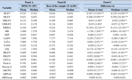
Table 3 presents the descriptive statistics for SPOS (in Panel A) and the rest of the sample (in Panel B); and also compare the SPOS with the rest of the sample in Panel C. Compared with the rest of the sample,
SPOS have a higher book leverage (0.723 vs. 0.616) and market leverage (0.621 vs. 415). These results confirm the findings of Gao and Zhu (2015) and An et al. (2016). The mean book leverage deviation for SPOS is significantly higher than the rest of the sample (0.123 vs. 0.109). Furthermore, SPOS have significantly higher mean market leverage deviation than other firm-years (0.131 vs. 0.116). These results provide primary evidence consistent with Hypothesis I. The mean-scaled CFO for SPOS (0.070 of total assets) is significantly lower than the mean for the
other firm-years (0.160). Furthermore, mean
discretionary expenses scaled by total assets for SPOS are significantly lower than the mean for the rest of sample (0.058 and 0.063, respectively). Nevertheless, the mean-scaled production costs of the SPOS (0.785 of total assets) are significantly higher than the mean for other firms (0.735). Also, as expected, the mean ABCFO and the mean ABProd for SPOS are significantly higher than the mean for other firm-years (0.054 vs. -0.025 for ABCFO, and 0.069 vs. -0.019 for ABProd). However, the mean of ABDisexp is similar in SPOS and other firms (0.002 and -0.003, respectively); and is not significantly different. These results provide preliminary evidence on sales manipulation and overproduction.
Table 2. Descriptive statistics for the main variables
Variable N Mean SD Min. Q1 Median Q3 Max
Table 3. Mean and median for key variables in SOPS and other firm-years
Panel A Panel B Panel C
Variable SPOS (N=287) Rest of the sample (N=4,301) Difference in
Mean Median Mean Median Means (t-stat) Medians (z-stat)
BLEV 0.723 0.763 0.616 0.634 0.107 (13.54)*** 0.129 (14.20)*** MLEV 0.621 0.655 0.415 0.405 0.206 (19.99)*** 0.250 (18.36)*** DBLEV 0.123 0.108 0.109 0.085 0.013 (1.69)* 0.022 (2.09)** DMLEV 0.131 0.129 0.116 0.092 0.015 (1.89)* 0.037 (2.79)***
EBIDA 0.104 0.097 0.224 0.211 -0.120 (-22.32)*** -0.114 (-22.10)*** MB 2.400 1.578 3.538 2.474 -1.138 (-7.84)*** -0.896 (-10.10)*** DEP 0.070 0.057 0.067 0.058 0.004 (2.15)** -0.001 (-0.35) LnMV 7.669 7.596 7.377 7.316 0.292 (7.93)*** 0.280 (7.86)***
LnTA 5.809 5.758 5.728 5.657 0.081 (2.67)*** 0.102 (2.63)*** TANG 0.292 0.218 0.272 0.226 0.020 (2.31)** -0.008 (-0.19)
LIQ 1.122 1.039 1.296 1.182 -0.174 (-6.78)*** -0.143 (-8.23)*** IBLEV 0.689 0.695 0.668 0.684 0.021 (4.84)*** 0.011 (4.49)*** IMLEV 0.494 0.504 0.442 0.461 0.052 (8.86)*** 0.043 (8.41)*** CFO/A 0.070 0.061 0.160 0.142 -0.090 (-10.34)*** -0.081 (-10.38)*** Prod/A 0.785 0.691 0.735 0.641 0.050 (2.06)** 0.049 (2.27)** Disexp/A 0.058 0.049 0.063 0.053 -0.005 (-2.03)** -0.004 (-2.25)**
ABCFO 0.054 0.060 -0.025 -0.008 0.079 (9.17)*** 0.068 (9.12)*** ABProd 0.069 0.055 -0.019 -0.008 0.088 (10.06)*** 0.063 (10.44)*** ABDisexp 0.002 0.005 -0.003 0.004 0.005 (0.23) 0.001(0.02)
*, ** and *** represent significance at the 10% , 5% and 1% level, respectively.
4.2. Model estimation
4.2.1. Manipulation of real activities
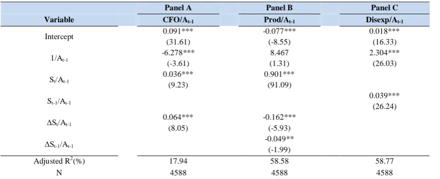
Table 4 reports the estimation results of models (1), (2) and (3), which are used to estimate the abnormal level of CFO, production costs, and discretionary expenses, respectively.
More specifically, Table 4 reports the mean coefficient estimates, associated t-statistics (calculated using the mean standard errors), and the mean adjusted R2s across all industry-years for each of the regression models. The sign of coefficients is consistent with previous studies (e.g., Cupertino et al., 2015; Roychowdhury, 2006). In models (1) and (2), the coefficient of St/At-1 (0.360 and 0.901, respectively) and in model (3) the coefficient of St-1/At-1 (0.039) are significant at the 1% level. The mean adjusted R2s is 18%, 59%, and 59% for models (1), (2), and (3), respectively.
4.2.2. ABCFO, ABProd, and ABDisexp in SPOS Table 5 reports the estimation results of model (4) for ABCFO, ABProd, and ABDisexp as dependent variables.
Panel A (Panel B) represents the estimation results using raw (demeaned) control variables. In Panel A, when the dependent variable is ABCFO, β1 is significantly positive (0.090, t= 1.85), as predicted. Furthermore, β1 is 0.031 (t=2.13) when ABProd is the dependent variable. Also, when ABDisexp is the dependent variable, β1 is significantly positive (0.052, t= 2.90). When demeaned control variables are used (in Panel B), we find more robust evidence consistent with manipulating sales, overproduction and abnormal reduction of discretionary expenses in SPOS.
4.2.3. Target leverage regression and total leverage deviation
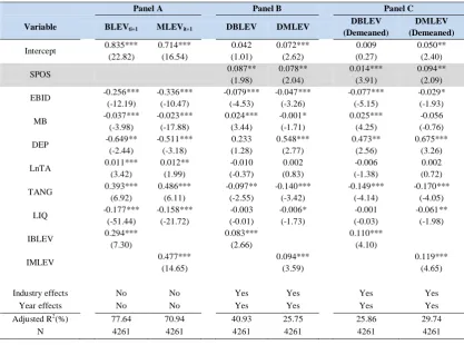
Panel A in Table 6 represents the estimation results of model (5) for book leverage and market leverage as dependent variables.
More specifically, Panel A reports the mean coefficient estimates, associated t-statistics (calculated using the mean standard errors), and the mean adjusted R2s across industry-years for each of the regression models. The signs of target leverage determinants (for both book leverage and market leverage) are generally consistent with the existing literature such as Öztekin and Flannery (2012) and Zhou et al. (2016). The first and second columns of Panel B report the estimation results of model (6) for DBLEV and DMLEV as dependent variables when using raw control variables. Panel C presents the estimation results using demeaned control variables. Furthermore, in Panels B and C, industry and year effects are controlled by adding industry and year dummies to the regression models.
Hypothesis I predicts that SPOS display higher leverage deviation than other firm-years. More specifically, according to Hypothesis I, we expect a positive sign for ϕ in the model (6). Consistent with this, in the first column of panel B, ϕ is 0.087 (t=1.98); and in the second column ϕ is 0.078 (t=2.04). Panel C provides similar results to Panel B. Overall; these
results show that SPOS have a significantly higher total leverage deviation than other firm-years.
4.2.4. Positive and negative leverage deviation in SPOS
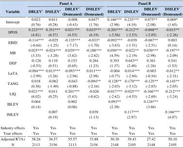
Panels A and B in Table 7 represents the estimation results of model (6) for positive and negative leverage deviation as the dependent variable, respectively. Hypothesis II predicts that SPOS show the higher positive leverage deviation than other firm-years. Specifically, when the dependent variable is the positive deviation from target leverage, we expect a positive sign for ϕ in model (6). Consistent with this, in the first column of Panel A, ϕ is 0.223 (t=4.81) when DBLEV+ is the dependent variable. When DMLEV+ is the dependent variable, ϕ is significantly positive (0.351, t= 6.57), as predicted.
Using the demeaned control variables provides similar results in support of Hypothesis II (the third and the fourth columns in Panel A). Furthermore, Hypothesis III predicts that in model (6), ϕ should be negative with the negative leverage deviation as the dependent variable. We find statistically strong evidence of unusually low DBLEV- (-0.203, t=-3.56) and DMLEV- (-0.212, t= -2.53) for SPOS. Furthermore, using the demeaned control variables shows similar results in support of Hypothesis III (the third and the fourth columns in Panel B).
Table 4. The estimation results of real activities manipulation models
Panel A Panel B Panel C
Variable CFO/At-1 Prod/At-1 Disexp/At-1
Intercept 0.091*** (31.61)
-0.077*** (-8.55)
0.018*** (16.33) 1/At-1 -6.278***
(-3.61)
8.467 (1.31)
2.304*** (26.03) St/At-1 0.036***
(9.23)
0.901*** (91.09)
St-1/At-1 0.039***
(26.24) ΔSt/At-1 0.064***
(8.05)
-0.162*** (-5.93)
ΔSt-1/At-1 -0.049**
(-1.99)
Adjusted R2(%) 17.94 58.58 58.77
N 4588 4588 4588
Table 5. ABCFO, ABProd, and ABDisexp in SPOS
Panel A Panel B
Variable ABCFO ABProd ABDisexp ABCFO
(Demeaned)
ABProd (Demeaned)
ABDisexp (Demeaned)
Intercept 0.146*** (6.30) -0.062*** (-2.57) -0.021* (-1.73) 0.006 (0.63) 0.070*** (3.22) 0.066*** (2.82) SPOS 0.090*
(1.85) 0.031** (2.13) 0.052*** (2.90) 0.067*** (10.40) 0.091*** (30.53) 0.067*** (5.91) LnMV -0.011***
(-3.42) -0.058* (-1.87) 0.033*** (2.93) -0.022*** (-4.25) 0.016*** (2.99) 0.031** (2.20) MB -0.040***
(-4.65) 0.033 (0.45) -0.059*** (-3.20) -0.096*** (-5.88) -0.019 (-1.61) -0.134*** (-6.90) EBIDA -0.665***
(-27.39) 0.783** (42.88) -0.061 (-0.91) -0.079*** (-3.16) -0.015 (-0.73) -0.039 (-0.90)
Industry effects Yes Yes Yes Yes Yes Yes
Year effects Yes Yes Yes Yes Yes Yes
Adjusted R2(%) 50.67 56.61 58.31 54.68 69.43 57.46
N 4588 4588 4588 4588 4588 4588
*, ** and *** represent significance at the 10%, 5% and 1% level, respectively.
Table 6. Target leverage regression and total leverage deviation
Panel A Panel B Panel C
Variable BLEVti+1 MLEVit+1 DBLEV DMLEV
DBLEV (Demeaned)
DMLEV (Demeaned)
Intercept 0.835*** (22.82) 0.714*** (16.54) 0.042 (1.01) 0.072*** (2.62) 0.009 (0.27) 0.050** (2.40)
SPOS 0.087**
(1.98) 0.078** (2.04) 0.014*** (3.91) 0.094** (2.09) EBID -0.256***
(-12.19) -0.336*** (-10.47) -0.079*** (-4.53) -0.047*** (-3.26) -0.077*** (-5.15) -0.029* (-1.93) MB -0.037***
(-3.98) -0.023*** (-17.88) 0.024*** (3.44) -0.001* (-1.71) 0.025*** (4.25) -0.056 (-0.76) DEP -0.649**
(-2.44) -0.511*** (-3.18) 0.233 (1.28) 0.548*** (2.77) 0.473** (2.56) 0.675*** (3.26) LnTA 0.011***
(3.42) 0.012** (1.99) -0.010 (-0.37) 0.002 (0.83) -0.006 (-1.38) 0.002 (0.72) TANG 0.393***
(6.92) 0.486*** (6.11) -0.097** (-2.55) -0.140*** (-3.42) -0.149*** (-4.14) -0.170*** (-4.05) LIQ -0.177***
(-51.44) -0.158*** (-21.72) -0.003 (-0.01) -0.006* (-1.73) -0.001 (-0.03) -0.061** (-1.98) IBLEV 0.294***
(7.30)
0.083*** (2.66)
0.110*** (4.10)
IMLEV 0.477***
(14.65)
0.094*** (3.59)
0.119*** (4.65)
Industry effects No No Yes Yes Yes Yes
Year effects No No Yes Yes Yes Yes
Adjusted R2(%) 77.64 70.94 40.93 25.75 25.86 29.74
*, ** and *** represent significance at the 10%, 5% and 1% level, respectively.
Table 7. Positive and negative leverage deviation in SPOS
Panel A Panel B
Variable DBLEV+ DMLEV+ DBLEV +
(Demeaned)
DMLEV+
(Demeaned) DBLEV
- DMLEV- DBLEV
-(Demeaned)
DMLEV
-(Demeaned)
Intercept 0.023 (0.76) 0.011 (0.28) -0.008 (-0.43) 0.047* (1.76) 0.166*** (2.98) 0.235*** (4.10) 0.075** (2.08) 0.069* (1.65) SPOS 0.223***
(4.81) 0.351*** (6.57) 0.021*** (4.53) 0.033*** (6.19) -0.203*** (-3.56) -0.212** (-2.53) -0.068** (-2.05) -0.015** (-2.26) EBID -0.114***
(-6.64) -0.025 (-1.25) -0.135*** (-7.17) -0.033* (-1.70) -0.092*** (-3.63) -0.039 (-1.51) -0.067** (-2.51) 0.003 (0.14) MB 0.025***
(3.33) -0.024*** (-3.28) 0.029*** (3.62) -0.188*** (-2.62) 0.050*** (4.59) -0.022** (-2.19) 0.030*** (2.98) -0.197** (-2.09) DEP -0.126
(-0.53) 0.110 (0.51) 0.153 (0.65) 0.264 (1.23) 0.393 (1.37) 0.643** (2.40) 0.361 (1.26) 0.541 (1.53) LnTA -0.094***
(-2.99) 0.013*** (3.26) -0.093*** (-2.96) 0.011*** (2.98) -0.004 (-0.77) -0.014*** (-2.94) -0.003 (-0.54) -0.012** (-2.31) TANG 0.018
(0.36) -0.062 (-1.40) -0.043 (-0.88) -0.094** (-2.16) -0.128** (-2.03) -0.170*** (-3.12) -0.125** (-2.03) -0.145** (-2.05) LIQ 0.021***
(6.02) 0.011 (0.25) 0.201*** (5.43) -0.026 (-0.62) -0.017*** (-2.62) -0.025*** (-4.53) -0.166*** (-2.69) -0.212*** (-3.24) IBLEV 0.004
(0.14) 0.002 (0.06) 0.093** (2.38) 0.126*** (3.66) IMLEV 0.007
(0.19) 0.039 (1.13) 0.117*** (2.97) 0.166*** (4.07)
Industry effects Yes Yes Yes Yes Yes Yes Yes Yes Year effects Yes Yes Yes Yes Yes Yes Yes Yes Adjusted R2(%) 38.26 36.57 55.57 33.88 30.30 39.43 27.42 50.10
N 2113 2156 2113 2156 2148 2105 2148 2105 *, ** and *** represent significance at the 10%, 5% and 1% level, respectively.
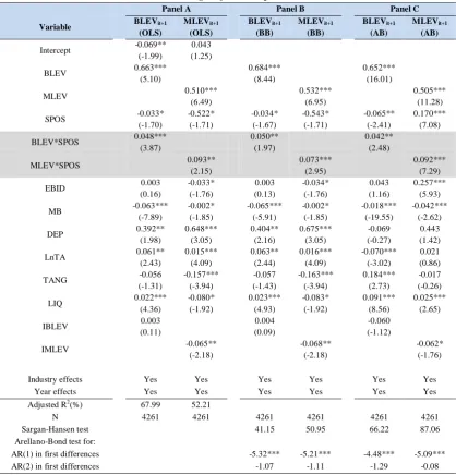
4.2.5. Leverage adjustment speed in SPOS
Table 8 shows the results for Hypothesis IV, which focuses on comparing the leverage adjustment speed in SPOS with the rest of the sample.
Panel A represents the estimation results of model (9) using pooled OLS. Furthermore, Panels B and C represent the estimation results using system-GMM (BB) and difference-GMM (AB), respectively. Hypothesis IV predicts that SPOS display lower leverage adjustment speed than other firm-years. More specifically, we expect a positive sign for η2 in model (9). Consistent with this, in the first column of panel A, η2 is 0.048 (t=3.87); and in the second column, η2 is 0.093 (t=2.15). In panel B, when the dependent variable is BLEVit+1, η2 is significantly positive
Table 8. Leverage adjustment speed in SPOS
Panel A Panel B Panel C
Variable BLEVit+1
(OLS) MLEVit+1 (OLS) BLEVit+1 (BB) MLEVit+1 (BB) BLEVit+1 (AB) MLEVit+1 (AB)
Intercept -0.069** (-1.99)
0.043 (1.25) BLEV 0.663***
(5.10)
0.684*** (8.44)
0.652*** (16.01)
MLEV 0.510***
(6.49)
0.532*** (6.95)
0.505*** (11.28) SPOS -0.033*
(-1.70) -0.522* (-1.71) -0.034* (-1.67) -0.543* (-1.71) -0.065** (-2.41) 0.170*** (7.08) BLEV*SPOS 0.048***
(3.87)
0.050** (1.97)
0.042** (2.48)
MLEV*SPOS 0.093**
(2.15)
0.073*** (2.95)
0.092*** (7.29)
EBID 0.003
(0.16) -0.033* (-1.76) 0.003 (0.13) -0.034* (-1.76) 0.043 (1.16) 0.257*** (5.93) MB -0.063***
(-7.89) -0.002* (-1.85) -0.065*** (-5.91) -0.002* (-1.85) -0.018*** (-19.55) -0.042*** (-2.62) DEP 0.392**
(1.98) 0.648*** (3.05) 0.404** (2.16) 0.675*** (3.05) -0.069 (-0.27) 0.443 (1.42) LnTA 0.061**
(2.43) 0.015*** (4.09) 0.063** (2.44) 0.016*** (4.09) -0.070*** (-3.02) 0.021 (0.86) TANG -0.056
(-1.31) -0.157*** (-3.94) -0.057 (-1.43) -0.163*** (-3.94) 0.184*** (2.73) -0.017 (-0.26) LIQ 0.022***
(4.36) -0.080* (-1.92) 0.023*** (4.93) -0.083* (-1.92) 0.091*** (8.56) 0.025*** (2.65) IBLEV 0.003
(0.11)
0.004 (0.09)
-0.060 (-1.12)
IMLEV -0.065**
(-2.18)
-0.068** (-2.18)
-0.062* (-1.76)
Industry effects Yes Yes Yes Yes Yes Yes
Year effects Yes Yes Yes Yes Yes Yes
Adjusted R2(%) 67.99 52.21
N 4261 4261 4261 4261 4261 4261
Sargan-Hansen test 41.15 50.95 66.22 87.06 Arellano-Bond test for:
AR(1) in first differences -5.32*** -5.21*** -4.48*** -5.09*** AR(2) in first differences -1.07 -1.11 -1.29 -0.08
*, ** and *** represent significance at the 10%, 5% and 1% level, respectively.
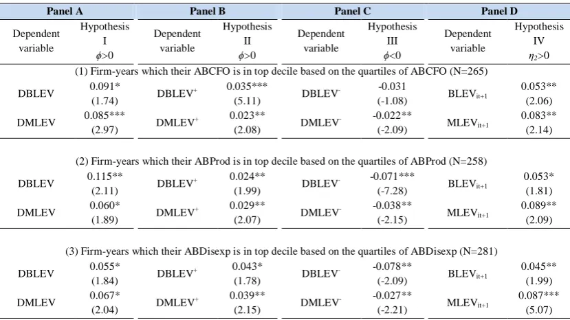
4.3. Additional robustness tests
Using alternative measures to define SPOS, we examine the robustness of the key results. As mentioned earlier, manipulating sales, overproduction, and reduction in discretionary expenses lead to abnormally high values for ABCFO, ABProd, and
ABDisexp, respectively. Accordingly, we use the following four measures to define SPOS: (1) if the firm-years belong to the top decile sorted by ABCFO,
equals to 1 and zero otherwise, (2) if the
firm-years belong to the top decile sorted by ABProd,
firm-years belong to the top decile sorted by ABDisexp,
equals to 1 and zero otherwise, and (4) if the
firm-years belong to the top decile sorted by ABCFO,
ABProd, and ABDisexp, simultaneously,
equals to 1 and zero otherwise. We also define SPOS as those observations which their reported EBID is between zero and 0.01 of total stock market value, as the fifth measure. Using each of these five measures, we re-estimate the corresponding regression models to test the research hypotheses. The corresponding regressions for testing Hypothesis I to Hypothesis III
are estimated using raw control variables
8
.The results of the robustness checks are presented in Table 9. Panel A in Table 9 presents the results of robustness test for Hypothesis I, which predicts that SPOS exhibit higher leverage deviation than other firm-years. From Panel A, we can see that as predicted, ϕ is significantly positive (except for the fourth measure of SPOS when using DBLEV as the
dependent variable). Panels B and C in Table 9 present the robustness test results for Hypothesis II and Hypothesis III, respectively. Hypothesis II (Hypothesis III) predicts that SPOS exhibit higher positive (lower negative) leverage deviation compared with other firm-years. Consistent with this, in panel B, ϕ is significantly positive and in panel C, ϕ is significantly negative (except for the first measure of SPOS when using DBLEV as the dependent variable). Finally, Panel D displays the results of robustness test for Hypothesis IV, which predicts that SPOS exhibit lower leverage adjustment speed compared with other firm-years. Consistent with this, the results are robust to alternative measures of SPOS. Generally, the main results of all research hypotheses remain valid. However, it should be noted that when using the fourth (first) measures of SPOS, we cannot find strong evidence in support of Hypothesis I (Hypothesis III).
Table 9. Additional robustness tests
Panel A Panel B Panel C Panel D
Dependent variable
Hypothesis I
ϕ>0
Dependent variable
Hypothesis II
ϕ>0
Dependent variable
Hypothesis III
ϕ<0
Dependent variable
Hypothesis IV
η2>0
(1) Firm-years which their ABCFO is in top decile based on the quartiles of ABCFO (N=265) DBLEV 0.091*
(1.74) DBLEV
+ 0.035***
(5.11) DBLEV
- -0.031
(-1.08) BLEVit+1
0.053** (2.06) DMLEV 0.085***
(2.97) DMLEV
+ 0.023**
(2.08) DMLEV
- -0.022**
(-2.09) MLEVit+1
0.083** (2.14)
(2) Firm-years which their ABProd is in top decile based on the quartiles of ABProd (N=258)
DBLEV 0.115**
(2.11) DBLEV
+ 0.024**
(1.99) DBLEV
- -0.071***
(-7.28) BLEVit+1
0.053* (1.81) DMLEV 0.060*
(1.89) DMLEV
+ 0.029**
(2.07) DMLEV
- -0.038**
(-2.15) MLEVit+1
0.089** (2.09)
(3) Firm-years which their ABDisexp is in top decile based on the quartiles of ABDisexp (N=281) DBLEV 0.055*
(1.84) DBLEV
+ 0.043*
(1.78) DBLEV
- -0.078**
(-2.09) BLEVit+1
0.045** (1.99) DMLEV 0.067*
(2.04) DMLEV
+ 0.039**
(2.15) DMLEV
- -0.027**
(-2.21) MLEVit+1
0.087*** (5.07)
(4) Firm-years which their ABCFO, ABProd, and ABDisexp are in top decile based on the quartiles of them, simultaneously (N=179)
DBLEV 0.053
(1.27) DBLEV
+ 0.016**
(2.14) DBLEV
- -0.055*
(-1.91) BLEVit+1
0.055** (2.14) DMLEV 0.044*
(1.77) DMLEV
+ 0.022*
(1.83) DMLEV
- -0.013*
(-1.79) MLEVit+1
0.103* (1.70)
DBLEV 0.085**
(2.13) DBLEV
+ 0.027***
(5.71) DBLEV
- -0.073***
(-3.35) BLEVit+1
0.058** (2.06) DMLEV 0.094***
(3.09) DMLEV
+ 0.042***
(6.19) DMLEV
- -0.024**
(-2.19) MLEVit+1
0.090** (2.16) *, ** and *** represent significance at the 10%, 5% and 1% level, respectively.
5. Discussion and Conclusions
Earnings management literature suggests that compared to other firms, SPOS are more likely to manipulate their real activities. This paper compares the deviation from target leverage and leverage adjustment speed in SPOS with other firms. Our sample consists of Iranian firms listed in Tehran Stock Exchange, and we collect data from CODAL, RDIS and Rahavard Nowin database. We use 4588 firm-year observations from 2003 to 2016.
Consistent with the previous literature, we first provide evidence showing that SPOS engage in real activities manipulation and have a higher leverage ratio. Next, we express target leverage as a linear function of firm and industry characteristics and calculate total leverage deviation as actual leverage minus the fitted values from the regression of leverage ratio on determinants of capital structure. Then, we calculate positive and negative leverage deviation. After that, we compare total, positive, and negative leverage deviation in SPOS with the rest of the sample. Previous studies use earnings management as a measure of information quality (Leuz, Nanda, & Wysocki, 2003) or information asymmetry (e.g., An et al., 2016; Bhattacharya et al., 2003; Lang et al., 2012) and indicate that earnings management positively affects leverage ratios (An et al., 2016). Our findings on SPOS confirm the previous results. We find evidence suggesting that book leverage and market leverage in SPOS are higher than that of other firm-years. Considering raw and demeaned control variables, we show that SPOS have a higher total leverage deviation than other firm-years. We also find that in SPOS, the positive (negative) leverage deviation is higher (lower) than that of other firms. Finally, we test whether SPOS have a lower leverage adjustment speed compared with the other firms. The results indicate that compared with other firms, SPOS have a slower adjustment speed toward the target leverage. In general, results indicate that real activities manipulation in SPOS can lead to a sub-optimal leverage ratio and lower leverage adjustment speed.
References
1) Abad, D., Cutillas-Gomariz, M. F.,
Sánchez-Ballesta, J. P., & Yagüe, J. (2018). Real earnings management and information asymmetry in the equity market. European Accounting Review,
27(2), 209-235.
doi:10.1080/09638180.2016.1261720
2) Agarwal, P., & O'Hara, M. (2007). Information
risk and capital structure. Cornell University. Retrieved from https://ssrn.com/abstract=939663
3) An, Z., Li, D., & Yu, J. (2016). Earnings
management, capital structure, and the role of institutional environments. Journal of Banking and
Finance, 68, 131-152.
doi:https://doi.org/10.1016/j.jbankfin.2016.02.007
4) Arellano, M., & Bond, S. (1991). Some tests of
specification for panel data: Monte Carlo evidence and an application to employment equations. The review of economic studies, 58(2), 277-297.
5) Bharath, S. T., Pasquariello, P., & Wu, G. (2008).
Does asymmetric information drive capital structure decisions? The Review of Financial Studies, 22(8), 3211-3243.
6) Bhattacharya, U., Daouk, H., & Welker, M.
(2003). The world price of earnings opacity. The
Accounting Review, 78(3), 641-678.
doi:10.2308/accr.2003.78.3.641
7) Blundell, R., & Bond, S. (1998). Initial conditions
and moment restrictions in dynamic panel data models. Journal of Econometrics, 87(1), 115-143. doi:https://doi.org/10.1016/S0304-4076(98)00009-8
8) Brown, S., Hillegeist, S. A., & Lo, K. (2009). The
effect of earnings surprises on information asymmetry. Journal of Accounting and Economics,
47(3), 208-225.
doi:https://doi.org/10.1016/j.jacceco.2008.12.002
9) Burgstahler, D., & Dichev, I. (1997). Earnings
10)Byoun, S. (2008). How and when do firms adjust their capital structures toward targets? The Journal
of Finance, 63(6), 3069-3096.
doi:doi:10.1111/j.1540-6261.2008.01421.x
11)Chen, W., Hribar, P., & Melessa, S. (2017).
Incorrect inferences when using residuals as dependent variables. Journal of Accounting
Research, Advance online publication.
doi:10.1111/1475-679X.12195
12)Cohen, D. A., Dey, A., & Lys, T. Z. (2008). Real and accrual-based earnings management in the pre-and post-Sarbanes-Oxley periods. The Accounting Review, 83(3), 757-787.
13)Cormier, D., Houle, S., & Ledoux, M.-J. (2013). The incidence of earnings management on
information asymmetry in an uncertain
environment: Some Canadian evidence. Journal of International Accounting, Auditing and Taxation,
22(1), 26-38.
doi:https://doi.org/10.1016/j.intaccaudtax.2013.02. 002
14)Cupertino, C. M., Martinez, A. L., & da Costa, N.
C. A. (2015). Earnings manipulations by real activities management and investors’ perceptions. Research in International Business and Finance,
34, 309-323.
doi:https://doi.org/10.1016/j.ribaf.2015.02.015
15)Dang, V. A., Kim, M., & Shin, Y. (2012).
Asymmetric capital structure adjustments: New evidence from dynamic panel threshold models. Journal of Empirical Finance, 19(4), 465-482. doi:https://doi.org/10.1016/j.jempfin.2012.04.004
16)Dechow, P. M., & Schrand, C. M. (2004).
Earnings Quality. Charlottesville, VA: Research Foundation of CFA Institute.
17)Flannery, M. J., & Hankins, K. W. (2013).
Estimating dynamic panel models in corporate finance. Journal of Corporate Finance, 19, 1-19. 18)Flannery, M. J., & Rangan, K. P. (2006). Partial
adjustment toward target capital structures. Journal of financial economics, 79(3), 469-506.
19)Gao, W., & Zhu, F. (2015). Information
asymmetry and capital structure around the world. Pacific-Basin Finance Journal, 32, 131-159. doi:https://doi.org/10.1016/j.pacfin.2015.01.005
20)He, W. P., Lepone, A., & Leung, H. (2013).
Information asymmetry and the cost of equity capital. International Review of Economics &
Finance, 27, 611-620.
doi:https://doi.org/10.1016/j.iref.2013.03.001
21)Healy, P. M., & Wahlen, J. M. (1999). A review of
the earnings management literature and its implications for standard setting. Accounting horizons, 13(4), 365-383.
22)Lambert, R., Leuz, C., & Verrecchia, R. E. (2007).
Accounting information, disclosure, and the cost of capital. Journal of Accounting Research, 45(2), 385-420.
23)Lang, M., Lins, K. V., & Maffett, M. (2012).
Transparency, liquidity, and valuation:
International evidence on when transparency matters most. Journal of Accounting Research, 50(3), 729-774.
24)Leuz, C., Nanda, D., & Wysocki, P. D. (2003).
Earnings management and investor protection: an international comparison. Journal of Financial
Economics, 69(3), 505-527.
doi:https://doi.org/10.1016/S0304-405X(03)00121-1
25)Lombardo, D., & Pagano, M. (2002). Law and
equity markets: A simple model. Corporate governance regimes: Convergence and diversity, 343-362.
26)Marchica, M. T., & Mura, R. (2010). Financial
flexibility, investment ability, and firm value: evidence from firms with spare debt capacity. Financial management, 39(4), 1339-1365.
27)Mashayekhi, B., & Mashayekh, S. (2008).
Development of accounting in Iran. The International Journal of Accounting, 43(1), 66-86. doi:https://doi.org/10.1016/j.intacc.2008.01.004 28)Mehrani, S., Moradi, M., & Eskandar, H. (2017).
Institutional ownership type and earnings quality: Evidence from Iran. Emerging Markets Finance
and Trade, 53(1), 54-73.
doi:10.1080/1540496X.2016.1145114
29)Miglo, A. (2016). Asymmetric Information and
Capital Structure. In Capital Structure in the Modern World (pp. 45-67). Cham: Springer International Publishing.
30)Modigliani, F., & Miller, M. H. (1958). The cost of capital, corporation finance and the theory of investment. The American Economic Review, 48(3), 261-297.
31)Öztekin, Ö., & Flannery, M. J. (2012). Institutional
88-112.
doi:https://doi.org/10.1016/j.jfineco.2011.08.014
32)Petacchi, R. (2015). Information asymmetry and
capital structure: Evidence from regulation FD. Journal of Accounting and Economics, 59(2), 143-162.
doi:https://doi.org/10.1016/j.jacceco.2015.01.002
33)Richardson, V. J. (2000). Information asymmetry
and earnings management: Some evidence. Review of Quantitative Finance and Accounting, 15(4), 325-347. doi:10.1023/a:1012098407706
34)Roychowdhury, S. (2006). Earnings management
through real activities manipulation. Journal of Accounting and Economics, 42(3), 335-370. doi:https://doi.org/10.1016/j.jacceco.2006.01.002 35)Supra, B., Narender, V., Jadiyappa, N., & Girish,
G. (2016). Speed of adjustment of capital structure in emerging markets. Theoretical Economics Letters, 6(03), 534-538.
36)Synn, C. J., & Williams, C. D. (2015). Financial reporting quality and optimal capital structure. Paper presented at the The 8th CAPANA annual
research conference. www. capana.
net/www/conference2015/Syn nWilliams. pdf.
37)Uysal, V. B. (2011). Deviation from the target
capital structure and acquisition choices. Journal of
Financial Economics, 102(3), 602-620.
doi:https://doi.org/10.1016/j.jfineco.2010.11.007 38)Zhou, Q., Tan, K. J. K., Faff, R., & Zhu, Y.
(2016). Deviation from target capital structure, cost of equity and speed of adjustment. Journal of
Corporate Finance, 39, 99-120.
doi:https://doi.org/10.1016/j.jcorpfin.2016.06.002
Notes
1
www.audit.org.ir 2
www.codal.ir 3
www.rdis.ir/CompaniesReports.asp 4 www.mabnadp.com/rahavardnovin3 5
http://new.tse.ir/en/
6 R&D expenditure is zero for the vast majority of Iranian firms.
7 Because of high inflation rate in Iran, we also use logarithm of sales revenues and logarithm of total stock market values as proxies for firm size. Un-tabulated key results remain robust to these proxies.