Estimating a Bounded Normal Mean
Under the LINEX Loss Function
A. Karimnezhad
*Department of Statistics, Faculty of Mathematics, Statistics and Computer Science, University of Tehran, Tehran, Islamic Republic of Iran
Received: 18 January 2013 / Revised: 13 May 2013 / Accepted: 1 July 2013
Abstract
Let
X
be a random variable from a normal distribution with unknown mean
θ
and known variance
σ
2. In many practical situations,
θ
is known in advance to lie
in an interval, say [
−m
,
m
], for some
m
> 0. As the usual estimator of
θ
, i.e.,
X
under the LINEX loss function is inadmissible, finding some competitors for
X
becomes worthwhile. The only study in the literature considered the problem of
minimax estimation of
θ
In this paper, by constructing a dominating class of
estimators, we show that the maximum likelihood estimator is inadmissible. Then,
as a competitor, the Bayes estimator associated with a uniform prior on the
interval [
−m
,
m
] is proposed. Finally, considering risk performance as a
comparison criterion, the estimators are compared and depending on the values
taken by
θ
in the interval [
−m
,
m
], the appropriate estimator is suggested.
Keywords: Admissibility; Bayes estimator; LINEX loss function; Maximum likelihood estimator; Normal distribution
* Corresponding author, Tel.: +98(21)61112624, Fax: +98(21)66412178, E-mail: [email protected] Introduction
In the statistical literature it is often assumed that the parameter space is unbounded which seems to be never fulfilled in practice. In various physical, industrial and biological experiments, the experimenter has often some prior knowledge about the parameter(s) of the underlying population. The average per capita income of a developing country is likely to lie between those of an underdeveloped and a developed country. The average fuel efficiency of a new model of passenger car will lie between those of an old model and a formula one racing car. Examples of similar nature where mean of a real phenomena lies in a bounded interval abound in practice (e.g., physical attributes such as height or
weight of people, average life of animals), [14]. Therefore there is practical interest to include such additional information into statistical procedures.
Surprisingly, while the assumption of boundedness can be useful in practice, it introduces some challenging problems in theory. Such problems first arose with the practical problem in 1950 in which two probabilities 1
and 2 known to satisfy the restriction 1 2, needed
to be estimated. Maximum likelihood estimation was used for this purpose. Later Maximum Likelihood Estimators (MLEs) were shown to be inadmissible under Squared Error Loss (SEL) function
2
( , ) ( ) ,
that is, it was shown that there exist estimators which are better than the MLE in the sense that their expected loss, i.e., R( , ) E L[ ( , )] , as a function of the parameter to be estimated, is nowhere larger and somewhere smaller than that of the MLE. This then led to the search for dominators for these inadmissible estimators as well as for admissible estimators with “good properties”. One such property is that of minimaxity where an estimator is minimax when there does not exist an estimator with a smaller maximum expected loss. Examples of problems addressed in the restricted parameter spaces, can be found in [1], [17], [26] and the recent treatise by ven Eeden [27] for detailed discussion.
Let X ~N( , 2) denote a random variable having
normal distribution with the probability density function 2
2
1 ( )
2 2
2
1
( | , ) , ,
2
x
f x e x
where, it is supposed that the variance 2 is known and
the unknown mean , lies in an interval of the form [m m, ], for some known m > 0. The first study in estimating the bounded normal mean under the SEL function dates back to 1981. Casella and Strawderman [4] showed that, when 0 m m01.05, there exists a
unique admissible and minimax estimator of ,
associated with a symmetric two-point prior on
m m,
and proved that it dominates the MLE of , when 0 m 1. They also gave a class of admissible and minimax estimators for the case when 1.4m1.6. These estimators are minimax w.r.t. a symmetric three-point prior on
m,0,m
. Bickel [2] presented an estimator which is asymptotically minimax as m , and showed that the weak limit of the least favourable prior (rescaled to [ 1,1] ) has the density2 ,
2 cos
| | 1 and the minimax risk is
2 2 2
1 m o m( ). After these initial works, several
authors considered the estimation problem in restricted parameter spaces under the SEL function. Moors [18, 19] assumed a bounded estimation problem is invariant w.r.t. a finite group of transformations and constructed dominators of a boundary estimator. He then applied his results into the estimation problem of a bounded normal mean. Gatsonis et al. [10] considered the Bayes estimator w.r.t. the uniform prior on the interval [m m, ], as a competitor for the sample mean X, and showed that it dominates X . They further numerically compared risk performance of their Bayes estimator, the
MLE, the minimax estimator, and the Bayes estimator w.r.t. the Bickel’s prior, and finally recommended the use of their proposed estimator. In addition to [18, 19], the estimation in restricted parameter spaces under the SEL function, in a very general setting, was considered in [5, 6, 7]. DasGupta [7] in estimating a vector h( )
when is restricted to a small bounded convex subset
of k derived sufficient conditions under which the
Bayes estimator w.r.t. a least favourable prior on the boundary of is minimax. He then applied his results in some distributions including the normal distribution and showed that the Bayes estimator w.r.t. the two-point prior considered in [4] is minimax when m 0.643. Conditions for either inadmissibility or methods of constructing dominators within a given class of estimators were presented in [5, 6]. Kumar and Tripathi [14], on the basis of MLE, proposed another estimator and compared the risk performance of it with the above-mentioned estimators. Dou and van Eeden [8], showed the inadmissibility conditions in [5, 6] are satisfied for the bounded normal mean problem and hence, by giving an explicit form of a dominating estimator, derived inadmissibility of MLE of the mean . Lately, the general theory of estimating parameters of a symmetric distribution which is subject to an interval constraint, under the SEL function developed in [16]. See also [15] for a similar development.
It is worth mentioning that the problem of estimating a normal mean in the case where is bounded below, i.e., a, for some constant ,a also received considerable attention in the literature. Estimation of a positive normal mean was first considered in Katz [13]. Katz proposed the generalized Bayes estimator of
w.r.t. the uniform prior on [0, ) and proved its admissibility and minimaxity under the SEL function. He also proved that the restricted MLE, is minimax. The results of Katz were independently proved in [22] and generalized in [9] to a general location parameter family under certain conditions. Thereafter, the problem of estimating a positive normal mean has developed in the literature,seeforexamples[25,26]andreferencestherein.
Some authors have considered an estimation problem under an asymmetric LINEX (LINear EXponential) loss function
( )
, ( , ) { ( ) 1},
a a s
L s e a (1)
where a0 and s 0 are fixed real numbers. This loss function which was first introduced by Varian [28], rises exponentially on one side and approximately linearly on the other side, and is useful when overestimation is perceived as more serious than under-estimation or vice-versa. For more information on point estimation under LINEX loss function, see [20, 29].
In the normal mean
estimation problem with no restriction on
, Zellner [29] showed that the usual estimator X under the LINEX loss function is inadmissible and dominated by2
*( ) .
2 a
X X
(2)
Hence, X is neither admissible nor minimax. Also, Rojo [21] and Sadooghi-Alvandi and Nematollahi [23] proved that in the class of estimators of the form
,
cX d * is the only miniamx and admissible
estimator of
.In the bounded normal case under the LINEX loss function (1), the only study dates back to 1995. Bischoff et al. [3] considered minimax estimation of
and showed that the Bayes estimator w.r.t. the two-point prior( ) 1 ( )
m m m m
i.e.,
, ( ) 1ln ( )
( )
a m
g X X
a g X a
where g x( )emx (1 )emx, is minimax when
0,
a
1 and m(0,m0], 0
1
min 3 1 ,
2
m a
1 ln 3 2a
In this paper, we consider the LINEX loss function (1) and with no loss of generality, we take s1, i.e.,
( , ) a 1, 0.
a
L e a a (3)
We then propose some estimators of the bounded normal mean
and compare risk performance of the proposed ones with the minimax estimator derived in [3]. To this end, first, we obtain conditions under whichthe MLE of , i.e.,
( ) | | .
MLE
m X m
X X X m
m X m
is inadmissible and hence, we derive a class of dominating estimators. We then propose the Bayes estimator of the mean
w.r.t. uniform prior as a competitor for MLE. Finally, we wish to compare risk performance of the derived estimators. Notice that the concept of admissibility, Bayesianity, invariance and minimaxity highly depends on the choice of loss function. It is worth noting that there exist some other works related to restricted parameter estimation problem, considering other losses. For a brief history and some related references, see the recent work done by Karimnezhad [12] which considered the bounded normal mean estimation problem relative to the SEL function.Inadmissibility of MLE
In this section, we construct a dominating class of estimators of MLE based on the work done by Charras
[5] and Charras and van Eeden [6] (readers may refer to [8] as a convenience version of [5, 6]).
Let Ch be a shrinkage estimator of the following
form
( ) | | ,
Ch
m X m
X X X m
m X m
(4)
where (0, ].m Due to the mentioned aim, we first provide some required materials below.
Lemma 1. Let
2
1 2
( ) ( )
( ) ( ), 0,
ax
a
u x e ax x
e x a a x a
(5)
2
1 2
( ) ( )
( ) ( ), 0,
ax
a
v x e ax x
e x a a x a
(6)
where (.) and (.) denote the distribution and density function of a standard normal random variable. Then
( ),
the following properties:
(a) u x( ) and v x( ) are decreasing for x 0 and increasing for x 0.
(b) u x'( )a
1eax
( x) and has the same signas .x
(c) u x''( )a e2 ax ( x) for x 0.
(d) v x'( )a
1eax
( )x and has the same signas .x
(e) v x''( )a e2 ax( )x for x 0.
Proof. The proof is straightforward and omitted.
Lemma 2. Let h x( , ) u'(x)v'(x) where ( )
u x and v x( ) are given by (5) and (6). Further suppose a is positive, then
(a) For fixed (0, )m and for (m, ],m
( , )
h m is a decreasing function of
.(b) For x[0, ],m let
' '
( )x h m x m( , ) u (2m x) v x( ).
(7)
Then (0) 0 and ( ) 0.m Furthermore, if a0 satisfy one of the following conditions:
0
a (8)
or
1 2
0 a 1 and max w a w a( ), ( ) 0 (9) where
2
1( ) 1
am
w a e a (10)
and
2 2
2
( ) ( 2 )
( ) ( ), 2
am
am am
w a ae m
a
m e e m
(11)
then '( ) 0,x for x(0, ).m Hence, there exists a
unique root '(0, )m of the equation ( ) 0x such
that under conditions (8) or (9), for x [0, ),' ( ) 0,x
and for x ( , ],' m ( ) 0.x
Proof.
(a) Differentiating h m( , ) w.r.t. , we have
''
''
( , ) ( )
( ).
h m u m
v m (12)
Now using Lemma 1(c) and (e), the remainder is easily obtained.
(b) Differentiating ( )x w.r.t. ,x we have
'( )x u''(2m x) v x''( ).
On the other side, for x[0, ]m
(13)
Now let
(2 ) 2
( ) a m x ax ax.
w x ae a e ae
We discuss the sign of w x( ). Due to condition (8),
2
a a and hence w x( ) is positive. Moreover under condition (9), it can be easily seen that w x( ) is an increasing function. So using equation (10), for
[0, ],
x m 2 2
1
( ) (0) am ( ).
w x w ae a a aw a Further,
using the following inequalities
2 (2 ) 2 2
(2 ) 2
2 2
( 2 ) ( 2 ),
(2 ) 1 ( ) 1 ,
( ) (0),
( ) 1 0,
a m x am
a m x am
ax am
ax
a e x m a e m
a m x e a m e
a e x a e
a x e
And equations (11) and (13), we conclude that
'' ''
2
(2 ) ( ) ( ).
u m x v x w a Hence, if 0 a 1 and
1 2
max w a w a( ), ( ) 0,u''(2m x )v x''( ) will be
positive and the proof is completed.
The main result of this section is as follows.
Theorem 1. Let X ~N( ,1) when | | m,m0. Then under conditions (8) and (9),
: 0 '
Ch
is a class of dominating estimators of MLE w.r.t. the
LINEX loss function (3), where ' is the unique root of
equation (10).
'' ''2 (2 )
(2 ) 2 (2 ) 2 (2 ) 2
(2 ) 2
(2 ) ( )
( 2 )
(2 ) 1
( ) ( ) 1
(2 ) 1
( ) ( ) 1
(2 ) 1
(2 ) 1
(2 )
a m x
a m x
ax ax
a m x
ax ax
a m x
ax ax
a m x ax ax
u m x v x
a e x m
a m x e
a e x a x e
a m x e
a e x a x e
a m x e
m x a e a e
m x ae a e ae
Proof. Due to equations (5) and (6), it can be easily verify that the risk function of MLE and Ch have the
following form
(14)
and
(15)
Let
(MLE, Ch; , ) R( , MLE) R( , Ch).
Now, we discuss the sign of (MLE, Ch; , ) in two cases. (i) when [ m ,m), using Lemma 1(a) the desired result follows. (ii) when (m, ],m differentiating (MLE, Ch; , ) w.r.t. , according to Lemma 1(a), we have
'
' '
( ) 0, 0
( , ; , ) ( , )
( ) 0, .
MLE Ch h m m
Consequently, for [0, ]' and (m, ],m
(MLE, Ch; , ) (MLE, Ch; ,0) 0
And this completes the proof.
The next lemma which is similar to the work done by Moors [18, 19] and Bischoff et al. [3], provides a useful extension of the main result.
Lemma 3. Suppose an estimation problem is invariant w.r.t. the finite group of transformations G
e g, , where for x
,e x( )x is an identity transformation and g x( ) x. Further suppose for,
x
i( x) i( ),x i 1,2. Then, in the family of normal distributions
N( ,1),
and under the LINEX function (3), for given a0 and [ ,m m1 2],1
dominates 2 if and only if for a0 and
2 1 [ m , m],
.. dominate 2.
Proof. The following relation is held assuming the mentioned assumptions
, ( )
, ( ) ,
1, 2a i a i
EL X EL X i and because of that,
1 2
1 2
, ( ) , ( )
, ( ) , ( ) .
a a
a a
E L X E L X
E L X E L X
This gives the desired result.
Now, using Theorem 1 and Lemma 3, the next theorem is immediately derived.
Theorem 2. Let X ~N( ,1) when | | m m, 0. Then under conditions
1 a
or
1 2
1 a 0 and max w ( ),a w ( )a 0
where w a1( ) and w a2( ) are given in equations (10)
and (11) respectively, for 0 m and [ m m, ],
MLE is inadmissible and
:0 '
Ch is a class of dominating estimators of ,
MLE
where Ch is given in (4) and ' is the unique
root satisfying Theorem 1.
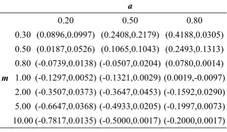
In Table 1, values of
w a w a1( ), 2( )
(given byequations (10) and (11)) for different values of m and a have been tabulated. As it can be seen, when a is positive, at least on of w a1( ) and w a2( ) is positive and
the condition max
w a w a1( ), 2( )
0 is not a limitingone. In the same way, it can be inferred that when a is negative, the condition max
w1( ),a w2( )a
0 is notan encumbrance condition.
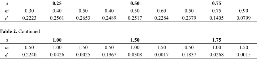
In Table 2, values of the unique root of equation (7) for various values of a and m have been calculated. Notice that under conditions mentioned in Theorem 1, for (0, ]' and [ m , ],m
Ch
dominates MLE
but because of the mathematical difficult computations, it is not easy to prove this property explicitly. This subject in Theorem 2 for (0, ]' and [m, ]m
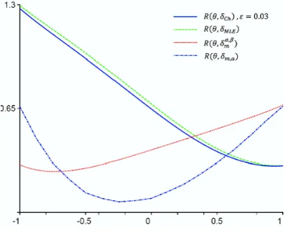
holds but because of the same reason, we cannot prove that. This desired property is obviously seen from Fig. 1
Table 1.Valuesof(w1(a),w2(a))fordifferentvaluesofaandm
a
0.20 0.50 0.80
0.30 (0.0896,0.0997) (0.2408,0.2179) (0.4188,0.0305) 0.50 (0.0187,0.0526) (0.1065,0.1043) (0.2493,0.1313) 0.80 (-0.0739,0.0138) (-0.0507,0.0204) (0.0780,0.0014)
m 1.00 (-0.1297,0.0052) (-0.1321,0.0029) (0.0019,-0.0097) 2.00 (-0.3507,0.0373) (-0.3647,0.0453) (-0.1592,0.0290) 5.00 (-0.6647,0.0368) (-0.4933,0.0205) (-0.1997,0.0073) 10.00 (-0.7817,0.0135) (-0.5000,0.0017) (-0.2000,0.0017)
( , MLE) ( ) ( ) 1
R um vm
( , Ch) ( ) ( ) 1.
to Fig. 6. Moreover when tends to ', the difference
between risk functions of Ch and MLE becomes
significant. This desired property is obvious from Fig. 1. Besides in Fig. 2, risk functions of Ch and MLE cut
each other in [m m, ]. This is due to the value of '. In
fact the values
0.4 and
0.7 is out of the interval'
(0, ) (see Table 2) and hence according to Theorem 1 there is no reason for the dominance of Ch on MLE.
The same thing happens in Fig. 3. Additionally, comparing Fig. 2 and Fig. 3 reveals the important of selection for values of a (difference between overestimation and underestimation). Underlying the important of overestimation and underestimation, it can be seen that in Fig. 2 all the risk functions, between
m
and m, take their minimum at the point m
and in Fig. 3 this issue happens conversely.Bayes Estimator Associated with the Uniform Prior In this section we propose another competitor for
.
MLE
This competitor is the Bayes estimator associated with the uniform prior
1
( ) , [ , ]. 2
m
u m m
m
The Bayes estimator w.r.t. the LINEX loss function (3) is given by
,
,0
,
1 ( ) ln
( ) 1
ln ,
2 ( )
a m a
m m a
X E e X
a
h X
a X
a h X
where hm a, ( )X (m X a) ( m X a).
Comparing m a, with *
(given by (2)), we are interested in the behaviour of risk function of m a, . In
the next section, we carry out a simulation study to see the performance of m a, .
Comparisons of Risk Performance
In this section we compromise the risk function of all the estimators, namely *, , ,
m
MLE, Ch and m a, .
The risk function of * is constant (a2/ 2) and the risk
of MLE and Ch have been given in (14) and (15),
respectively. The risk function of ,
m
and m a, has not
an analytical form and hence, it is impossible to compare their risks explicitly. So, we have computed their estimated risks and figured them in Fig. 4 to Fig. 6.
Since Bischoff et al. [3] have proved minimaxity of
,
m
for a0, we have chosen some positive values for .a Further, we have considered two-point prior used in this paper, is a symmetric one, i.e., 1/ 2. Notice that our comparisons are on the basis of a carefully analysis and here, we have just figured the risk functions for some selected values of a and .m Our conclusion is as follows:
(a) Risk function of * is constant (a2/ 2) but as it
can be seen especially from Fig. 4, other the estimators have smaller risk values. Moreover * is not
range-preserving. So, because of these reasons, we prefer not to use it any longer.
(b) ,
m
under the minimaxity condition, i.e.,
0 (0, ],
m m where 0
1 1
min{ ( 3 1) , ln 3}
2 2
m a
a
, has
quite good risk performance when
is close to m. (c) Ch has good risk performance w.r.t. MLE. Therisk difference of these two estimators for small values of a and m is satisfactory. In addition, MLE and Ch
has smaller risk values when
is close to .m(d) m a, for moderate values of
in [m m, ], hasremarkable risk performance. It also is less sensitive to changesinvaluesofa and m.Moreover, ,
m
takesthe maximum value its risk function at point m which is close to the risk function of the minimax estimator
, .
m
These desirable behaviours of the risk function of
,
m a
can be observed simplicity from Fig. 4 to Fig. 6.
Results
The problem considered in this paper is that of estimating the mean of a normal distribution under the additional information that the mean lies in a bounded interval [m m, ] under the LINEX loss function (3). Some estimators for the mean were proposed, namely,
,
X *, , ,
m
MLE, Ch and m a, . It was first shown
that, under mild conditions, Ch dominates MLE. Then,
considering risk performance as a comparison criterion, the estimators were compared. We do not recommend the use of the usual estimator X and *, which are not
range preserving. We then based on our numerical results, recommend the use of ,
m
when
is close to ,m
and MLE or Ch when
is close to .m The useof m a, is recommended when
has moderate valuesFigure 1. Risk functions of δMLE and δCh for m = a = 0.5 and
different values of .
Figure 3. Risk functions of δMLE and δCh for m = −a = 0.75
and different values of .
Figure 5. The risk functions for m = 0.5 and a = 1.
Figure 2. Risk functions of δMLE and δCh for m = a = 0.75 and
different values of .
Figure 4. The risk functions for m = a = 0.75.
Table 2. Values of the unique root of equation (7) for various values of taken by estimators when a, m
a 0.25 0.50 0.75
m 0.30 0.40 0.50 0.40 0.50 0.60 0.50 0.75 0.90
0.2223 0.2561 0.2653 0.2489 0.2517 0.2284 0.2379 0.1405 0.0799
Table 2. Continued
a 1.00 1.50 1.75
m 0.50 1.00 1.50 0.50 1.00 1.50 0.50 1.00 1.50
0.2240 0.0426 0.0025 0.1967 0.0308 0.0017 0.1837 0.0268 0.0015
Acknowledgments
The author appreciates Prof. Ahmad Parsian and Dr. Nader Nematollahi for their valuable remarks. The author also would like to thank Dr. J. J. A. Moors for sending a copy of his thesis.
References
1.Bader G. and Bischoff W. Old and new aspects of minimax estimation of a bounded parameter. IMS Lecture Notes-Monograph Series, 42: 15-30, Institute of mathematical statistics, Hayward, California, USA (2003). 2.Bickel P.J. Minimax estimation of the mean of a normal
distribution when the parameter space is restricted. Ann. Statist., 9: 1301-1309 (1981).
3.Bischoff W., Fieger W. and Wulfert S. Minimax and Γ- minimax estimation of a bounded normal mean under LINEX loss. Statist. Decisions, 13: 287-298 (1995). 4.Casella G. and Strawderman W.E. Estimating a bounded
normal mean. Ann. Statist., 9: 870-878 (1981).
5.Charras A. Propriete Baysienne et admissibilite destimateurs dans in sousensemble convex de p, Ph.D.
Thesis, Universite de Montreal, Montreal, Canada, (1979). 6.Charras A. and van Eeden C. Bayes and admissibility
properties of estimators in truncated parameter spaces. Canad. J. Statist., 19: 121–134 (1991).
7.DasGupta A. Bayes minimax estimation in multiparameter families when the parameter space is restricted to a bounded convex set. Sankhya Ser. A, 47: 326–332 (1985). 8.Dou Y. and van Eeden, C. Comparisons of the
performances of estimators of a bounded normal mean under squared-error loss. REVSTAT, 7: 203-226 (2009). 9.Farrell R.H. Estimators of a location parameter in the
absolutely continuous case. Ann. Math. Statist., 35: 949– 998 (1964).
10.Gatsonis C., MacGibbon B. and Straderman, W.E. On the estimation of a restricted normal mean. Statist. Prob. Lett.,
32: 21-30 (1987).
11.Harris T.J. Optimal controliers of nonsymmetric and non-quadraticlossfunctions.Technometrics,34:298-306(1992). 12.Karimnezhad A. Estimating a bounded normal mean
relative to squared error loss function. J. Sci., I.R. Iran,
22(3): 267-276 (2011).
13.Katz M.W. Admissible and minimax estimates of parameters in truncated spaces. Ann. Math. Statist., 32: 136–142 (1961).
14.Kumar S. and Tripathi Y.M. Estimating a restricted normal mean. Metrika, 68: 271-288 (2008).
15.Marchand E., Ouassou I., Payandeh A.T. and Perron F. On the estimation of a restricted location parameter for symm-etricdistributions.J.JapanStatist.Soc.,38:293-309(2008). 16.Marchand E. and Perron F. Estimating a bounded
parameter for symmetric distributions. Ann. Inst. Statist. Math. 61: 215-234 (2009).
17.Marchand E. and Strawderman, W. E. Estimation on restricted parameter spaces: A review, IMS Lecture Notes-Monograph Series, 45: 1-24, Institute of mathematical statistics, Hayward, California, USA (2004).
18.Moors J.J.A. Inadmissibility of linearly invariant estimators in truncated parameter spaces. J. Amer. Statist. Assoc., 76: 910-915 (1981).
19.Moors J.J.A. Estimation in truncated parameter spaces, Ph.D. Thesis, Tilburg University, The Netherlands (1985). 20.Parsian A. and Kirmani S.N.U.A. Estimation under
LINEX function. In: Aman Ullah, Wan A.T.K. and Chaturvedi A. (Eds.), handbook of applied economics and statisticsl inference, pp 53-76 (2002).
21.Rojo J. On the admissibility of cX d w.r.t. the LINEX loss function, Comm. Statist. - Theory Methods, 16: 3745-3748 (1987).
22.Sacks J. Generalized Bayes solutions in estimation problems, The Ann. Math. Statist., 34: 751-768 (1963). 23.Sadooghi-Alvandi. S.M. and Nematollahi N. On the
admissibility of cXd relative to LINEX loss function.
Comm. Statist. - Theory Methods, 21: 1427-1439 (1989). 24.Shao P. Y-S. and Strawderman W. E. Improving on the
MLE of a positive normal mean, Statist. Sinica, 6: 259-274 (1996).
25.Tripathi Y.M. and Kumar S. Estimating a positive normal mean, Statist. Papers, 48: 609-629 (2007).
26.van Eeden C. Estimation in restricted parameter space- some history and some recent developments. CWI Quarterly, 9: 69-76 (1996).
27.van Eeden C. Restricted parameter space estimation problems: admissibility and minimaxity properties. Springer, New York (2006).
28.Varian A. Bayesian approach to real state assessment. In studies in Bayesian Econometrics and statistics in honour of Leonard J. Savage, Eds. Stephan E., Fienberg and Ar-nold Zellner, Amsterdam: North-Holand, 195-208 (1975). 29.Zellner A. Bayesian estimation and prediction using