Sliding Mode with Neural Network Regulator for DFIG Using Two-Level NPWM Strategy

(1)

Iranian Journal of Electrical and Electronic Engineering, Vol. 15, No. 3, September 2019 411

Sliding Mode with Neural Network Regulator for DFIG Using

Two-Level NPWM Strategy

H. Benbouhenni*(C.A.)

Abstract: This article presents a sliding mode control (SMC) with artificial neural network (ANN) regulator for the doubly fed induction generator (DFIG) using two-level neural pulse width modulation (NPWM) technique. The proposed control scheme of the DFIG-based wind turbine system (WTS) combines the advantages of SMC control and ANN regulator. The reaching conditions, robustness and stability of the system with the proposed control are guaranteed. The SMC method which is insensitive to uncertainties, including parameter variations and external disturbances in the whole control process. Finally, the SMC control with neural network regulator (NSMC) is used to control the stator reactive and a stator active power of a DFIG supplied by the NPWM strategy and confirms the validity of the proposed approach. Results of simulations containing tests of robustness and tracking tests are presented.

Keywords: Doubly Fed Induction Generator, Neural Pulse Width Modulation, Artificial

Neural Network, Sliding Mode Control, Neuro-Sliding Mode Control.

Nomenclature1

ρ Air density.

Sw Wind turbine blades swept area in the wind.

V Wind speed. R Blade radius.

Ω Angular speed of the turbine.

Cp Wind turbine energy conversion efficiency.

λ Tip speed ratio. β Blade pitch angle. Ct Torque coefficient.

Ps Active power.

Qs Reactive power.

Vs, Vr Stator and rotor voltages.

Is, Ir Stator and rotor currents.

ψs, ψr Stator and rotor fluxes

Rs , Rr Stator and rotor resistances

Ls, Lr Stator and rotor inductances

Lm Mutual inductance.

Iranian Journal of Electrical and Electronic Engineering, 2019. Paper first received 12 October 2018 and accepted 28 December 2018. * The author is with Ecole Nationale Polytechnique d’Oran Maurice Audin, Oran, Algeria.

E-mail: [email protected]. Corresponding Author: H. Benbouhenni.

1 Introduction

N control systems, sliding mode control is widely used in control of AC machine drives. This strategy was proposed by Utkin in 1977 [1]. However, the robustness is the best advantage of an SMC method. On the other hand, the major disadvantage of the SMC strategy is that the chattering phenomenon caused by the discontinuous control action [2]. To avoid this problem of the SMC strategy, a fuzzy sliding mode controller (FSMC) has been proposed in [3]. A second order sliding mode controller (SOSMC) was designed to regulate the stator active and stator reactive power of a DFIG based wind turbine [4]. SOSMC control and neural network (NN) controller are combined to control

DFIG using two-level neural space vector

modulation (NSVM) inverter [5]. In this work, a neuro-sliding mode controller was proposed to control stator reactive power and stator active power of DFIG for the variable speed wind turbine.

Since the PWM strategy is usually used in control of AC machine drives. However, this technique is a simple control scheme and easy to implement. This technique gives more total harmonic distortion (THD), and high ripple in stator flux, electromagnetic torque, active power, reactive power and rotor current of the DFIG-based wind turbine systems. In order to minimize power

I

(2)

ripples and THD value of classical PWM strategy, a new modulation strategy for the inverter control was proposed in this article based on the NN controller. The advantages of the proposed PWM technique is simple modulation scheme, easy to implement and gives minimum THD of current compared to traditional PWM strategy.

In this paper, two different control schemes will be compared with each other. These schemes are SMC control using classical PWM technique and NSMC control using NPWM strategy. The proposed control schemes are described clearly and simulation results are reported to demonstrate its effectiveness. The used

control schemes are implemented in

MATLAB/Simulink.

2 The Model of Turbine

The WT input power usually is [6, 7]:

3

0.5

v w

P  S v (1)

The output mechanical power of WT is:

3

0.5 p

m p v w

P C P  C S v (2)

The ration of the tip speed

t

R v

  (3)

The Cp can be described as:





2 5

1 3 4 6

, exp

p

i i

C C

C   C C  C C 

 



   

 _   _ _ _

    (4)

3

1 1 0.035 0.08 1

i

      (5)

The torque produced by the turbine is expressed in the following way [8]:

2 3

0.5

t

t t

t

P

T _  R vC (6)

p t

C





(7)

where C1 = 0.5176, C2 = 116, C3 = 0.4, C4 = 5, C5 = 21,

C6 = 0.0068.

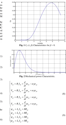
The simulation of the power coefficient and the mechanical power is shown in Figs. 1 and 2 respectfully.

3 The Model of DFIG

In this section, the Park model of the doubly fed induction generator is the most used [9-12]. The equations of voltages and fluxes for the DFIG rotor and stator in Park reference frame are given by:

0 1 2 3 4 5 6 7 8

0 0.05 0.1 0.15 0.2 0.25 0.3 0.35 0.4 0.45

Cp

Lambda

Fig. 1 Cp (λ, ß) Characteristics for ß = 0.

10 20 30 40 50 60 70 80 90 100

0 500 1000 1500 2000 2500

Wind speed v (m/s)

M

e

c

h

a

n

ic

a

l

p

o

w

e

r

P

m

(W

)

Fig. 2 Mechanical power Characteristic.

ds s ds ds s qs qs s qs qs s ds dr r dr dr r qr qr r qr qr r dr

d

V R I

dt d

V R I

dt d

V R I

dt d

V R I

dt

  

 _ _ _

 

 _ _ _

 

 _ _ _

 

   



(8)

ds s ds dr qs s qs qr dr r dr ds qr r qr qs

L I MI

   

 



 _ _



 _ _



 _ _



(9)

The rotor and stator angular velocities are linked by the following relation:

s w r

w  w (10)

where, w: is the mechanical pulsation, ws: is the

electrical pulsation of the stator, and wr is the pulsation

of the rotor.

The mechanical equation of the DFIG is:

e r

d

T T J f

dt 

    (11)

where, Tr is the load torque, J is the inertia, f is the

viscous friction coefficient, p is the number of pole

(3)

pairs.

The torque can be written as follows:

3

( )

2 dr qs qr ds

e

s

M

T p I I

L  

  (12)

The power equations are defined as:

3

( )

2 3

( )

2

s ds ds qs qs s qs ds ds qs

P V I V I

Q V I V I

  

 

 _ _



(13)

4 NPWM Strategy

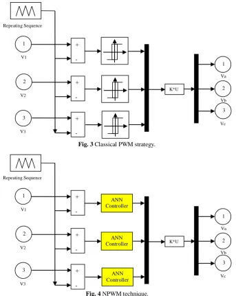
Pulse-width modulation, is a modulation strategy used to encode a message into a pulsing signal. The PWM strategy uses a rectangular pulse wave whose pulse width is modulated resulting in the variation of the average value of the waveform. The block diagram of the two-level PWM technique is presented in Fig. 3.

This strategy gives more THD value of rotor current, electromagnetic torque ripple, active and reactive power ripples of the DFIG-based wind turbine systems [13]. To minimize the THD value, torque ripple, reactive power ripple, active power ripple, and to increase the maximum amplitude fundamental of the output voltage of the two-level inverter, we have applied the neural pulse width modulation technique.

The principle of neural pulse width modulation technique is similar to traditional PWM strategy. The difference results in using a neural controller to replace the hysteresis comparators. As shown in Fig. 4. However, the NNs are part of the family of statistical learning methods inspired by the biological nervous system and are used to estimate and approximate functions that depend only on a large number of inputs [14]. On the other hand, the NN controller contains 3 layers: output layers, input layers and hidden layers. Each layer is composed of several neurons [15].

Fig. 3 Classical PWM strategy.

Fig. 4 NPWM technique. Repeating Sequence

Vc Va

Vb

+ -

1

2

3

K*U

1

2

3

V1

V2

V3

Repeating Sequence

Vc Va

Vb

+ -

1

2

3

K*U

1

2

3

V1

V2

V3

ANN Controller

(4)

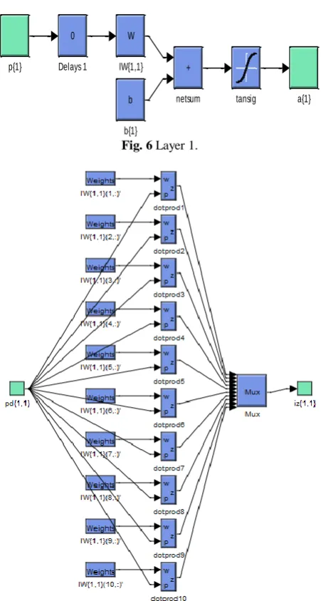
The structure of the NN controllers used to perform the PWM strategy is an ANN with one linear input node, 8 neurons in the hidden layer, and one neuron in the output layer. As shown in Fig. 5. The ANN controller is composed of two layers, Layer 1 (Fig. 6) and Layer 2 (Fig. 8). The training used is that of the retropropagation of Levenberg-Marquardt (LM). On the other hand, the parameters of the LM algorithm is shown in Table 1. On the other hand, the block diagram of the hidden layer of the neural controller is shown in Fig. 7.

5 Neuro-Sliding Mode Controller

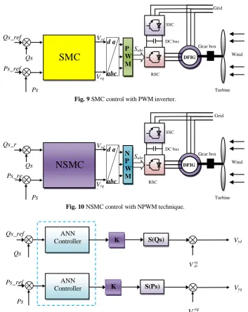
In what follows, a neuro-sliding mode controller is proposed to regulate the reactive and active power of a DFIG-based WTSs. However, the SMC control is one of the nonlinear strategies [16]. This strategy based on the theory of VSCS (variable structure control systems). On the other hand, this strategy is widely used for AC machine and the robustness is the best advantage of an SMC control. Nevertheless, this strategy has a huge disadvantage, which is the chattering phenomenon caused by the discontinuous control action. The SMC control with two-level PWM strategy, which is designed to control the reactive and stator active power of the doubly fed induction generator is shown in Fig. 9. Various control techniques have been proposed to reduce the chattering phenomenon of SMC control. The most used technique is SMC based on Fuzzy logic (FL)

controller and second-order sliding mode

controller (SOSMC). In [17], Fuzzy sliding mode controller (FSMC) was designed to control the reactive and active powers of a DFIG. A fuzzy controller and SOSMC are combined to regulate the active and reactive powers of DFIG-based WTSs [18]. In this paper, we propose a NSMC strategy to control the active and reactive stator power of a doubly fed induction generator-based wind energy conversion system. However, neural network is a technology based on engineering experience and observations. In NNs, an exact mathematical model is not necessary and is simple to implement compared to the classical techniques. In the SMC control, the control vector is imposed as follows:

eq n dq dq dq

V V V (14)

The equivalent control vector Veq_{can be expressed as}

[17]:

Output a{1}

Process Output 1 Process Input 1

Layer 2 Layer 1

a{1} Input

Fig. 5 Block diagram of the NN controller.

a{1} tansig

+

netsum b

b{1} W

IW{1,1} 0

Delays 1 p{1}

Fig. 6 Layer 1.

Fig. 7 Block diagram of the IW for layer 1.

a{2} purelin

+

netsum b

b{2} W

LW{2,1} 0

Delays 1 a{1}

Fig. 8 Layer 2.

Table 1 Parameters of the LM for hysteresis comparators.

Parameters of the LM Values

Number of hidden layers 8

TrainParam.Lr 0.005

TrainParam.show 50

TrainParam.eposh 1000

Coefficient of acceleration of convergence (mc)

0.9

TrainParam.goal 0

TrainParam.mu 0.9

Functions of activation Tensing, Purling, gensim

(5)

2 2

2

r r

eq s s

r dr s s r qr s

dr sref

s s

s

s s

eq

r qr r dr

qr sref s

s s

s

M M

L L

M

L _Q _g L

V R I L w L I w

M w L M

MV

L _P _g M _g

V R I w L I

M

V L L



 _ _

 _ _

    _  _ 

 _ _



 _ _

    _  _ 

  



(15)

n dq

V is the saturation function defined by:

. ( )

n

dq K sat dq

V   S (16)

where K determines the ability of overcoming the chattering.

The SMC will exist only if the following condition is met:

. 0

S S (17)

One way to improve SMC controller performance is to combine it with NN to form neuro-sliding mode

controller. The design of an SMC incorporating neural controller help in achieving reduced chattering phenomenon, powers ripples, distortion harmonic of rotor current, simple control, easy to implement and robustness against disturbances and nonlinearities. However, the NSMC is a modification of the SMC, where the switching controller term sat(S(x)), has been replaced by a neural control input as given below.

eq com Neural dq dq dq

V V V (18)

Fig. 10 represents the NSMC technique of a doubly fed induction generator driven by a two-level NPWM technique.

The proposed NSMC technique, which is designed to control the active and stator reactive powers of the doubly fed induction generator, is shown in Fig. 11.

Fig. 9 SMC control with PWM inverter.

Fig. 10 NSMC control with NPWM technique.

Fig. 11 Block diagram of the NSMC. Qs_ref

V

eqqr

Vrd *

Vrq * Ps_ref

Qs

Ps

+ -

+ _-

- ₊

ANN Controller

K

ANN

Controller - ₊ Veqdr

K

S(Ps) S(Qs)

Ps Qs_r ef

Grid

Turbine Wind Sabc

DC bus

DFIG

RSC

Vrd *

Vrq *

abc d q

Qs

N P W M

+ -

Ps_re f

NSMC

SSC

Gear box Ps

Qs_ref

Grid

Turbine Ps_ref

Wind Sabc

DC bus

DFIG

RSC

Vrd *

Vrq *

abc d q

Qs

P W M

+ -

+ _-

SMC

SSC

Gear box

(6)

The construction of the NN controller to realize the SMC control applied to DFIG adequately was a NN controller with one linear input node, 8 neurons in the hidden layer, and one neurone in the output layer, as shown in Fig. 12.

The convergence of the network in summer obtained by using the value of the parameters grouped in Table 2. The block diagram of the hidden layer for the neural controller is shown in Fig. 13.

Output a{1}

Process Output 1 Process Input 1

Layer 2 Layer 1

a{1} Input

Fig. 12 Block diagram of the ANN controller.

Table 2 Parameters of the LM for switching controller.

Parameters of the LM Values

Number of hidden layer 08

TrainParam.Lr 0.005

TrainParam.show 50

TrainParam.eposh 1000

Coeff of acceleration of convergence (mc)

0.9

TrainParam.goal 0

TrainParam.mu 0.9

Functions of activation Tensing, Purling, gensim

Fig. 13 Block diagram of the hidden layer.

6 Simulation Results

In this section, simulations are investigated with a 1.5MW generator connected to a 398V/50Hz grid. The machine parameters are presented in the Table 3 (see Appendix 1). The proposed control schemes will be tested and compared to two different configurations: robustness against parameters variations and reference tracking.

6.1 Reference Tracking Test (RTT)

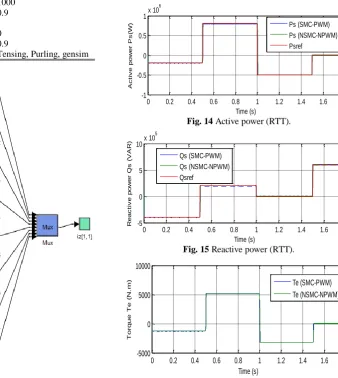
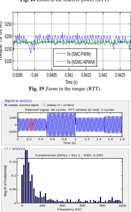
Figs. 14-21 show the obtained simulation results. For the proposed control schemes, the active and stator reactive power track almost perfectly their references

values. Moreover, the NSMC-NPWM control

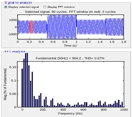
minimized the powers ripples compared to the SMC-PWM control (See Figs. 17-19). On the other hand, Figs. 20-21 shows the harmonic spectrums of one phase rotor current of the doubly fed induction generator obtained using Fast Fourier Transform technique for NSMC-NPWM and SMC-PWM one respectively. It can be clearly observed that the THD is reduced for NSMC-NPWM control technique (THD = 0.13%) when compared to SMC-PWM (THD = 0.33%).

0 0.2 0.4 0.6 0.8 1 1.2 1.4 1.6 1.8 -1

-0.5 0 0.5

1x 10

6

Time (s)

A

c

ti

v

e

p

o

w

e

r

P

s

(W

)

0 0.2 0.4 0.6 0.8 1 1.2 1.4 1.6 1.8 -5

0 5 10x 10

5

Time (s)

R

e

a

c

ti

v

e

p

o

w

e

r

Q

s

(

V

A

R

)

0 0.2 0.4 0.6 0.8 1 1.2 1.4 1.6 1.8 -2000

-1000 0 1000 2000

Time (s)

S

ta

to

r

c

u

rr

e

n

t

(A

)

0 0.2 0.4 0.6 0.8 1 1.2 1.4 1.6 1.8 -5000

0 5000 10000

Time (s)

T

o

rq

u

e

T

e

(

N

.m

)

Ps (SMC-PWM) Ps (NSMC-NPWM) Psref

Qs (SMC-PWM) Qs (NSMC-NPWM) Qsref

Te (SMC-PWM) Te (NSMC-NPWM)

Fig. 14 Active power (RTT).

0 0.2 0.4 0.6 0.8 1 1.2 1.4 1.6 1.8 -1

-0.5 0 0.5

1x 10

6

Time (s)

A

c

ti

v

e

p

o

w

e

r

P

s

(W

)

0 0.2 0.4 0.6 0.8 1 1.2 1.4 1.6 1.8 -5

0 5 10x 10

5

Time (s)

R

e

a

c

ti

v

e

p

o

w

e

r

Q

s

(

V

A

R

)

0 0.2 0.4 0.6 0.8 1 1.2 1.4 1.6 1.8 -2000

-1000 0 1000 2000

Time (s)

S

ta

to

r

c

u

rr

e

n

t

(A

)

0 0.2 0.4 0.6 0.8 1 1.2 1.4 1.6 1.8 -5000

0 5000 10000

Time (s)

T

o

rq

u

e

T

e

(

N

.m

)

Fig. 15 Reactive power (RTT).

0 0.2 0.4 0.6 0.8 1 1.2 1.4 1.6 1.8

-1 -0.5 0 0.5

1x 10

6

Time (s)

A

c

ti

v

e

p

o

w

e

r

P

s

(W

)

0 0.2 0.4 0.6 0.8 1 1.2 1.4 1.6 1.8

-5 0 5 10x 10

5

Time (s)

R

e

a

c

ti

v

e

p

o

w

e

r

Q

s

(

V

A

R

)

0 0.2 0.4 0.6 0.8 1 1.2 1.4 1.6 1.8

-2000 -1000 0 1000 2000

Time (s)

S

ta

to

r

c

u

rr

e

n

t

(A

)

0 0.2 0.4 0.6 0.8 1 1.2 1.4 1.6 1.8

-5000 0 5000 10000

Time (s)

T

o

rq

u

e

T

e

(

N

.m

)

Fig. 16 Electromagnetic torque (RTT).

(7)

0.762 0.763 0.764 0.765 0.766 0.767 0.768 0.769 0.77 7.9

7.95 8 8.05 8.1

x 105

Time (s) A c ti v e p o w e r P s (W )

0.917 0.918 0.919 0.92 0.921 0.922 0.923 0.924 0.925 1.95

2 2.05

2.1x 10

5 Time (s) R e a c ti v e p o w e r Q s ( V A R )

0 0.2 0.4 0.6 0.8 1 1.2 1.4 1.6 1.8

-2000 -1000 0 1000 2000 Time (s) S ta to r c u rr e n t (A )

0.8395 0.84 0.8405 0.841 0.8415 0.842 0.8425 5100 5150 5200 5250 Time (s) T o rq u e T e ( N .m ) Ps (SMC-PWM) Ps (NSMC-NPWM) Psref Qs (SMC-PWM) Qs (NSMC-NPWM) Qsref Te (SMC-PWM) Te (NSMC-NPWM)

Fig. 17 Zoom in the active power (RTT).

0.762 0.763 0.764 0.765 0.766 0.767 0.768 0.769 0.77 7.9

7.95 8 8.05 8.1

x 105

0.917 0.918 0.919 0.92 0.921 0.922 0.923 0.924 0.925 1.95

2 2.05

2.1x 10

0 0.2 0.4 0.6 0.8 1 1.2 1.4 1.6 1.8

-2000 -1000 0 1000 2000 Time (s) S ta to r c u rr e n t (A )

0.8395 0.84 0.8405 0.841 0.8415 0.842 0.8425 5100 5150 5200 5250 Time (s) T o rq u e T e ( N .m ) Ps (SMC-PWM) Ps (NSMC-NPWM) Psref Qs (SMC-PWM) Qs (NSMC-NPWM) Qsref Te (SMC-PWM) Te (NSMC-NPWM)

Fig. 18 Zoom in the reactive power (RTT).

0.762 0.763 0.764 0.765 0.766 0.767 0.768 0.769 0.77 7.9

7.95 8 8.05 8.1

x 105

Time (s) A c t iv e p o w e r P s ( W )

0.917 0.918 0.919 0.92 0.921 0.922 0.923 0.924 0.925 1.95

2 2.05

2.1x 10

5 Time (s) R e a c t iv e p o w e r Q s ( V A R )

0 0.2 0.4 0.6 0.8 1 1.2 1.4 1.6 1.8 -2000 -1000 0 1000 2000 Time (s) S t a t o r c u r r e n t ( A )

0.8395 0.84 0.8405 0.841 0.8415 0.842 0.8425 5100 5150 5200 5250 Time (s) T o r q u e T e ( N . m ) Ps (SMC-PWM) Ps (NSMC-NPWM) Psref Qs (SMC-PWM) Qs (NSMC-NPWM) Qsref Te (SMC-PWM) Te (NSMC-NPWM)

Fig. 19 Zoom in the torque (RTT).

0 0.2 0.4 0.6 0.8 1 1.2 1.4 1.6 1.8 -1000

0 1000

Selected signal: 90 cycles. FFT window (in red): 3 cycles

Time (s)

0 200 400 600 800 1000 0

0.05 0.1 0.15

Frequency (Hz)

Fundamental (50Hz) = 911.2 , THD= 0.33%

M ag ( % o f F un da m en ta l)

Fig. 20 THD of rotor current for SMC-PWM control (RTT).

6.2 Robustness Test (RT)

In the following section, the nominal value of the Rr

and Rs is doubled, the values of inductances Ls, M, and

Lr are halfed. Simulation results are presented in

Figs. 22-27 and Figs. 28-29. As shown, these variations present a clear effect on the active power, reactive power, rotor current and electromagnetic torque. However, the effect appears more important for the SMC-PWM control technique compared to NSMC-NPWM control (see Figs. 25-27). On the other hand, the THD value of rotor current in the NSMC-NPWM has been significantly minimized. Table 4 shows the comparative analysis of THD value. Thus it can be concluded that the NSMC-NPWM control technique is more robust than the SMC-PWM control.

0 0.2 0.4 0.6 0.8 1 1.2 1.4 1.6 1.8 -1000

0 1000

Time (s)

0 200 400 600 800 1000 0 0.02 0.04 0.06 0.08 0.1 0.12 0.14 Frequency (Hz) Fundamental (50Hz) = 914.9 , THD= 0.13%

Fig. 21 THD of rotor current for NSMC-NPWM control (RTT).

Table 4 Comparative analysis of THD value (RT). THD [%]

SMC-PWM NSMC-NPWM

Rotor current 0.67 0.25

0 0.2 0.4 0.6 0.8 1 1.2 1.4 1.6 1.8 -1

-0.5 0 0.5

1x 10

6 Time (s) A c ti v e p o w e r P s (W )

0 0.2 0.4 0.6 0.8 1 1.2 1.4 1.6 1.8 -5

0 5 10x 10

0 0.2 0.4 0.6 0.8 1 1.2 1.4 1.6 1.8 -2000 -1000 0 1000 2000 Time (s) S ta to r c u rr e n t (A )

0 0.2 0.4 0.6 0.8 1 1.2 1.4 1.6 1.8 -5000 0 5000 10000 Time (s) T o rq u e T e ( N .m ) Ps (SMC-PWM) Ps (NSMC-NPWM) Psref Qs (SMC-PWM) Qs (NSMC-NPWM) Qsref Te (SMC-PWM) Te (NSMC-NPWM) Fig. 22 Active power (RT).

0 0.2 0.4 0.6 0.8 1 1.2 1.4 1.6 1.8 -1

-0.5 0 0.5

1x 10

6 Time (s) A c ti v e p o w e r P s (W )

0 0.2 0.4 0.6 0.8 1 1.2 1.4 1.6 1.8 -5

0 5 10x 10

0 0.2 0.4 0.6 0.8 1 1.2 1.4 1.6 1.8 -5000 0 5000 10000 Time (s) T o rq u e T e ( N .m ) Ps (SMC-PWM) Ps (NSMC-NPWM) Psref Qs (SMC-PWM) Qs (NSMC-NPWM) Qsref Te (SMC-PWM) Te (NSMC-NPWM)

Fig. 23 Reactive power (RT).

(8)

Sliding Mode with Neural Network Regulator for DFIG Using … H. Benbouhenni

0 0.2 0.4 0.6 0.8 1 1.2 1.4 1.6 1.8 -1 -0.5 0 Time (s) A c t iv e p o w e r P

0 0.2 0.4 0.6 0.8 1 1.2 1.4 1.6 1.8 -5 0 5 Time (s) R e a c t iv e p o w e r Q

0 0.2 0.4 0.6 0.8 1 1.2 1.4 1.6 1.8 -5000 0 5000 10000 Time (s) T o r q u e T e ( N . m ) Psref Qsref Te (SMC-PWM) Te (NSMC-NPWM)

Fig. 24 Electromagnetic torque (RT).

0.31 0.315 0.32 0.325

-2.1 -2 -1.9 -1.8

x 105

1.285 1.29 1.295 1.3 1.305

-2 -1 0 1 2

x 104

Time (s) R e a c ti v e p o w e r Q s ( V A R )

1.63 1.635 1.64 1.645 1.65 -50 0 50 100 Time (s) T o rq u e T e ( N .m ) Ps (SMC-PWM) Ps (NSMC-NPWM) Psref Qs (SMC-PWM) Qs (NSMC-NPWM) Qsref Te (SMC-PWM) Te (NSMC-NPWM) Fig. 25 Zoom in the active power (RT).

0.31 0.315 0.32 0.325

-2.1 -2 -1.9 -1.8

x 105

1.285 1.29 1.295 1.3 1.305 -2

-1 0 1 2

x 104

Time (s) R e a c ti v e p o w e r Q s ( V A R )

1.63 1.635 1.64 1.645 1.65 -50 0 50 100 Time (s) T o rq u e T e ( N .m ) Ps (SMC-PWM) Ps (NSMC-NPWM) Psref Qs (SMC-PWM) Qs (NSMC-NPWM) Qsref Te (SMC-PWM) Te (NSMC-NPWM)

Fig. 26 Zoom in the reactive power (RT).

0.31 0.315 0.32 0.325

-2.1 -2 -1.9 -1.8

x 105

Time (s) A c t iv e p o w e r P s ( W )

1.285 1.29 1.295 1.3 1.305 -2

-1 0 1 2

x 104

Time (s) R e a c t iv e p o w e r Q s ( V A R )

1.63 1.635 1.64 1.645 1.65 -50 0 50 100 Time (s) T o r q u e T e ( N . m ) Ps (SMC-PWM) Ps (NSMC-NPWM) Psref Qs (SMC-PWM) Qs (NSMC-NPWM) Qsref Te (SMC-PWM) Te (NSMC-NPWM)

Fig. 27 Zoom in the electromagnetic torque (RT).

0 0.2 0.4 0.6 0.8 1 1.2 1.4 1.6 1.8 -1000

0 1000

Time (s)

0 200 400 600 800 1000 0

0.05 0.1 0.15

Frequency (Hz)

Fig. 28 THD of rotor current for SMC-PWM control (RT).

0 0.2 0.4 0.6 0.8 1 1.2 1.4 1.6 1.8 -1000

0 1000

Time (s)

0 200 400 600 800 1000 0

0.05 0.1 0.15

Frequency (Hz)

Fig. 29 THD of rotor current for NSMC-NPWM control (RT).

7 Conclusion

In this article, we presented the sliding mode control with the neural network of the stator reactive and active powers of the doubly fed induction generator supplied by neural pulse width modulation techniques at two-level.

This study presents a control strategy for a doubly fed induction generator based wind turbine systems using the SMC and NSMC with a different modulation technique (PWM, NPWM). The simulation results show that the NSMC control with NPWM is an excellent solution for doubly fed induction generator based wind turbine. The results of the simulation clearly show good performances with the NPWM technique. Indeed, while comparing with traditional PWM technique, the

neuro-sliding mode control with NPWM method is faster and more robust in the various operating processes of the engine (tracking tests and robustness tests).

Appendix 1

Table 3 The DFIG Parameters.

Parameters Rated Value Unit

P 1.5 MW

Vs 398/690 V

Fs 50 Hz

P 2

Rs 0.012 Ω

Rr 0.021 Ω

Ls 0.0137 H

Lr 0.0136 H

M 0.0135 H

J 1000 Kg m2

f 0.0024 Nm/s

(9)

Iranian Journal of Electrical and Electronic Engineering, Vol. 15, No. 3, September 2019 419 References

[1] Y. Bekakra and D. B. Attous, “Comparison study between SVM and PWM inverter in sliding mode control of active and reactive power control of a DFIG for variable speed wind energy,” International Journal of Renewable Energy Research, Vol. 2, No. 3, pp. 471–476, 2012.

[2] H. Benbouhenni, “Fuzzy second order sliding mode controller based on three-level fuzzy space vector modulation of a DFIG for wind energy conversion systems,” Majlesi Journal of Mechatronic Systems, Vol. 7, No. 3, 2018.

[3] Z. Boudjema, A. Meroufel, Y. Djerriri, and E. Bounadja, “Fuzzy sliding mode control of a doubly fed induction generator for wind energy conversion,” Carpathian Journal of Electronic and Computer Engineering, Vol. 6, No. 2, pp. 7–14, 2013.

[4] A. Yahdou, B. Hemici, and Z. Boudjema, “Second order sliding mode control of a dual-rotor wind turbine system by employing a matrix converter,” Journal of Electrical Engineering, Vol. 16, No. 4, pp. 1–11, 2016.

[5] H. Benbouhenni, Z. Boudjema, and A. Belaidi, “Neuro-second order sliding mode control of a DFIG supplied by a two-level NSVM inverter for wind turbine system,” Iranian Journal of Electrical and Electronic Engineering, Vol. 14, No. 4, pp. 362–373, 2018.

[6] A. Medjber, A. Moualdia, A. Mellit, M. A. Guessoum, “Comparative study between direct and indirect vector control applied to a wind turbine equipped with a double-fed asynchronous machine Article,” International Journal of Renewable Energy Research, Vol. 3, No. 1, pp. 88–93, 2013.

[7] N. Khemiri, A. Khedher, and M. F. Mimouni, “Wind energy conversion system using DFIG controlled by backstepping and sliding mode strategies,” International Journal of Renewable Energy Research, Vol. 2, No.3, pp. 422–435, 2012.

[8] S. A. Nowdeh, M. Chitsaz, and S. Khanabdal, “Evaluation of 1-phase, 3-phase and hightning faults on wind frams using EMTP-RV,” Majlesi Journal of Electrical Engineering, Vol. 8, No. 1, pp. 53–61, 2014.

[9] A. Nazari and H. Heydari, “Direct power control

topologies for DFIG-based wind plants,”

International Journal of Computer and Electrical Engineering, Vol. 4, No. 4, pp. 475–479, 2012.

[10]A. Fekik, H. Denoun, N. Benamrouche,

N. Benyahia, and M. Zaouia, ”A fuzzy–logic based controller for three phase PWM rectifier with voltage oriented control strategy,” International Journal of Circuits, Systems and Signal Processing, Vol. 9, pp. 412–419, 2015.

[11]D. Phan and S. Yamamoto, ”Maximum energy output of a DFIG wind turbine using an improved MPPT-curve method,” Energies, Vol. 8, pp. 11718– 11736, 2015.

[12]R. Pourebrahim, S. Tohidi, and A. Younesi, “Sensorless model reference adaptive control of DFIG by using high frequency signal injection and fuzzy logic control,” Iranian Journal of Electrical and Electronic Engineering, Vol. 14, No. 1, pp.11– 21, 2018.

[13]H. Benbouhenni, Z. Boudjema, and A. Belaidi, “DFIG-based WT system using FPWM inverter,” International Journal of Smart Grid, Vol. 2, No. 3, pp. 142–154, 2018.

[14]A. Idir and M. Kidouche, “Direct torque control of three phase induction motor drive using fuzzy logic controllers for low torque ripple,” Proceedings Engineering & Technology, Vol. 2, pp. 78–83, 2013.

[15]H. Benbouhenni, “Seven-level direct torque control of induction motor based on artificial neural networks with regulation speed using fuzzy PI controller,” Iranian Journal of Electrical and Electronic Engineering, Vol. 14, No.1, pp.85–94, 2018.

[16]B. Karima and A. Boukhelifa, “Output power control of a variable wind energy conversion system,” Revue Roumaine Des Sciences Techniques-Serie Electrotechnique Et Energetique, Vol. 62, No. 2, pp. 197–202, 2017.

[17]S. A. E. Ardjoun and M. Abid, “Fuzzy sliding mode control applied to a doubly fed induction generator for wind turbines,” Turkish Journal of Electrical Engineering & Computer Sciences, Vol. 23, pp. 1673–1686, 2015.

[18]Z. Boudjema, R. Taleb, and A. Yahdou, “A new DTC scheme using second order sliding mode and fuzzy logic of a DFIG for wind turbine system,” International Journal of Advanced Computer Science and Applications, Vol. 7, No. 8, pp.49–56, 2016.

H. Benbouhenni was born in Chlef, Algeria. He is a Ph.D. student in the Department of Electrical Engineering at the ENPO-MA, Oran, Algeria. He received a M.A. degree in Automatic and Informatique Industrial in 2017. His research activities include the application of robust control in the wind turbine power systems.

© 2019 by the authors. Licensee IUST, Tehran, Iran. This article is an open access article distributed unde r the terms and conditions of the Creative Commons Attribution-NonCommercial 4.0 International (CC BY-NC 4.0) license (https://creativecommons.org/licenses/by-nc/4.0/).