Volume 10, Number 4, pp. 337–345. http://www.scpe.org c 2009 SCPE
VECTORIZED SOLUTION OF ODES IN MATLAB
L. F. SHAMPINE∗
Abstract. Vectorization is very important to the efficiency of computation in the popular problem-solving environment Matlab. It is shown that a class of Runge-Kutta methods investigated by Milne and Rosser that compute a block of new values at each step are well-suited to vectorization. Local error estimates and continuous extensions that require no additional function evaluations are derived. A (7,8) pair is derived and implemented in a programBV78 that is shown to perform quite well when compared to the well-knownMatlabODE solverode45which is based on a (4,5) pair.
Key words: Matlab, vectorization, ordinary differential equations, initial value problems
1. Introduction. Matlab is a problem-solving environment (PSE) that is in very wide use. A suite of programs for solving the initial value problem (IVP) for ordinary differential equations (ODEs) in this PSE is developed in [11]. As illustrated there, both algorithms and coding practices must take into account that the costs of certain computations inMatlab are quite different from the costs in general scientific computation. Indeed, all the programs inMatlabfor approximating Rb
af(x)dx require that evaluation of the integrand be coded to accept a vector [x1, x2, . . . , xk] and return a vector [f(x1), f(x2), . . . , f(xk)]. That is because the cost of evaluating the integrand for all these arguments in one call with an array argument is generally not much greater than the cost of a call with a single argument. There are two reasons for this. One is that the overhead of a call is relatively expensive and the other is that skillful use of array operations and vectorized built-in functions generally allows an integrand to be evaluated very efficiently forkarguments simultaneously. When evaluation of the integrand is coded in this way, the function is said to be “vectorized”. In this paper we consider how vectorization might be exploited when solving numerically a system ofnfirst-order ODEs
y′=f(t, y) (1.1)
on an interval [t0, tf] with initial value y0 = y(t0). There are already some examples of this in Matlab. When solving stiff IVPs, it is necessary to form Jacobian matricesJ(t, y) from time to time. By default these Jacobians are approximated by finite differences. If the Jacobian is dense, J(t0, y0) is approximated using values off(t0, ym) forn vectors{y1, y2, . . . , yn}that are “close” to y0. Users are encouraged to vectorize the computation so that whent0 and a matrix with columns{y1, . . . , yn} are input, the function will compute and return the corresponding {f(t0, y1), . . . , f(t0, yn)} as columns in a matrix. If full advantage is taken of array operations, the Jacobian can often be approximated at a cost not much greater than the cost of evaluatingf for a singleym. Kierzenka [5, 10] recognized that when solving boundary value problems (BVPs) with collocation methods, the cost of solving the associated nonlinear algebraic equations could be reduced very substantially if evaluation off(t, y) was vectorized so that for{t1, t2, . . . , tk} given as entries in a vector and{y1, y2, . . . , yk} given as columns in a matrix, the function returns{f(t1, y1), . . . , f(tk, yk)}as columns in a matrix. Because the argumenty is generally a vector when solving ODEs, we use in this paper the term “array evaluation” off to distinguish the evaluation off(t, y) with vectortand matrixy from an evaluation with a scalartand vectory. To compute starting values for multistep methods, Milne [8] suggested a scheme that is described nowadays as a block Runge-Kutta (RK) method. The scheme starts with an approximationy0toy(t0) and then computes simultaneously a block of approximationsy1, y2, . . . , yr at points t0+h, t0+ 2h, . . . , t0+rh. Later Rosser [9] proposed an explicit variant of these formulas. He uses simple (functional) iteration to evaluate the implicit formulas, but does a fixed number of iterations so as to obtain an explicit RK method. Rosser argues that these explicit block RK methods require many evaluations off at each step, but when it is appreciated thatr new values are formed, the cost per new value is lower than for conventional schemes of moderate to high order. The methods never caught on, but we observe here that they are quite attractive inMatlab because they are so well suited to vectorization. The key observation is that each iteration requires only one array evaluation of the function. With this a high order can be obtained with a remarkably small number of (array) function evaluations. In this paper we show that it is easy to estimate the local error without additional function evaluations. Using this result, we implemented the scheme studied in detail by Rosser as a (5,6) pair in a programR56. We also
∗Mathematics Department, Southern Methodist University, Dallas, TX 75275. E-mail:[email protected]
show that a continuous extension is available without additonal function evaluations. Appreciating that the advantages of vectorization are greater at higher order, we derived formulas analogous to R(5,6) for a (7,8) pair and a corresponding continuous extension. TheBV78program that implements these formulas was substantially more efficient thanR56, so we give our attention primarily to the (7,8) pair. We compareBV78to theMatlab
ode45solver because the documentation of the PSE recommends ode45for non-stiff problems that are to be solved for moderate to stringent accuracies. In§4 we see that the (7,8) pair has stability comparable to that of the (4,5) pair implemented inode45. In§5 we find thatBV78solves a wide range of standard test problems for a wide range of tolerances in about one third the time required byode45.
2. Explicit RK Pairs in Matlab. When the ODE Suite [11] was originally conceived, the authors were very interested in implementing one of the effective (7,8) pairs derived by Fehlberg, Dormand and Prince, and Verner. The main reason this was not done is the cost of a continuous extension for the pair. To be concrete, we discuss in this article a particularly efficient pair of 13 stages due to Verner [13]. He derived continuous extensions of orders 7 and 8 that require 3 and 4 extra stages, respectively. In Matlab it is typical that a user plot the solution. The (7,8) pairs take rather long steps, long in the sense that a solution can change substantially over the span of the step. The same is true of the (4,5) pair derived by Dormand and Prince [3] that is implemented in ode45, though to a lesser degree. This pair, which is known as DOPRI5, is a 7 stage pair, but it is FSAL, meaning that if the step is a success, the last stage of the step can be used as the first stage of the next step. Most steps are successful, so this pair generally costs little more than 6 stages per step. Because solution values at mesh points alone often do not provide a satisfactory plot, theode45solver evaluates a continuous extension to obtain approximate solutions at some additional points equally spaced in the span of each step. Although we might have preferred a continuous extension of order 5, it would require extra function evaluations. These function evaluations are made at every step in typical use of the solver, which increases the cost of the pair by a relatively large amount. An interpolant of order 4 is implemented inode45because it is an adequate approximation that costs no extra function evaluations. The extra stages for interpolation with the popular (7,8) pairs increase the cost so much at every step in typical use of a Matlab ODE solver that we decided not to provide anode78. The fact that the typical problem is solved to only moderate accuracy in
Matlab also influenced this decision. For the sake of completeness, we note that for the relatively low order BS(2,3) pair [1] implemented in ode23, values at mesh points alone generally do provide a satisfactory plot. Accordingly, this solver does not evaluate the continuous extension to obtain additional approximations in the span of each step. Even if it did, this would be inexpensive because the continuous extension requires no extra function evaluations.
3. Block RK Methods. A difficulty with multistep methods is to compute somehow starting values. Milne [8] suggested a scheme that is described nowadays as a block Runge-Kutta (RK) method. The method starts with an approximationy0 to the solution att0 and then computes simultaneously a block of approxima-tionsy1, y2, . . . , yr at pointst0+h, t0+ 2h, . . . , t0+rh. We prefer to rescale so as to view the method as an implicit RK formula that steps fromt0tot0+hand in the course of the step forms accurate approximations at points equally spaced in the span of the step, namelyt0+h/r, t0+ 2h/r, . . . , t0+h. The formulas are commonly derived by using an integrated form of the ODEs and replacing the integrals with quadrature formulas. With equally spaced points the quadrature schemes are of Newton-Cotes type, so the block RK method is also said to be of Newton-Cotes type. For our purposes it will be more convenient to derive the formulas by collocation. In this approach a polynomialP(t) withP(t0) =y0 is to collocate at equally spaced pointstj =t0+jh/r for
j= 0,1, . . . , r. With the notationyj =P(tj) andfj=f(tj, yj), the resulting formulas have the form
y1= (y0+h A1,0f0) +h[A1,1f1+. . .+A1,rfr]
y2= (y0+h A2,0f0) +h[A2,1f1+. . .+A2,rfr] ..
. =...
yr= (y0+h Ar,0f0) +h[Ar,1f1+. . .+Ar,rfr]
We remark that if we denote these equations as Eq1, Eq2, . . . , Eqr, then combining and replacing them with
order r+ 1. A familiar example is the trapezoidal rule which hasr = 1 and global order 2. It is also shown in [14] that ifr is even, the value at the end of the step has a higher local order than at intermediate points, namelyr+ 3, hence the method is of global orderr+ 2. Clippinger and Dimsdale developed the formulas for the caser= 2, see [12] for details. When written in the form of an implicit RK method, it is found that this is a familiar method known as the three point Lobatto or Simpson method. An important reason for choosing it as the basic formula of the BVP solverbvp4c[5] is that it has global order 4, the one intermediate value is also of order 4, and a natural continuous extension is uniformly of order 4. Milne [8] provides an example known as Method IV which hasr= 4. For that example the intermediate values are all of local order 6 and the RK method is of global order 6.
Implicit RK methods have not been widely used to solve non-stiff IVPs because of the cost of evaluating the formulas. Rosser [9] takes a different approach. He starts an iteration for evaluating the implicit formulas, but does a fixed number of iterations so as to obtain an explicit RK method. The caser= 1 is a familiar example. If Euler’s method is used to form the first approximation toy1 and a single iteration of simple (functional) iteration is done, the resulting formula is an explicit RK formula of global order two known as Heun’s method. In the same way Rosser proposes starting with the locally second order approximationsyj[1] =y0+ (jh/r)f0 forj= 1, . . . , r. Simple iteration consists of first forming the fj[m]=f(tj, y[
m]
j ) and then computing they [m+1] j from
y[1m+1] = (y0+h A1,0f0) +h
h
A1,1f1[m]+. . .+A1,rfr[m]
i
y[2m+1] = (y0+h A2,0f0) +h
h
A2,1f1[m]+. . .+A2,rfr[m]
i
.. . =...
y[m+1]
r = (y0+h Ar,0f0) +h
h
Ar,1f[ m]
1 +. . .+Ar,rfr[m]
i
In connection with Milne’s Method IV, Rosser points out that each iteration raises the local order of the approximationsyj[m]by one (up to a maximum order determined by the order of the underlying implicit formula), so that after 5 iterations, they all have local order 6. When another iteration is done, the local order remains 6 at all the interior points, but the local error at the end of the step is increased to 7, resulting in a formula of global order 6. It is easily seen that this observation about the order of accuracy of the iterates is general—each iteration raises the local order of the approximations by one.
Rosser argues that these explicit block methods require many evaluations off at each step, but when it is appreciated that r new values are formed, the cost per new value is lower than for conventional schemes of moderate to high order. Vectorization changes completely our view of the cost of these explicit block RK methods. The key observation is that when the evaluation off is vectorized, we can formfj[m] forj= 1,2, . . . , r in a single call. Because of this a high order can be obtained with a remarkably small number of (array) function evaluations. Although Rosser did not take up any general ways of estimating the error, we noticed that this is easily done for block methods. Because each iterate raises the order by one, we not only have a result of global order 6 at the end of a step with Rosser’s method, we also have a result of global order 5. With it we have a (5,6) pair with a conventional local error estimate.
The block, vectorized Newton-Cotes formulas are very attractive as regards a continuous extension because the method is defined in terms of interpolating polynomials. Specifically, the values yj[m+1] are just P[
m](t j) for the polynomial P[m](t) that interpolates the value y
0 and the slopes f[ m]
j for j = 0,1. . . , r. This means that when we reach the m that provides the desired order, we already have available a continuous extension. We might remark that Rosser [9] does not consider this natural continuous extension, preferring instead to do Hermite interpolation on a subset of the new values. The BV78 solver we implemented shares the basic design of the ODE Suite. In particular, the default mode is for a user to supply the interval of integration. The solver then returns approximate solutions on a mesh that spans the interval. The BV(7,8) pair forms six new approximations equally spaced within each step. They are all returned by the solver. In our experiments these values have always provided a smooth graph, so this matter is handled rather more easily than inode45. Another mode is for a user to supply not only the interval, but also specific points where output is desired. The solvers then return approximate solutions at these points only. For efficiency the solvers choose the same step sizes for both modes of output and compute approximations at specific points in the span of a step by evaluating the continuous extension. Evaluation of the continuous extension to get output at specific points is coded as a nested function that is vectorized with respect to output points in the span of a step.
4. Stability. It is shown in [14] that the implicit block one-step methods defined by interpolatory formulas of Newton-Cotes type are A-stable for block sizesr= 1,2, . . . ,8. Of course, the stability regions of the explicit Runge-Kutta methods defined by evaluating such a formula with Euler’s method followed by a fixed number of simple iterations are all finite, but we might hope that the methods will at least have good stability. The lowest order case is the trapezoidal rule with r= 1. A single iteration leads to Heun’s method, which is a familiar two-stage, second-order explicit RK method. All such methods have the same region of absolute stability which is displayed as Figure 7.2 in Dormand [3]. It is reasonably large, which gives us hope that the BV(7,8) pair will inherit good stability from the underlying A-stable implicit RK formula. Figure 4.1 shows the stability regions of the two formulas of the BV(7,8) pair. Both regions are quite satisfactory as regards both size and shape. And, as these things go, the stability regions of the pair match pretty well. Figure 7.4 of [3] shows the stability regions of the DOPRI5 pair used inode45. The stability regions of the two pairs are comparable, but those of the BV(7,8) pair are uniformly somewhat bigger, especially in the direction of increasing imaginary part. On the other hand, the (7,8) pair costs 8 evaluations per step and the (4,5) pair only 6 for a successful step. However, this somewhat overstates the efficiency of the DOPRI5 pair because it is FSAL. This is less advantageous when stability is an issue because there are then many step failures in which case the pair costs 7 evaluations. All things considered, the stability of the BV(7,8) pair and the DOPRI5 pair may be fairly described as comparable.
Both formulas of Verner’s (7,8) pair have excellent stability and their regions are almost perfectly matched. Verner states that the average radius of the eighth order formula is 5.69. The typical solution of an IVP in
Matlabdisplays the solution graphically and for high order formulas it is necessary to produce some additional solution values in the span of each step so as to get a smooth graph. When used in this way, Verner’s pair costs 16 or 17 stages per step. The BV(7,8) pair costs 8 (array) evaluations per step and the interpolant costs no extra evaluations. Even if we assume that no interpolation is done, scaling the radius of the stability regions of Verner’s pair to the same number of evaluations as the BV(7,8) pair results in an equivalent radius of 5.69×8/13 = 3.50. This is quite a bit smaller than the average radius 4.66 of the eighth order formula of BV(7,8). It appears, then, that the BV(7,8) pair is rather more stable than Verner’s (7,8) pair provided that the cost of evaluatingf is a weak function of the number of arguments.
In §5 we describe some numerical experiments with BV78 and ode45applied to a test set of Krogh [6]. Details of the computations are provided in that section, but the problem K7 is pertinent here. The IVP
y′ =t(1−y) + (1−t)e−t, y(0) = 1
is to be solved on [0,50] with a pure absolute error control. The eigenvalue−t of the local Jacobian increases in magnitude as the integration proceeds, making the problem increasingly stiff. Figure 4.2 shows how much accuracy is achieved for a given number of function evaluations. In this no distinction is made between calling the function with one or six arguments. As we might have expected from the stability regions and costs per step, the two codes perform much the same. Table 5.1 shows that the same is true with respect to run times.
−5 −4 −3 −2 −1 0 0
0.5 1 1.5 2 2.5 3 3.5 4 4.5 5
Fig. 4.1.Stability regions for BV(7,8). Order 8 is the larger region.
2000 3000 4000 5000 6000 7000 8000 10−14
10−12 10−10 10−8 10−6 10−4 10−2 100
Number of function evaluations.
Tolerance
BV78 ode45
Fig. 4.2.K7 tests stability along the negative real axis.
10−100. Analytical solutions are available for all the problems except K9 and K10. Reference values for the two body problem K9 were obtained by solving accurately Kepler’s (algebraic) equation. Reference values for the restricted three body problem K10 were computed using ode113with the minimum relative error tolerance of 2.2×10⁻¹⁶and absolute error tolerance of 10−100. This should provide a solution accurate enough to compare the solvers for tolerances 10−2,10−3, . . . ,10−12. For some problems one or more of these tolerances was excluded from the comparison because one of the solvers had an error bigger than 1.
An important issue in comparing solvers is where they are to be compared. An approach that is typical of methods without continuous extensions is to measure the accuracy only at mesh points. Krogh specifies the points where the accuracy is to be measured. However, he specifies only a few points and as a consequence, quality solvers without continuous extensions are not much affected by output at these points. Our approach is more revealing and closer to the way solvers are used in Matlab. We compared the accuracy at 200 points equally spaced in the interval of integration. More precisely, we measured the maximum over the 200 points of the maximum relative or absolute error, as the case may be, in the components of the solution at each point. This tests not just the accuracy of the solver, but also the accuracy of the continuous extension. Furthermore, it tests the overhead of evaluating the continuous extension along with the overhead of the solver itself.
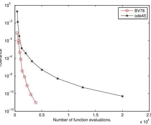
It is difficult to obtain consistent run times inMatlab. This is especially true when the run times are small in absolute terms,as they are for these test problems. We summed the run times over the range of tolerances and report only the leading digits. The total times reported in Table 5.1 were obtained in a single run of each program preceded by a “clear all” command. We have done this repeatedly and found the times to be consistent, though the last digit displayed might vary slightly. Still,the run times displayed in the table should be considered only a rough guide as to relative costs. The results might be summarized by adding up the run times over the nine problems and dividing to find thatBV78solves a wide range of problems over a wide range of tolerances in about one third the time taken by ode45. Each program also plots efficiency in terms of the accuracy achieved versus the number of array evaluations. Details vary from problem to problem, but Figure 5.1 shows what might be described as a typical plot that was produced when solving K6. By virtue of vectorization BV78is competitive even at modest tolerances and at the more stringent tolerances its higher order gives it a substantial advantage.
Table 5.1
Run times for test set of Krogh [6].
Problem K1 K2 K3 K4 5 K6 K7 K8 K9 K10
BV78 0.2 0.6 0.6 0.7 0.7 1.2 1.0 1.2 0.5
ode45 0.6 2.3 2.2 2.7 2.5 1.6 2.7 3.7 2.0
A larger test set of Hull et alia [4] has five categories, each having five problems. We have comparedBV78 to ode45on all these problems exactly as we did with Krogh’s test set. All the problems of this set are to be solved with pure absolute error control. It is worth remark that group D consists of a two body problem with initial conditions that lead to orbits of different eccentricity. A pure absolute error tolerance does not provide a good control of the error over the whole interval for the more eccentric orbits, so more tolerances were excluded in the comparison for this group than others. To make the data easier to assimilate, we report in Table 5.2 the sum of the run times for each category. When the run times are summed over the categories, we find just as with Krogh’s test set thatBV78is faster thanode45by about a factor of three over a wide range of problems and a wide range of tolerances.
Table 5.2
Run times for test set of Hull et alia [4].
Category A B C D E
BV78 0.7 2.1 4.4 5.2 1.6
ode45 2.9 6.9 10.2 17.2 6.7
0 0.5 1 1.5 2 2.5
x 104 10−12
10−10 10−8 10−6 10−4 10−2 100
Number of function evaluations.
Tolerance
BV78 ode45
Fig. 5.1.K6 is Euler’s equations of motion of a rigid body.
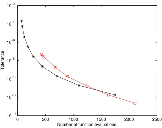
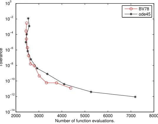
of the Matlab ODE solvers. Indeed, we found that different ways of coding the ODEs might affect the run time with ode45by as much as an order of magnitude! In this paper we further assume that the ODEs are evaluated efficiently for an array of arguments. When coded in this way,BV78solved the problem for a wide range of tolerances in 2.2s andode45did this in 6.1s. Figure 5.2 shows the efficiency in terms of the number of array evaluations. There seem to be too few data points forBV78in this figure. That is because for absolute error tolerances 10−2, . . . ,10−6, the results are all the same—the default maximum step size of one tenth of the length of the interval of integration already provides an error of about 5×10⁻⁸. For testing purposes we provide an option in BV78of integrating with only one argument in each call to evaluate the ODEs. The run time of 10.2s when this is done shows the importance of vectorizing. Nonetheless, Figure 5.3 shows that even without vectorization,BV78is reasonably efficient at all tolerances and at stringent tolerances is comparable to ode45because the higher order compensates for more expensive steps.
6. Conclusions. Our analysis and numerical experiments support the conclusion that if it is convenient to vectorize the function that evaluates the differential equations, BV78 will be comparable to ode45 at all tolerances and considerably more efficient at stringent tolerances. In fact, for a wide range of standard test problems solved for a wide range of tolerances, BV78 required only one third the run time of ode45. This conclusion assumes that the cost of evaluating the vectorized function is not much greater than the cost of evaluating it with a single argument. If that is not the case, BV78 will solve the problem with acceptable efficiency, but it will be slower thanode45at all but stringent tolerances.
Though the scheme we have implemented seems to be a good one, it suggests other possibilities that merit future investigation: The scheme described for evaluating the BV(7,8) pair forms approximate solutions of all local orders from 2 to 8. Clearly it would be possible to develop a variable order code. We have discussed block methods of Newton-Cotes type, but there are other kinds of block methods that might have advantages. For example, a family of implicit block methods with superior stability is studied in [14].
7. Acknowledgement. This paper was improved as a result of valuable comments from W. Enright of the University of Toronto and P. Muir of Saint Mary’s University.
REFERENCES
[1] P. Bogacki and L. F. Shampine,A 3(2) Pair of Runge-Kutta Formulas, Appl. Math. Letters, 2 (1989), pp. 1–9.
0 200 400 600 800 1000 1200 1400 1600 1800 10−14
10−12 10−10 10−8 10−6 10−4 10−2
Number of function evaluations.
Tolerance
Fig. 5.2.C5 is a five body model of the solar system.
0 500 1000 1500 2000 2500 10−14
10−12 10−10 10−8 10−6 10−4 10−2
Number of function evaluations.
Tolerance
Fig. 5.3.C5 when evaluation of the ODEs is notvectorized.
[3] J. R. Dormand,Numerical Methods for Differential Equations a Computational Approach, CRC Press, Boca Raton, FL, 1996.
[4] T. E. Hull, W. H. Enright, B. M. Fellen, and A. E. Sedgwick,Comparing Numerical Methods for Ordinary Differential Equations, SIAM J. Numer. Anal., 9 (1972), pp. 603–637.
[5] J. Kierzenka and L.F. Shampine,A BVP Solver Based on Residual Control and the Matlab PSE, ACM Trans. Math. Softw., 27 (2001), pp. 299–316.
[6] F. T. Krogh,On Testing a Subroutine for the Numerical Integration of Ordinary Differential Equations, J. ACM, 20 (1973), pp. 545–562.
[7] Maple 11, Maplesoft, 615 Kumpf Dr., Waterloo, CA.
[8] W. E. Milne,Numerical Solution of Differential Equations, Dover, Mineola, NY, 1970. [9] J.B. Rosser,A Runge-Kutta for All Seasons, SIAM Rev., 9 (1967), pp. 417–452.
[11] L. F. Shampine and M. W. Reichelt,TheMatlabODE Suite, SIAM J. Sci. Comp., 10 (1997), pp. 1–22. [12] L. F. Shampine and H. A. Watts,Block Implicit One-step Methods, Math. Comp., 23 (1969), pp. 731–740. [13] J. H. Verner, A ’Most Efficient’ Runge-Kutta (13:7,8) Pair, available athttp://www.math.sfu.ca/~jverner/. [14] H. A. Watts and L. F. Shampine,A-Stable Block Implicit One Step Methods, BIT, 12 (1972), pp. 252–256.
Edited by: Pierluigi Amodio and Luigi Brugnano
Received: January 23, 2009
![Table 5.1Run times for test set of Krogh [6].](https://thumb-us.123doks.com/thumbv2/123dok_us/8749990.1748293/6.595.221.408.687.725/table-run-times-test-set-krogh.webp)