Sensitivity Study of Input Parameters for Seepage Flow Simulations using Parallel Computers

(1)

Scalable Computing: Practice and Experience

Volume 17, Number 1, pp. 47–60. http://www.scpe.org

ISSN 1895-1767 c

⃝2016 SCPE

SENSITIVITY STUDY OF INPUT PARAMETERS FOR SEEPAGE FLOW SIMULATIONS USING PARALLEL COMPUTERS∗

FRED T. TRACY†_{, LUCAS A. WALSHIRE}‡_, _AND _{MAUREEN K. CORCORAN}§

Abstract. This paper describes a comprehensive sensitivity study that was performed using high performance parallel com-puters to understand the importance of input parameters to a transient partially saturated finite element seepage analysis for a levee with separate soil layers of sand, silty sand, and clay. Seepage flow in this paper refers to the type of flow of water that occurred through the failed levees in New Orleans, Louisiana, USA, as a result of Hurricane Katrina. The input parameters tested were saturated hydraulic conductivity, volumetric compressibility, residual moisture content, saturated moisture content, and two van Genuchten unsaturated flow parameters. The output data compiled to show the sensitivity of the input parameters were the simulation times (days) to achieve 25%, 50%, and 75% of the steady-state values of pore pressure at the toe of the levee beneath its blanket, flow rate through the landside flux section, and the level of saturation in the levee. The use of high performance parallel computers enabled the running of thousands of scenarios using different values for the input variables. A sensitivity investigation of this magnitude has not been previously performed.

The results of this investigation indicated that the more sensitive soil parameters were the saturated hydraulic conductivity and the volumetric compressibility. The unsaturated van Genuchten parameters of the landside blanket had a larger than anticipated impact on the duration of time to achieve steady state. This practical example is an excellent success story for high performance computing in that running a given simulation for a couple of hours on thousands of processors in parallel replaced over a year’s work using a PC.

Key words: high performance computing, sensitivity analysis, finite element method, seepage flow modeling

AMS subject classifications. 35J66, 65Y05, 76S05

1. Introduction. Historically, the majority of practicing engineers have used two-dimensional (2-D) steady state analyses to design and analyze levees. Finite element programs such as SEEP2D [1,2] in the Groundwater Modeling System (GMS) [3,4] and SEEP/W [5] with excellent graphical user interfaces have greatly aided these design and analysis processes. However, using only steady-state analyses leads to the most conservative and therefore, the most expensive design. With the ability to now do a transient seepage analysis on a computer, key questions are when should a design be based on a transient analysis instead of a steady-state analysis, what soil parameters are important in the transient analysis, and how reliable are the transient simulation results.

One traditional analytical tool used in determining the relative importance of the various input parameters is a sensitivity study. Some sensitivity analyses have been historically too compute-intensive to perform. However, with the availability of high performance, parallel computing, thousands of scenarios can be run at once, allowing for the testing of a greater number of input parameters than was previously possible.

The purpose of this research was to perform a comprehensive sensitivity study of input soil parameters needed for a transient finite element seepage analysis as measured by the response of key output variables. A generic levee common to the southeastern United States was selected for the analysis. To perform the analysis, a parallel program was created such that from a set of data describing the levee cross section, a finite element mesh was generated, initial and boundary conditions were applied, both steady-state and transient seepage analyses were performed, and key data were stored for future analysis. This was all done in the context of parallel computing where thousands of scenarios could be computed simultaneously. A feature of the groundwater modeling program used in the study is that the time needed to achieve a certain percentage of the steady-state value of a given output variable can be computed and stored for future analysis. This is possible because a steady-state solution is computed before the transient solution is performed. This modified parallel groundwater modeling program made this research possible. Because of all the obstacles, very few sensitivity studies of this magnitude have been completed with no known studies performed on this magnitude for transient seepage.

∗_{This work was supported in part by a grant of computer time from the Department of Defense High Performance Computing}

Modernization Program (HPCMP).

†_{Information Technology Laboratory, Engineer Research and Development Center (ERDC), Vicksburg, MS, USA.} ‡_{Geotechnical and Structures Laboratory (GSL), ERDC, Vicksburg, MS, USA.}

§_{GSL, ERDC, Vicksburg, MS, USA.}

(2)

2. Measuring sensitivity. There are many ways to measure sensitivity of an output variable to an input parameter, and an excellent description of them is given in [6]. This information will not be repeated here but rather some key methods of doing sensitivity studies for numerically intensive applications are highlighted. The method of slopes and the method of ranges were used in this investigation.

2.1. Method of slopes. Changing only one input parameter while holding all the others constant and measuring the output to obtain the slope of the output variable versus the varied input parameter curve is the simplest way of doing a sensitivity analysis [6]. The slope, m, for a given output value (Y) versus input parameter (X) curve is simply the partial derivative,

m= ∂Y

∂X (2.1)

This curve can be determined by using different values ofX, running the transient seepage program, and then recording the resultingY output values. Because this slope was determined numerically, it was approximated as follows:

m≈ ∆Y

∆X (2.2)

where ∆X is a small increment of input parameter, and ∆Y is the resulting small change in the output value. Only one type of output parameter was considered in this study, but several input parameters varying over several orders of magnitude were considered. Therefore, a sensitivity coefficient, sm, fashioned after [7] was implemented. DefiningY(X) as the output,Y, as a function of the input parameter,X,smis

sm= Y(

X+100p X )

−Y(X)

p (2.3)

where p is a percentage of a given input parameter. Because of the highly nonlinear nature of the governing partial differential equation where repeated Picard or Newton iterations [8] are needed, a value ofp= 10 was selected. The sensitivity coefficient,sm, can be computed for different values of the input parameters to obtain an overall view of the nonlinear behavior.

2.2. Method of ranges. The method of ranges is useful when the output can be sampled over the entire range of the respective input parameters. This method compares how much the output variable changes when the different input parameters are varied. A sensitivity coefficient based on ranges is now defined, which is an extension of previous work [9]. The case where there are i = 1,2,3, . . . , M scenarios of thej = 1,2,3, . . . , N input parameters was considered. DefiningKj as the number of different values of thejthinput parameter,M in this research becomes

M =K1K2K3· · ·KN = N ∏

j=1

Kj (2.4)

Eq. 2.4 is rearranged to isolate the jth_{input parameter as follows:}

M =



 N ∏

i=1,i̸=j Ki



Kj=MjKj (2.5)

where Mj is the number of combinations of all the input parameters except the jth one. For each of these m = 1,2,3, . . . , Mj combinations, the results of varying thejth input parameter over its range while holding the other input parameters constant are used to define a sensitivity coefficient based on the range of the output values. The sensitivity coefficient for this mth _{scenario while changing only the}_jth _{input parameter is defined} as follows:

sj_rm= (Ymax)mj−(Ymin)mj Ymax−Ymin

(3)

where

(Ymin)_mj = minimum value of output, Y, when varying the jth _{input parameter and holding the others} constant for themth combination

(Ymax)_mj = maximum value of output, Y, when varying the jth _{input parameter and holding the others} constant for themth _combination

Ymin = overall minimum value of the output variable,Y Ymax = overall maximum value of the output variable,Y

The overall sensitivity coefficient for thejth_{input parameter is computed by taking the maximum value of the} sj

rm values over theMj combinations. That is, sj

r= Mj

max m=1 (

sj rm

)

(2.7)

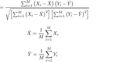
2.3. Statistical methods. There are many statistical methods for calculating sensitivity. One of the simplest methods that uses simple correlation coefficients was derived from Monte Carlo simulations [10]. Here, Pearson’s product moment correlation coefficient [11] was employed. The case that is now considered is where M output values are computed fromM values of an input parameter,X. Pearson’s product moment correlation coefficient is given by

r=

∑M i=1

( Xi−X¯

) ( Yi−Y¯

)

√ [

∑M i=1

( Xi−X¯

)2] [∑M i=1

( Yi−Y¯

)2]

(2.8)

¯ X = 1

M M ∑

i=1

Xi (2.9)

¯ Y = 1

M M ∑

i=1

Yi (2.10)

The larger the r value, the stronger the reaction of the output to the input [12]. This works best when the relationship between input parameter and output variable is linear. However, the application presented in this paper is highly nonlinear.

3. Levee. Eqs. 2.3 and 2.7 were applied to a generic levee. The geometry, material properties, initial conditions, boundary conditions, and hydrograph of the river are provided in the following subsections. Detail is provided for those practicing geotechnical engineers who find such information important.

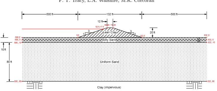
3.1. Generic levee cross section. A 2-D finite element model of a generic levee cross section represen-tative of the southeastern United States is shown in Fig. 3.1 (this section is further described in [13]). This model was used to perform computations and to do the sensitivity study described in this paper.

3.2. Riverside and landside water elevation. The initial river elevation was set to -5 ft. An initial water elevation below the ground surface is the most interesting case because the water must rise through two of the three soil layers as it reaches its maximum height. The river elevation advanced at 2 ft/day until it reached 17.5 ft where it was held constant indefinitely. This is illustrated in the hydrograph shown in Fig. 3.2 where the time for the hydrograph is plotted for only 30 days but extends indefinitely.

(4)

Fig. 3.1: Generic levee cross section showing three separate layers of sand, silty sand, and clay.

Fig. 3.2: Hydrograph that starts at -5 ft and then goes up 2 ft/day until 17.5 ft is reached and then remains constant indefinitely.

Table 4.1: Parameters used in the levee system study.

Name Symbol

Saturated hydraulic conductivity (ft/day) k_s Residual volumetric water content (unitless) θ_r Saturated volumetric water content (unitless) θs

First van Genuchten parameter (1/ft) α Second van Genuchten parameter (unitless) n Volumetric compressibility(1/psf) m_v

5. Output variables selected for the sensitivity study. The output variables selected for this research are the simulation time in days to achieve 25%, 50%, and 75% of the steady-state values of the following three quantities:

• The pore pressure (psf) at the toe of the levee beneath the blanket (coordinates 132, -10 in Fig. 3.1). • The flow rate per unit length (ft3/day/ft) of water leaving the flux section, (132, 0) to (632, 0) to (632,

-90) in Fig. 3.1.

• Levee saturation coefficient.

The levee saturation coefficient is defined as

SL = ∫ ∫

Aθ(x, y, t)dxdy− ∫ ∫

Aθ(x, y,0)dxdy ∫ ∫

Aθ(x, y,∞)dxdy− ∫ ∫

Aθ(x, y,0)dxdy

(5)

Table 6.1: Values of input parameters used in the homogeneous case.

Parameter Value

θ_r _0.034

θs 0.46

α _{0.488 ft}−1

n 1.37

m_v 1.0×10−5psf−1

where

A = area of the levee

θ(x, y, t) = volumetric moisture content of an (x, y) point in the levee at time,t θ(x, y,0) = volumetric moisture content of an (x, y) point in the levee att= 0

θ(x, y,∞) = volumetric moisture content of an (x, y) point in the levee at steady state

It is important to note that 0≤SL≤1 sinceSL= 0 at initial conditions, andSL= 1 at steady state.

6. Homogeneous case. In the first case, the aquifer, confining blanket, and levee materials were assigned identical soil properties.

6.1. Varying only the saturated hydraulic conductivity. The approach used in this research was to start with the simplest case and build on that effort with more complicated scenarios. In this initial run, only saturated hydraulic conductivity was varied with values, 0.001, 0.01, 0.1, 1.0, 10.0, and 100.0 ft/day (3.528×10−7

, 3.528×10−6

, 3.528×10−5

, 3.528×10−4

, 3.528×10−3

, and 3.528×10−2

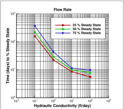
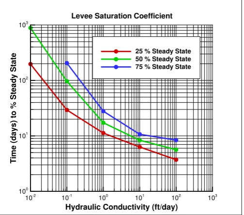
cm/sec, respectively). The hydraulic conductivity values correspond to the following material types: clay, silt, silty sand, fine sand, and coarse sand, respectively [14]. Table 6.1 gives the values of the other input parameters used for these runs. Figs. 6.1, 6.2, and 6.3 show the times to achieve 25, 50, and 75% of the respective steady-state values of the pore pressure at the toe of the levee beneath the blanket, the flow rate through the flux section, and the levee saturation coefficient, respectively. The computer runs were terminated after 1000 days, so in the cases where more than 1000 days are needed to achieve the given percentages of steady state, no values are plotted. Observations are as follows:

• The saturated hydraulic conductivity has a significant impact on results.

• For hydraulic conductivity values of 0.001 ft/day and 0.01 ft/day, none of the given percentages of the steady-state values of the pore pressure beneath the blanket at the toe and the flow rate through the flux section can develop within 1000 days.

• The same basic trend occurs in each plot with only the separation among curves varying.

6.2. Varying the saturated hydraulic conductivity and volumetric compressibility. Once it was found that the magnitude of the hydraulic conductivity value had a significant impact on the results of a transient analysis, other parameters were varied in conjunction with the hydraulic conductivity. Here, bothks andmv were varied and results collected for the same times to percentage of steady state as before. mv values of 1.0×10−3

, 1.0×10−5

, and 1.0×10−7

psf−1 were used with the sameks values as before. The results are given in Figs. 6.4, 6.5, and 6.6. It is important to note that all combinations of ks and mv are not what a practicing engineer may choose. However, to maintain continuity of trends, they are kept in the plots. The method of ranges (Eq. 2.7) was applied to these results, and the result of this computation is provided in Table 6.2. For all computations in this paper where Eq. 2.7 is used, Ymax = 1000. Observations from these results are:

• mv has a significant impact on results but slightly less influence thanks.

(6)

Hydraulic Conductivity (ft/day)

T

im

e

(d

a

y

s

)

to

%

S

te

a

d

y

S

ta

te

10-2

10-1

100

101

102

103

100

101

102

103

25 % Steady State 50 % Steady State 75 % Steady State

Pore Pressure

Fig. 6.1: Plot of times to percentage of steady state for pore pressure.

T

im

e

(d

a

y

s

)

to

%

S

te

a

d

y

S

ta

te

10-2

10-1

100

101

102

103

100

101

102

103

Flow Rate

Fig. 6.2: Plot of times to percentage of steady state for flow rate through the flux section.

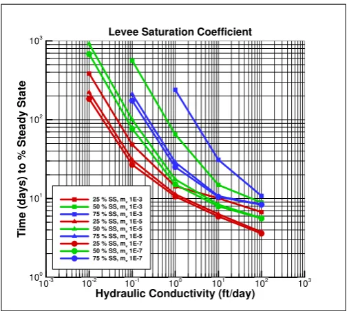
6.3. Varying all input parameters except volumetric compressibility. The next analysis was per-formed with all input parameters being varied except mv, andsr was computed as before using Eq. 2.7. The values of the parameters used in this analysis are given in Table 6.3. There are two reasons why only mv = 0.00001 psf−1 was used, and they are as follows: (1) Whenmv was set to 0.001, 0.00001, and 0.0000001 psf−

1

as before, all thesrvalues were 0.99. Thus, no separation of importance was possible. (2)mv = 0.00001 psf− 1

(7)

T

im

e

(d

a

y

s

)

to

%

S

te

a

d

y

S

ta

te

10-2

10-1

100

101

102

103

100

101

102

103

Levee Saturation Coefficient

Fig. 6.3: Plot of times to percentage of steady state for levee saturation coefficient.

T

im

e

(d

a

y

s

)

to

%

S

te

a

d

y

S

ta

te

10-3

10-2

10-1

100

101

102

103

100

101

102

103

25 % SS, mv1E-3 50 % SS, mv1E-3 75 % SS, mv1E-3 25 % SS, mv1E-5 50 % SS, mv1E-5 75 % SS, mv1E-5 25 % SS, mv1E-7 50 % SS, mv1E-7 75 % SS, mv1E-7

Pore Pressure

Fig. 6.4: Plot of times to percentage of steady state for pore pressure for ks andmv combinations.

• The saturated hydraulic conductivity was shown to be the most sensitive input variable. • The other input parameters ofθr,θs,α, and nall have significant influence on results. • αandnare the most sensitive of the unsaturated flow parameters.

(8)

T

im

e

(d

a

y

s

)

to

%

S

te

a

d

y

S

ta

te

10-3

10-2

10-1

100

101

102

103

100

101

102

103

Flow Rate

Fig. 6.5: Plot of times to percentage of steady state for flow rate through the flux section for ks and mv combinations.

T

im

e

(d

a

y

s

)

to

%

S

te

a

d

y

S

ta

te

10-3

10-2

10-1

100

101

102

103

100

101

102

103

Levee Saturation Coefficient

Fig. 6.6: Plot of times to percentage of steady state for levee saturation coefficient forksandmv combinations.

the variation of soil types in the three layers, and Table 7.2 gives the values of soil properties used. The 14 allowable combinations of saturated hydraulic conductivity for the levee and blanket are given in Table 7.3. Saturated hydraulic conductivity values considered for the aquifer areks,aquif er = 10 and 100 ft/day.

(9)

Table 6.2: Sensitivity coefficient, sr, values for ks andmv for the times to different percentages of steady state for pore pressure, flow rate, and levee saturation coefficient.

srfor pore pressure

Percent of steady state Input parameter 25 50 75

k_s 0.9973 0.9967 0.9950 m_v _0.9696 _0.9415 _0.9148

s_rfor flow rate

k_s _0.9945 _0.9922 _0.9901 mv 0.9065 0.8605 0.9686

s_r _{for levee saturation coefficient} Percent of steady state Input parameter 25 50 75

ks 0.9964 0.9944 0.9916

m_v 0.2010 0.4863 0.8255

Table 6.3: Range of input parameters.

Material Property Range of Values Investigated ks(ft/day) 0.001, 0.01, 0.1, 1, 10, 100

m_v(1/psf) 1.0×10−5

θ_r _{0.05, 0.1, 0.15} θ_s _{0.40, 0.45, 0.5} α(1/ft) 0.2, 0.4, 0.6

n 1.25, 1.75, 2.25

Table 6.4: Sensitivity coefficient, sr, values for ks, θr, θs, α, and n for the times to different percentages of steady state for pore pressure, flow rate, and levee saturation coefficient.

srfor pore pressure

k_s _0.9969 _0.9969 _0.9951 θ_r _0.1459 _0.1486 _0.1287 θ_s _0.1459 _0.1486 _0.1287 α 0.3154 0.3048 0.2591 n 0.4503 0.4046 0.3186

srfor flow rate

k_s 0.9945 0.9922 0.9901 θ_r _0.0961 _0.0672 _0.1146 θ_s _0.0961 _0.0672 _0.1146 α 0.1874 0.1637 0.3257 n 0.1874 0.1767 0.3072 sr for levee saturation coefficient

(10)

Table 7.1: Description of soils in levee layers.

Layer Material variation Levee Clay to gravelly sand Blanket Clay to sandy silt Aquifer Sand to gravelly sand

Table 7.2: Soil property data for selected soils.

Soil classification k_s _(ft/day) θ_r θ_s α_(1/ft) n m_v_(1/psf) Clay 0.001 0.05 0.50 0.076, 0.137 1.05 5×10−5

Lean clay 0.01 0.045 0.45 0.152, 0.228 1.1, 1.15 1×10−5

Silt 0.1 0.04 0.40 0.243, 0.610 1.2, 1.35 5×10−6

Silty sand/sandy silt 1 0.035 0.35 0.762, 1.829 1.4, 1.6 1×10−6

Sand 10 0.03 0.30 2.286, 4.420 1.9, 2.7 5×10−7

Gravelly sand 100 Not used 1×10−7

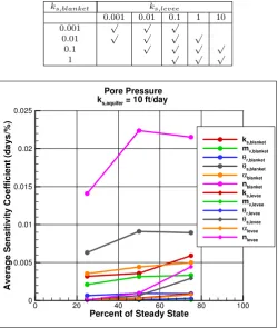
Table 7.3: Hydraulic conductivity (ft/day) combinations for levee, blanket, and aquifer layers. The check marks indicate the allowable combinations.

k_s,blanket k_s,levee

0.001 0.01 0.1 1 10

0.001 √ √ √

0.01 √ √ √ √

0.1 √ √ √ √

1 √ √ √

Percent of Steady State

A

v

e

ra

g

e

S

e

n

s

it

iv

it

y

C

o

e

ff

ic

ie

n

t

(d

a

y

s

/%

)

0 20 40 60 80 100

0 0.005 0.01 0.015 0.02 0.025

ks,blanket

mv,blanket θ

r,blanket θ

s,blanket α

blanket

nblanket

ks,levee

mv,levee θ

r,levee θ

s,levee α

levee

nlevee Pore Pressure

k_s,aquifer= 10 ft/day

Fig. 7.1: Plot of averagesm for pore pressure forks,aquif er = 10 ft/day.

(11)

Percent of Steady State A v e ra g e S e n s it iv it y C o e ff ic ie n t (d a y s /% )

0 20 40 60 80 100

0 0.002 0.004 0.006 0.008 ks,blanket mv,blanket θ r,blanket θ s,blanket α blanket nblanket ks,levee mv,levee θ r,levee θ s,levee α levee nlevee Pore Pressure

Fig. 7.2: Plot of averagesmfor pore pressure forks,aquif er = 100 ft/day.

A v e ra g e S e n s it iv it y C o e ff ic ie n t (d a y s /% )

0 20 40 60 80 100

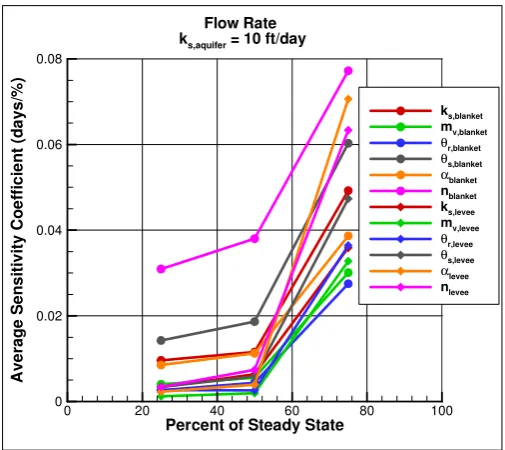
0 0.02 0.04 0.06 0.08 ks,blanket mv,blanket θ r,blanket θ s,blanket α blanket nblanket ks,levee mv,levee θ r,levee θ s,levee α levee nlevee Flow Rate

Fig. 7.3: Plot of averagesm for flow rate forks,aquif er = 10 ft/day.

(12)

Percent of Steady State A v e ra g e S e n s it iv it y C o e ff ic ie n t (d a y s /% )

0 20 40 60 80 100

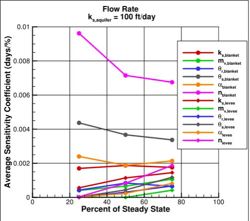
0 0.002 0.004 0.006 0.008 0.01 ks,blanket mv,blanket θ r,blanket θ s,blanket α blanket nblanket ks,levee mv,levee θ r,levee θ s,levee α levee nlevee Flow Rate

Fig. 7.4: Plot of averagesmfor flow rate forks,aquif er = 100 ft/day.

A v e ra g e S e n s it iv it y C o e ff ic ie n t (d a y s /% )

0 20 40 60 80 100

0 1 2 3 4 ks,blanket mv,blanket θ r,blanket θ s,blanket α blanket nblanket ks,levee mv,levee θ r,levee θ s,levee α levee nlevee Levee Saturation Coefficient

Fig. 7.5: Plot of averagesm for levee saturation coefficient forks,aquif er = 10 ft/day.

with ks,aquif er = 10 ft/day, and another withks,aquif er = 100 ft/day. Thus, two sets of 2444 simulations each were needed. All 2444 simulations for a givenks,aquif er value were accomplished with a parallel MPI job using 2444 processes and taking approximately 1.5 hours.

(13)

A

v

e

ra

g

e

S

e

n

s

it

iv

it

y

C

o

e

ff

ic

ie

n

t

(d

a

y

s

/%

)

0 20 40 60 80 100

0 1 2 3 4 5

ks,blanket

mv,blanket θ

r,blanket θ

s,blanket α

blanket

nblanket

ks,levee

mv,levee θ

r,levee θ

s,levee α

levee

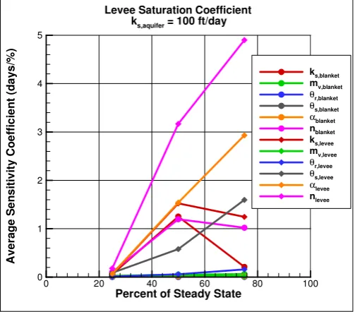
nlevee Levee Saturation Coefficient

Fig. 7.6: Plot of averagesmfor levee saturation coefficient forks,aquif er = 100 ft/day.

and the average value ofsm over these valid combinations for each input parameter was tabulated. Both runs for ks,aquif er = 10 and 100 ft/day were done, and the results are given in Figs. 7.1, 7.2, 7.3, 7.4, 7.5, and 7.6. Observations are as follows:

• Pore pressure at the toe of the levee and flow rate are 2-3 orders of magnitude less sensitive to the input parameters than is the levee saturation coefficient.

• The input parameters for both the blanket and the levee are important.

• The second van Genuchten unsaturated flow parameter,n, is the most sensitive input variable for most of the scenarios analyzed.

• The sensitivity coefficients for pore pressure and flow rate are approximately an order of magnitude less whenks,aquif er = 100 ft/day as compared toks,aquif er = 10 ft/day.

8. Conclusions. This sensitivity study considered a large number of scenarios and was made feasible only through the use of high performance, parallel computers. This is especially true because the scenarios can be run independently without any communication among MPI processes. The results of the study indicate the need to obtain all the input parameters (saturated hydraulic conductivity, volumetric compressibility, residual moisture content, saturated moisture content, and the two van Genuchten parameters) as accurately as possible since the output quantities of interest show a significant sensitivity to each parameter for at least some of the scenarios analyzed. The volumetric compressibility had a dominant effect on output values in the homogeneous case but ranked near the bottom of the list in the case where all three layers had different material properties. The second van Genuchten parameter ranked low in sensitivity in the homogeneous case for pore pressure and flow rate but ranked very high when all three layers had different material properties. When all three layers had different material properties, the van Genuchten unsaturated flow parameters for the blanket often dominated for pore pressure and flow rate, whereas the unsaturated flow parameters for the levee dominated for levee saturation coefficient.

(14)

a local value that varies greatly over the different scenarios. A simple average of the results over the different scenarios as presented here could be improved with a more sophisticated analysis. This is a topic of future research.

The method of ranges is acceptable for the application presented in this paper, but it has the disadvantage that many scenarios are needed to explore a full range of input parameters and thus to obtain comprehensive results. However, the number of combinations of input parameters can be reduced by limiting the scenarios to only those of interest to practicing engineers.

REFERENCES

[1] F. T. Tracy,User’s guide for a plane and axisymmetric finite element program for steady state seepage problems, Instruction

Report IR K-83-4, U.S. Army Engineer Research and Development Center, Vicksburg, MS, 1983.

[2] N. L. Jones,SEEP2D primer, GMS documentation, Environmental Modeling Research Laboratory, Brigham Young

Univer-sity, Provo, Utah, 1999.

[3] GMS,Groundwater Modeling System, commercial version, www.aquaveo.com/GMS, 2016.

[4] GMS,Groundwater Modeling System, government version, http://chl.erdc.usace.army.mil/gms, 2016.

[5] Geo-Slope,Seepage modeling with SEEP/W, Calgary, Alberta, Canada, 2012.

[6] D. M. Hamby,A review of techniques for parameter sensitivity analysis of environmental models, Environmental Monitoring

and Assessment, 32 (1994), pp. 135-154.

[7] R. W. Atherton, R. B. Schainker, and E. R. Ducot,On the statistical sensitivity analysis of models for chemical kinetics,

AIChE, 21 (1975), pp. 441-448.

[8] S. Mehl,Use of Picard and Newton iteration for solving nonlinear ground water flow equations, Ground Water, 44 (2006),

pp. 583-594.

[9] F. O. Hoffman and R. H. Gardner,Evaluation of uncertainties in environmental radiological assessment models, In: J. E.

Till and H. R. Meyer (eds.), Radiological Assessments: a Textbook on Environmental Dose Assessment, Report No. NUREG/CR-3332, U.S. Nuclear Regulatory Commission, Washington, DC, 1983.

[10] R. H. Gardner, R. V. O’Neill, J. B. Mankin, and J. H. Carney,A comparison of sensitivity analysis and error analysis

based on a stream ecosystem model, Ecol. Modelling, 12 (1981), pp. 173-190.

[11] W. J. Conover,Practical Nonparametric Statistics, 2nd edition, Oxford University Press, John Wiley & Sons, New York,

1980.

[12] International Atomic Energy Agency (IAEA),Evaluating the reliability of predictions made using environmental transfer

models, Safety Series No. 100, Report No. STI/PUB/835, Vienna, Austria, pp. 1-106, 1989.

[13] F. T. Tracy, T. L. Brandon, and M. K. Corcoran,Transient seepage analyses in levee engineering practice, In review,

U.S. Army Engineer Research and Development Center, Vicksburg, MS, 2016.

[14] K. Terzaghi, B. Peck, and G. Mesr,Soil Mechanics in Engineering Practice, John Wiley & Sons, New York, 1996.

Edited by: Dana Petcu

Received: Dec 18, 2015