Organized by C.O.E.T, Akola. Available Online at www.ijpret.com
386
INTERNATIONAL JOURNAL OF PURE AND
APPLIED RESEARCH IN ENGINEERING AND
TECHNOLOGY
A PATH FOR HORIZING YOUR INNOVATIVE WORK
APPLICATION OF SOFT COMPUTING TECHNIQUE TO SIMULATE YIELD OF
IRRIGATED TOMATO
KALE M.U.
1, WADATKAR S.B.
21.Assistant professor, Deptt. of Irrigation and Drainage Engineering, Dr. Panjabrao Deshmukh Krishi Vidyapeeth, Akola, (MS) India. 2.Head of Deptt., Deptt. of Irrigation and Drainage Engineering, Dr. Panjabrao Deshmukh Krishi Vidyapeeth, Akola, (MS) India
Accepted Date: 05/09/2017; Published Date: 10/10/2017
Abstract:
Field verification of AquaCrop model results for irrigated tomato was carried out to test the AquaCrop model as a soft computing tool to improve water use efficiency. AquaCrop model was calibrated using tomato production data for the year 2013-2015. The calibrated value of harvest index and water productivity was 65% and 35 gm-2, respectively. Simulations were carried out with formulated schedules for the period 17th October 2014 to 1sh March2015. AquaCrop predicted schedule S3 (mulch + Irrigation schedule at 75 % ETc) as the best schedule based on maximum water use efficiency i.e. 12.84 qha-cm -1. This schedule S
3 (treatment T6) was tested in the field during 2015-16 along with other treatments. The maximum yield is recorded in treatment T3 (mulch +
Irrigation schedule at 80 % ETc) i.e. 263.66 qha-1 followed by T6 (mulch + Irrigation schedule at 75 % ETc) i.e. 262.05 qha-1. But water use efficiency was found
maximum for T6 (12.73 qha-cm-1) followed by T3 as (12.12 qha-cm-1). Therefore it is recommended to implement T6 i.e. silver mulch + Irrigation schedule at 75
% ETc, for tomato production in western Vidarbha region. The results also confirmed the capability of AquaCrop in predicting the effect of water on the yield of
tomato.
Keywords
: Crop water productivity, Water use efficiency, AquaCrop, tomato, crop evapotranspiration.
Corresponding Author: KALE M.U.
Co Author: - WADATKAR S.B.
Access Online On:
www.ijpret.com
How to Cite This Article:
Kale M. U., IJPRET, 2017; Volume 6 (2): 386-393
PAPER-QR CODE
SPECIAL ISSUE FOR
INTERNATIONAL LEVEL CONFERENCE
"ADVANCES IN SCIENCE,
Organized by C.O.E.T, Akola. Available Online at www.ijpret.com
387
INTRODUCTION
Agriculture, being the major water user, its share in the total freshwater demand is bound to decrease from the present 83% to 68% due to more pressing and competing demands from other sectors by 2050 AD (GOI, 2013). There is a need to increase annual foodgrain production from about 210 million tonnes (2013) to 420 million tonnes by 2015. Since water is a shrinking resource for agriculture, the pathway for achieving this goal has to be higher productivity per unit of water. Thus, the objective of agricultural production in the present era is not only to provide supplementary water for crop production but also to decrease crop water use per unit yield of crop i.e.
more crop per drop (Swaminathan, 2013).
Tomato is a popular and nutritive vegetable crop ranking next to potato in world’s vegetable production. Tomato is an important source of minerals and antioxidants, which have a key role in human nutrition to prevent certain cancer and cardio vascular diseases. In 2014-15, in India total area under tomato cultivation was 882 thousand ha,
total production was 18735.9 thousand MT and total productivity was 21.2 MTha-1. While, in Maharashtra state
total area under tomato was 50 thousand ha, total production was 1200 thousand MT and total productivity was
24 MTha-1 (NHB, 2014).
Accurate crop development models are important tools in evaluating the effects of water deficits on crop yield or productivity. AquaCrop is developed from revision of ‘FAO Irrigation and Drainage Paper No. 33 Yield Response to Water’ (Doorenbos et al., 1979). It simulates crop yield in response to water, and is particularly suited to address conditions where water is a key limiting factor in crop production. The potential of AquaCrop model in simulating the yield in response to water is proved by various researchers (Araya et al. 2010a, Heng et al. 2009; Stricevic et al. 2011; Abedinpour et al. 2012, Andarzian et al. 2011).
Tomato has the highest acreage of any vegetable crop in the world, therefore adoption of deficit irrigation could make substantial contribution to saving of water. Thus, considering the need of enhancing water use efficiency, this research study was undertaken.
2. MATERIAL AND METHODS
2.1. Data collection
Meteorological data for the period 23rd October 2013 to 28th February 2016 was obtained from
Agro-meteorological Observatory, Dr. P.D.K.V., Akola.
The required crop data was obtained from a field experiment conducted during the year 2013 - 2015 and having following treatments.
Sr. No. Treatment Specification
1 T1 40 % ETc with silver polyethylene mulch
2 T2 60 % ETc with silver polyethylene mulch
3 T3 80 % ETc with silver polyethylene mulch
4 T4 100 % ETc with silver polyethylene mulch
5 T5 100 % ETc without polyethylene mulch (control)
Organized by C.O.E.T, Akola. Available Online at www.ijpret.com
388
2.2. Background of AquaCrop model
FAO Irrigation and Drainage Paper No. 33 (Doorenbos et al., 1979) represented an important source to determine the crop yield response to water through the following equation:
a a
y
x x
Y
ET
1-
= k
1-Y
ET
….. (1)where,
x
Y
andY
a - Maximum and actual yield,x
ET
andET
a - Maximum and actual evapotranspiration, andy
k
- Crop yield factor2.3. Calibration and validation of model
The data of field experiment conducted during the period 2014-15 and 2013-14, was used for calibration and validation of the model, respectively. The model was calibrated by varying harvest index and water productivity. AquaCrop version 4.0 was used in the study.
2.4. Model performance
Statistical parameters viz. Nash Sutcliffe coefficient (Nash and Sutcliffe, 1970) and coefficient of residual mass (Kale, 2014) were used to judge the performance of the model.
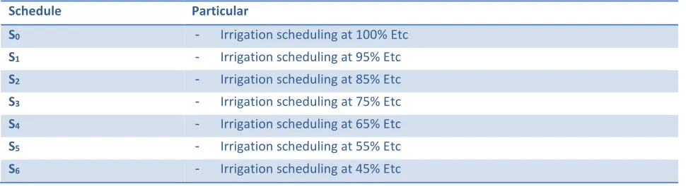
2.5. Formulation of irrigation schedules
Crop evapotranspiration (ETc) was computed on daily basis using values of crop coefficients (Holsambare,1988) and reference evapotranspiration (Allen et al., 1998). Seven schedules were formulated considering various levels of water application i.e. ETc as follows.
Table 2 Formulated irrigation schedules
Schedule Particular
S0 - Irrigation scheduling at 100% Etc
S1 - Irrigation scheduling at 95% Etc
S2 - Irrigation scheduling at 85% Etc
S3 - Irrigation scheduling at 75% Etc
S4 - Irrigation scheduling at 65% Etc
S5 - Irrigation scheduling at 55% Etc
S6 - Irrigation scheduling at 45% Etc
2.6. Effectiveness of formulated schedules
Organized by C.O.E.T, Akola. Available Online at www.ijpret.com
389
3Total tomato yield, kg
WUE =
Total water applied, m
…..(2)2.7 Field evaluation of best schedule
The best schedule predicted by AquaCrop model was evaluated in the field along with all previous treatments of the field experiment of which data used to calibrate the AquaCrop model. Thus the experiment now consists of six treatments having four replications as below.
Table 3 Treatment details of field experiment
Sr. No. Treatment Irrigation schedule
1 T1 40% ETc with silver polyethylene mulch
2 T2 60% ETc with silver polyethylene mulch
3 T3 80% ETc with silver polyethylene mulch
4 T4 100% ETc with silver polyethylene mulch
5 T5 100% ETc without polyethylene mulch
6 T6 Best schedule predicted by AquaCrop model
In order to observe growth and yield of tomato as affected by different irrigation mulch treatments, biometric observation such as plant height, number of branches and leaf area index were observed at 30, 60, 90 and 120 days after transplanting. Polar and equator diameter of tomato, weight of tomato and yield were observed at the time of harvesting. The best treatment was optimized based on WUE.
3. RESULTS AND DISCUSSION
3.1 Calibration of AquaCrop model
The variation of observed and simulated yield during calibration is depicted in Fig. 1.
10 13 16 19 22
T1 T2 T3 T4
Y
ie
ld,
t ha
-1
Treatments
Observed Yield
Simulated Yield
0 4 8 12 16 20
0 5 10 15 20
S
imul
a
ted
y
ie
ld,
t ha
-1
Observed yield, t ha-1
2014-15
R2
NS = 0.95 CRM = -0.0336
Fig. 1 Comparison between observed and simulated yield over calibration period
The observed yield varied between10.86 to18.63 tha-1, whereas simulated yield varied between 11.63 to 18.30 tha
-1. Observed and simulated yield were in close match, as seen in Fig. 1. Simulated yield of tomato was observed to
Organized by C.O.E.T, Akola. Available Online at www.ijpret.com
390
model slightly overestimated the yield for all treatment except treatment T3. The slightly overestimation of yield by model is supported by coefficient of residual mass as -0.0336. The average variation between observed and simulated yield was found to be 3.92%. It was also supported by good estimate of statistical parameters i.e. Nash Sutcliffe coefficient as 0.95 and CRM as -0.0336. As such the model setup was considered as calibrated and calibrated model parameters are presented in Table 4.
Table 4 Calibrated model parameters
Particulars Measure
Harvesting index, % 65
Water productivity (WP), gm-2 35
3.2 Validation of AquaCrop model
Model validation is in fact the extension of calibration process. Thus model was validated for the period 23rd
October 2013 to 3rd March 2014. The variation in observed and simulated yield of tomato for validation period is
depicted in Fig. 2.
5 8 11 14 17
T1 T2 T3 T4
Y
ie
ld,
t ha
-1
Treatments
Observed
Simulated
0 4 8 12 16 20
0 5 10 15 20
S
imul
a
ted
y
ie
ld,
t ha
-1
Observed yield, t ha-1
2013-14
R2
NS = 0.96 CRM = -0.031
Fig. 2 Comparison between observed and simulated yield for validation period
Likewise calibration, observed and simulated yield were in close match for validation period. Similar to calibration, the model slightly overestimated the yield for all treatment. Considering overall acceptability of results in terms of statistical parameters (Nash Sutcliffe coefficient as 0.96 and CRM as -0.031), the model was considered as validated.
3.3 Response of tomato to various formulated schedules
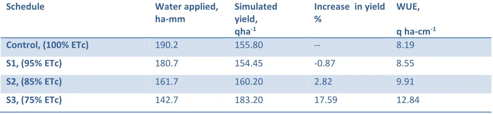
Water use efficiency (WUE) for different formulated irrigation schedules was estimated and presented in Table 5.
Table 5 Water use efficiency for different formulated schedules
Schedule Water applied,
ha-mm
Simulated yield, qha-1
Increase in yield %
WUE,
q ha-cm-1
Control, (100% ETc) 190.2 155.80 -- 8.19
S1, (95% ETc) 180.7 154.45 -0.87 8.55
S2, (85% ETc) 161.7 160.20 2.82 9.91
Organized by C.O.E.T, Akola. Available Online at www.ijpret.com
391
S4, (65% ETc) 123.6 132.35 -15.05 10.71
S5, (55% ETc) 104.2 127.64 -18.07 12.25
S6, (45% ETc) 85.6 122.76 -21.21 14.34
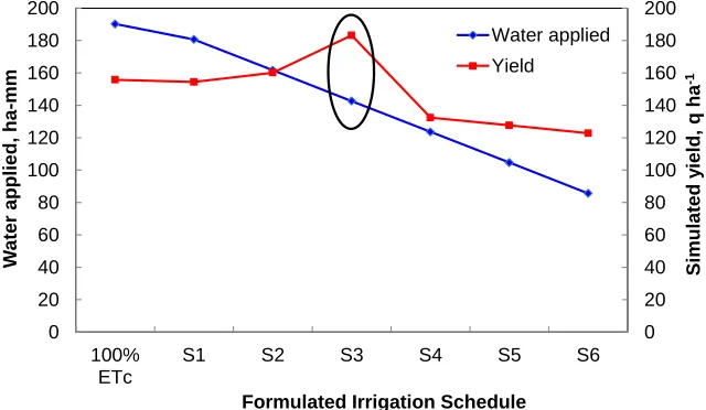
Water applied varied from 85.6 to 190.2 ha-mm. The simulated yield varied from 122.76 to 183.20 qha-1. The
variation in simulated yield ranged from -21.21 to 17.59 qha-1 compared to control treatment. Fig. 3 depicts
variation in simulated yield with reference to water applied.
0 20 40 60 80 100 120 140 160 180 200
0 20 40 60 80 100 120 140 160 180 200
100% ETc
S1 S2 S3 S4 S5 S6
Si
mulated
y
ie
ld,
q ha
-1
W
a
ter
a
pplie
d,
ha
-mm
Formulated Irrigation Schedule
Water applied
Yield
Fig. 3 Variation in simulated yield with reference to water applied
The WUE varied from 8.19 to 14.34 qha-cm-1. The WUE increases as water applied decreases except for schedule
S3. In case of schedule S3, WUE increases though water applied decreased. It was due to increased simulated yield.
The WUE for schedule S3 is estimated as 12.84 qha-cm-1 and is highest among all formulated schedule except
schedule S6. In case of schedule S6, WUE increased due to lowest water applied and lowest simulated yield. Therefore the schedule S3 was emerged as the best formulated schedule.
3.4 Field verification of best schedule predicted by AquaCrop model
3.4.1 Irrigation requirement of tomato
Irrigation water applied during different growth stages of tomato was estimated and presented in Table 6.
Table 6 Crop growth stage wise water requirement Sr.
No.
Crop stage Water applied per plant, lit
T1 T2 T3 T4 T5 T6
1 Common irrigation
before transplanting
13.50 13.50 13.50 13.50 13.50 13.50
2 Initial stage 3.22 4.84 6.45 8.06 8.06 6.05
3 Crop development 13.30 19.95 26.60 33.25 33.25 24.94
4 Mid season 18.14 27.21 36.28 45.35 45.35 34.01
5 Late season 7.54 11.30 15.07 18.84 18.84 14.13
Organized by C.O.E.T, Akola. Available Online at www.ijpret.com
392
ha-cm 12.38 17.07 21.76 26.44 26.44 20.58
(*No rainfall received during the crop season)
The amount of water applied varied from 12.38 to 26.44 ha-cm. It was found maximum for treatment T4 and T5, while minimum for treatment T1. It is observed that maximum water was required by tomato during mid season stage followed by crop development stage, late season, and initial stage, irrespective of treatment.
3.4.2 Water use efficiency
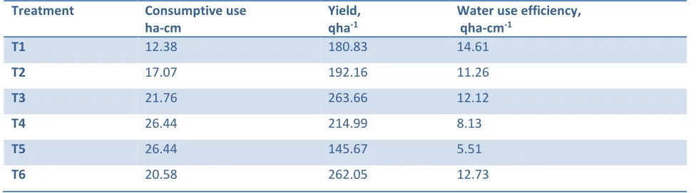
Tomato yield and estimated water use efficiency as influenced by different irrigation/mulch treatments are presented in Table 7.
Table 7 Tomato yield and water use efficiency
Treatment Consumptive use
ha-cm
Yield, qha-1
Water use efficiency, qha-cm-1
T1 12.38 180.83 14.61
T2 17.07 192.16 11.26
T3 21.76 263.66 12.12
T4 26.44 214.99 8.13
T5 26.44 145.67 5.51
T6 20.58 262.05 12.73
In field experiment WUE was found varying between 5.51 to 14.61 qha-cm-1. WUE was found highest in treatment
T1 and was due to lowest amount of water applied. WUE was found lowest for treatment T5. Yield for treatment T3 and T6 was at par. But WUE for treatment T6 is more as compared to treatment T3. It is because of low consumptive use in case of treatment T6 i.e. treatment T6 saves 5% more water as compared to treatment T3. Thus, the field experiment confirmed the best treatment predicted by AquaCrop model as the best. The results also confirmed the capability of AquaCrop in predicting the effect of water on the yield of tomato.
4. INFERENCE
It is suggested to implement drip irrigation with silver polyethylene mulch having scheduling at 75% ETc as it saves 25% water and increases yield by 17.59% as compared to 100% ETc treatment for tomato production in Western Vidarbha region.
5. REFERENCES
1. Abedinpour M, Sarangi A, Rajput T. B. S., Singh Man, Pathak H, and T. Ahmad. 2012. Performance evaluation of
AquaCrop model for maize crop in a semi-arid environment. Agricultural Water Management, 110: 55–66.
2. Allen R.G., Pereira L.S., Raes D., and Smith M., 1998.. Crop evapotranspiration -Guidelines for computing crop
water requirements FAO Irrigation and drainage paper 56, <http://www.fao.org/docrep/x0490e/x0490e00.htm>: 24
3. Andarzian A, Bannayan M, Steduto P, Mazraeh H, Barati ME, Barati MA and A Rahnama. 2011. Validation and
testing of the AquaCrop model under full and deficit irrigated wheat production in Iran. Agricultural Water
Management, 100: 1– 8.
4. Araya A, Habtu S, Hadgu KM, Kebede A and T. Dejene. 2010a. Test of AquaCrop model in simulating biomass
and yield of water deficit and irrigated barley (Hordeumvulgare). Agricultural Water Management, 97: 1838–1846.
5. Doorenbos J, Kassam A.H., and Bentvelsen C.I.M.. 1979. Yield response to water, Rome. Food and Agriculture
Organized by C.O.E.T, Akola. Available Online at www.ijpret.com
393
6. GOI. 2013. State of Indian Agriculture 2012-13. Ministry of Agriculture, Department of Agriculture and
Cooperation, Directorate of Economics and Statistics, New
Delhi.<http://www.indiaenvironmentportal.org.in/files/file/State%20of%20Indian%20Agriculture%202012-13.pdf>dated 07.02.2013 : 27 - 30
7. Heng L. K., Hsiao T, Evett S, Howell T. and P. Steduto. 2009. Validating the FAO AquaCrop Model for Irrigated
and Water Deficient Field Maize. Agron. J., 101: 488-498.
8. Holsambare D.G. 1988, Thibak Sinchan Tantra. Continental Prakashan, Vijay Nagar, Pune: 1-61.
9. Kale M. U. 2014. Integrated Storage based optimized Irrigation Planning for Major Irrigation Projects,
Unpublished Ph.D. thesis, Dr. Panjabrao Deshmukh Krishi Vidyapeeth, Akola: 85-86.
10.Michael A.M. 1979. Irrigation Engineering: Theory and Practice. Vikas Publishing House, New Delhi: 457.
11.Nash J. E. and J. V. Sutcliffe. 1970. River flow forecasting through conceptual models part 1 - a discussion of
principles, J. Hydrol., 10: 282 - 290.
12.NHB. 2014. Statewise, area, production and productivity of tomato,
<http://nhb.gov.in/area-pro/Indian%20Horticulture%202015. pdf>:177-185
13.Pawar G. S. 2014. Validation of AquaCrop model for irrigated cabbage. Unpublished M. Tech. thesis, Dr.
Panjabrao Deshmukh Krishi Vidyapeeth, Akola :27-28.
14.Stricevic R, Cosic M, Djurovic N, Pejic B and L. Maksimovic. 2011. Assessment of the FAO AquaCrop model in
the simulation of rainfed and supplementally irrigated maize, sugar beet and sunflower. Agricultural Water
Management, 98:161-162.
15.Swaminathan M. S. and R. V. Bhavani. 2013. Food production & availability – Essential prerequisites for
sustainable food security, Indian J Med Res 138: 383-391.