http://www.sciencepublishinggroup.com/j/ogce doi: 10.11648/j.ogce.20190701.16
ISSN: 2376-7669 (Print); ISSN: 2376-7677(Online)
A New Method for Analyzing the Dimension Error of Marine
Steel Structures
Meng Linghe
1, *, Zhang Shijian
1, Xiao Liquan
1, Wang Xuelian
2, Yang Zilong
1, Wang Zhihong
11
Surveying Department, Offshore Oil Engineering Co., Ltd., Tianjin, China
2Tianjin Ruiyang Offshore Engineering Co., Ltd., Tianjin, China
Email address:
*Corresponding author
To cite this article:
Meng Linghe, Zhang Shijian, Xiao Liquan, Wang Xuelian, Yang Zilong, Wang Zhihong. A New Method for Analyzing the Dimension Error of Marine Steel Structures. International Journal of Oil, Gas and Coal Engineering. Vol. 7, No. 1, 2019, pp. 33-39.
doi: 10.11648/j.ogce.20190701.16
Received: October 10, 2018; Accepted: January 23, 2019; Published: February 15, 2019
Abstract:
With the strengthening of offshore oil exploitation, the construction of marine steel structures such as offshore oil platforms has been carried out on a large scale. During the construction process, the dimensional control and error analysis of marine steel structures is an important point. The dimensional error of marine steel structure is an important indicator reflecting the quality of marine steel structure construction. The marine steel structure is completed from structural design to offshore installation. The structural dimensional error must be strictly controlled and analyzed at each stage. It has important guiding significance for the design and construction of marine steel structure, ensuring final installation and safe production. Based on the summary of traditional size control and analysis methods, this paper introduces a new method of size control and analysis. The new method introduced in this paper uses the minimum two-passenger fitting technique, that is, the sum of all the deviation values is the smallest, so that the measured data can best match the design data, and the size error of the marine steel structure is represented by the magnitude and direction of the three-dimensional deviation. The three-dimensional deviation of each node is reflected objectively and actually, intuitive and reasonable, and the calculation program is written by AUTOCAD VBA, and the deviation value is quickly calculated, which has a good effect on on-site construction adjustment and error analysis.Keywords:
Least Squares Coordinate Fitting, Design Data, Measured Data, Three-Dimensional Precision1. Introduction
With the strengthening of offshore oil exploitation, the construction of marine steel structures such as offshore oil platforms has been carried out on a large scale. During the construction process, the dimensional control and error analysis of marine steel structures is an important point. The dimensional error of marine steel structure is an important indicator reflecting the quality of marine steel structure construction [1]. The marine steel structure is completed from structural design to offshore installation. The structural dimensional error must be strictly controlled and analyzed at each stage. It has important guiding significance for the design and construction of marine steel structure, ensuring final installation and safe production [2]. Based on the summary of
traditional size control and analysis methods, this paper introduces a new method of size control and analysis.
2. Traditional Dimensional Error Control
and Analysis Methods
2.1. Difference Method
2.1.1. Principle of Difference Method
Figure 1. BZ34-9CEPA jacket top dimension control diagram.
The total station is installed at the appropriate position on the top of the jacket for data acquisition. After the data acquisition is completed, the COGO function of the total station is used for calculation and a size control report is issued. Table 1 below shows the BZ34-9CEPA jacket top size control data sheet.
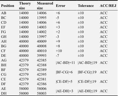
Table 1. Top control data of BZ34-9CEPA jacket. (Unit: mm).
Position Theory size
Measured
size Error Tolerance ACC/REJ
AB 14000 14006 +6 ±10 ACC
BC 14000 13995 -5 ±10 ACC
CD 14000 14006 +6 ±10 ACC
EF 14000 14003 +3 ±10 ACC
FG 14000 14002 +2 ±10 ACC
GH 14000 13997 -3 ±10 ACC
AH 40000 40009 +9 ±10 ACC
BG 40000 40008 +8 ±10 ACC
CF 40000 40010 +10 ±10 ACC
DE 40000 39993 -7 ±10 ACC
AG 42379 42385
|AC-BD|=11 |AC-BD|≤19 ACC BH 42379 42388
BF 42379 42389
|BF-CG|=6 |BF-CG|≤19 ACC CG 42379 42395
CE 42379 42381
|CE-DF|=5 |CE-DF|≤19 ACC DF 42379 42386
AE 58000 58006
|AE-DH|=3 |AE-DH|≤19 ACC DH 58000 58003
2.1.2. Difference Method Characteristics
The advantage of this method is that the principle is simple and easy to operate. The disadvantage is that although this method can judge the simple structure size, the calculated error has no directionality and is not intuitive and reasonable. For complex structures, it is difficult to reflect the deviation of each measurement point, and this method is not conducive to size adjustment at the construction site. It is easy to appear in the field adjustment that the size adjustment in this direction is in place, and the deviation in the other direction is larger, which is not conducive to the size adjustment of the construction personnel. Taking a steel structure in the form of a jacket as an example, if it is necessary to fully reflect the manufacturing error of the steel structure, it needs to be represented by multiple dimensions as shown in Figure 2 [3].
If a certain size exceeds the allowable range of error, adjust this The node needs to consider whether it will affect the adjacent size or diagonal size, etc. The direction and size of the adjustment are difficult to judge.
Figure 2. Schematic diagram of three-dimensional dimensions of steel structure.
2.2. Plane Control Network Method
Planar control network layout is one of the key technologies for the smooth docking of large structures. To ensure the dimensional control quality of large structures, a high-precision plane control network must be established in the construction area [4, 5].
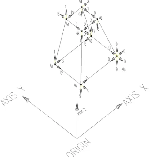
2.2.1. Choosing the Layout of the Plane Control Network Under the premise of fully considering the topographical characteristics of the construction area and the form of the marine steel structure, the plane control network is generally set as a triangular network, as shown in Figure 3 below, and the plane control network is laid out.
2.2.2. Plane Control Network Observation
After the plane control network layout form is determined, the control point observation can be performed. In order to keep consistent with the measurement results of the wiring section, two control points A and B are selected in conjunction with the known point O at the construction site, and the control points A and B can be used as the starting point of the control network. The joint test uses 2 Trimble 5700 GPS receivers and 4 Trimble R8 GNSS receivers to simultaneously
observe 4 time periods in static relative measurement mode. The effective observation time per period is not less than 4 h, the satellite cut-off height angle is not less than 15 °, and the sampling interval is 30 s. The control network observation uses the earth quadrilateral as the basic pattern and is carried out in the form of side connections [6, 7]. Observational technical requirements are linked to known points. Table 2 below shows the measurement results of the control points of the planar control network.
Table 2. Plane Control Network Control Point Measurement Results Table.
Point ID X (m) Y (m)
Starting point measurement result
A 6718.819 3477.589
B 6712.115 3638.101
Plane control point measurement results
C 6847.770 3724.162
D 6990.129 3649.712
E 6996.833 3489.200
F 6861.178 3403.139
2.2.3. Using the Planar Control Network for Dimensional Control and Error Analysis
According to the topographical characteristics of the construction area and the characteristics of the marine steel structure, the appropriate control points are selected as the initial control points for data acquisition [8], and the size control and error analysis of the marine steel structure. Taking
the top size control of the BZ34-9CEPA jacket as an example, according to the line of sight conditions of the site environment and the characteristics of the control network, select control point A, control point C and control point E as the initial control points in the plane control network, and collect data. Data processing is performed, and the size control report is issued as shown in Table 3 below.
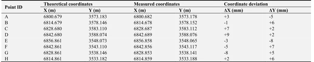
Table 3. BZ34-9CEPA jacket catheter top offset.
Point ID Theoretical coordinates Measured coordinates Coordinate deviation
X (m) Y (m) X (m) Y (m) ∆X (mm) ∆Y (mm)
A 6800.679 3573.183 6800.682 3573.178 +3 -5
B 6814.679 3578.146 6814.678 3578.152 -1 +6
C 6828.680 3583.110 6828.687 3583.112 +7 +2
D 6842.680 3588.074 6842.689 3588.076 +9 +2
E 6856.861 3548.073 6856.858 3548.065 -3 -8
F 6842.861 3543.110 6842.856 3543.117 -5 +7
G 6828.861 3538.146 6828.853 3538.141 -8 +5
H 6814.861 3533.182 6814.859 3533.188 +2 +6
2.2.4. Characteristics of the Observation Method of the Planar Control Network
The advantages of this method:
1)The three-dimensional coordinates of any point to be measured in the coverage area of the control network can be obtained, and the coverage is wide.
2)Comparing with the theoretical value, the offset of the measurement point in three directions can be obtained, and the field worker can be dimensioned to indicate the direction.
3)The data measured by this method has high precision and can be combined with the measurement points around the country.
4)When the site area is large, the control network can be divided into two levels: the first level network and the encryption network [9].
Disadvantages of this method:
1)The principle is complicated. After the data is collected,
professional software is needed for settlement.
2)It takes a long time. A flat control network generally takes 1-3 days to complete, which is not conducive to timely adjustment of the construction site.
3)The cost is higher. The layout of the planar control network requires at least three devices to measure at the same time, and the equipment and dedicated software cost a lot.
3. New Methods for Size Control and
Error Analysis
deviation of each node is reflected objectively and objectively, intuitive and reasonable, and the calculation program is written by AUTOCAD VBA, and the deviation value is quickly calculated, which has a good effect on on-site construction adjustment and error analysis. Still taking the form of the jacket structure as an example, as shown in Figure 4, the deviation values of each node are relative to the theoretical data model. To adjust the position of a three-dimensional space of a point, you only need to adjust the corresponding deviation value in the opposite direction. Since it is based on the least squares method, the total amount of adjustment is minimal.
Figure 4. Schematic diagram of three-dimensional deviation of steel structure.
3.1. Steel Structure Coordinates Fitting Principle
In the actual error analysis of marine steel structure, two-dimensional coordinate fitting is the most common and practical. Now the two-dimensional planar structure is taken as an example to introduce its principle. Firstly, the theoretical model of steel structure needs to be drawn in CAD, so that each node can be obtained. Theoretical coordinates, in order to facilitate analysis, the main axis of the theoretical model is parallel to the axis xor axis yin CAD, assuming that the
theoretical coordinates of each node are (xSi,ySi),i=1, 2,...n. The total coordinates of each node of the steel structure are measured by the total station at the construction site, and the coordinates of each measured point are assumed to be( ,x yi i),i=1, 2,...n . According to the principle of coordinate rotation and translation, the deviation of the measured point from the theoretical coordinate after the coordinate rotation isv vx, y, and then the matrix form of the coordinate transformation is:
0 cos sin
0 sin cos
xi i i
yi i i
v p x x
v q y y
α
α
α
α
− = + − (1)
In the above formula, α is the angle at which the measured coordinates rotate counterclockwise around the Z axis, p q, is the translational component of the axial xdirection and the axial ydirection. And make cosα =u, sinα=w, Then (1) can be expanded to:
xi i i Si
yi i i Si
v p ux wy x v q wx uy y
= + − −
= + + −
(2)
Before the adjustment calculation, the initial value of the parameter p q u w, , , needs to be calculated. Assume that the initial value isp q u w0, 0, 0, 0, in order to calculate the initial value of the parameter, select any corresponding two sets of measured points and theoretical point coordinates [10]. Assume that the coordinates of the two sets of measured points arexk,y x yk, l, l, the theoretical point coordinates of the two groups arexSk,ySk,xSl,ySl, and then there is the following transformation relationship: -1 0 0 0 0 1 0 0 1 = 1 0 0 1
k k Sk
k k Sk
l l Sl
l l Sl
p x y x
q y x y
u x y x
w y x y
− • −
The calculated initial value is p q u w0, 0, 0, 0.
According to the principle of least squares, the sum of all coordinate deviations of the theoretical coordinates and the theoretical coordinates should be minimized [11].
Set 2 2
1
min m
xi yi
i
v v imum
γ =
=
∑
+ = *, meeting the conditionssimultaneously, 2 2 + =1
u w , then correction p q u wˆ ˆ ˆ ˆ, , , can be calculated using indirect adjustment with constraints. The flat difference is the sum of the corrected value and the initial value [12]. 0 0 0 0 ˆ ˆ ˆ ˆ
p p p
q q q
u u u
w w w
= +
= +
= +
= +
At this point, the parameters of the coordinate transformation are calculated, and the deviation value of each node can be calculated according to the formula (2).
3.2. Programming
VBA differs from VB in that VBA requires a host application to run and cannot be used to create standalone applications. VBA automates common processes or processes and creates custom solutions that are best suited to customize existing desktop applications [13].
For the coordinate fitting program of this paper, VBA is
superior to the independent application written by other computer languages. It can omit the input of data, and click on each node instead of the input of data. The operation is very convenient and the execution efficiency is very high. The program running interface is shown in Figure 5:
Figure 5. Coordinate fitting program interface.
3.3. Practical Applications
Before the module is installed at sea, the method can be used for simulation docking, and the deviation value of each docking point can be analyzed and calculated, so that the transition section or the steel pile can be adjusted slightly, thereby reducing the risk of offshore installation. Take the JZ25-1 CEP platform as an example. The project has a total of 8 legs. The A-axis and the B-axis span 40 meters and weigh about 12, 000 tons. Because of the floating method, the top of the jacket is not pulled horizontally. The ribs are connected, and the top of the jacket is easily deformed during transportation and installation. Therefore, it is important to
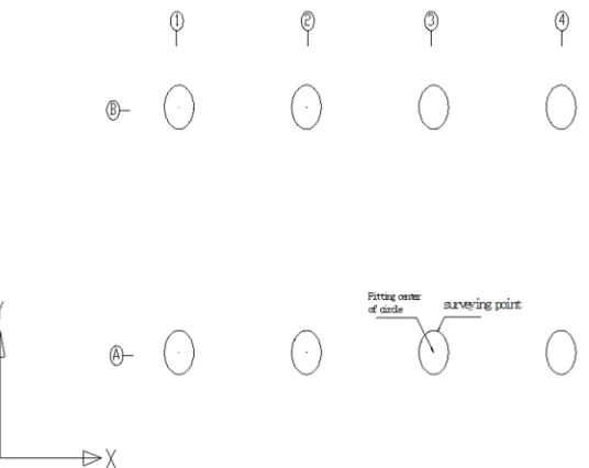
evaluate and adjust the accuracy of the joint before installation. First, after the completion of the module land construction, measure the coordinates of several points on the circumference of each column at the bottom of the module, as shown in Figure 6, and calculate the 8 columns center coordinates of the module using the least squares method [14-15]. The eight center coordinates are used as design data for coordinate fitting. In order to facilitate the calculation of the later deviation analysis, the X-axis of the total station is parallel to the main axis of the module during measurement, and the coordinate data of the center of the bottom of the module column is shown in Table 4.
Table 4. JZ25-1 CEP column and leg column returning structure (LMU) center data table, Unit: mm.
Column ID Center coordinates of each column LMU ID Center coordinates of each LMU
X Y X Y
A1 5464 7826 A1 146044 -10827
A2 19457 7829 A2 147057 -24781
A3 33448 7824 A3 148035 -38749
A4 47446 7826 A4 149044 -52699
B1 5462 47812 B1 185960 -8022
B2 19455 47808 B2 186957 -21962
B3 33459 47812 B3 187954 -35924
B4 47445 47816 B4 188918 -49868
Before installing the module at sea, measure the coordinates of several points on the LUM circle connected to the steel pile on the jacket, and still calculate the best center coordinates of each LUM [14, 15]. The LMU center coordinate data is shown in Table 4.
Using the coordinate fitting method of this paper, the measured 8 LMU center data can best match the 8 column center data at the bottom of the module. The calculation results are shown in Table 5.
Table 5. Coordinate fitting data and deviation value, Unit: mm.
Point ID Module column center data coordinate-converted data of LMU Deviation
X Y X Y △X △Y
A1 5464 7826 5460 7801 -4 -25
A2 19457 7829 19450 7824 -7 -5
A3 33448 7824 33452 7813 +4 -11
A4 47446 7826 47440 7835 -6 +9
B1 5462 47812 5483 47815 +21 +3
B2 19455 47808 19459 47825 +4 +17
B3 33459 47812 33456 47832 -3 +20
B4 47445 47816 47434 47809 -11 -7
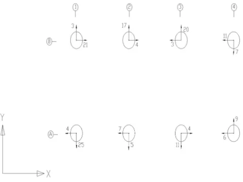
According to the deviation value of Table 5, the deviation diagram of the LMU can be drawn, as shown in Figure 6. According to the docking tolerance error of the project, the risk of installation docking can be evaluated first, and then the corresponding LMU is adjusted accordingly. By applying the method described in this paper, the corresponding LMU is adjusted quickly and accurately to ensure the smooth installation of the LMU.
Figure 7. JZ25-1 LMU deviation data.
3.4. Characteristics of the New Method
By comparing the traditional ocean steel structure error analysis method with the ocean steel structure error analysis method proposed in this paper, the following conclusions can
be drawn:
i. The steel structure error analysis method in this paper is expressed by the deviation size and direction, which is more intuitive and reasonable than the traditional size and length representation. The measurement method uses mathematical analysis to evaluate the error and measure the uncertainty [16].
ii. Using the least squares method to make the best match between the measured data and the design data, to ensure that the sum of all the deviations is the smallest, so the size of the modified steel structure can be greatly reduced, and the construction department can effectively guide the size adjustment. In turn, the construction period of the steel structure is shortened. iii.It plays an important role in the risk assessment and
micro-adjustment of marine steel structure before docking installation. For example, the measured center coordinates of the bottom column of the module are used as design data, and the steel core, transition section, LMU and other structural centers connected with the module are connected. Optimal data matching for measured data. Therefore, the deviation size and direction of each docking point can be visually analyzed. If the deviation exceeds the allowable range, the steel pile, the transition section, the LMU, etc. can be slightly adjusted before the module installation to ensure smooth installation.
4. Conclusions
The dimensional control and error analysis methods described in this paper have their own characteristics, and each has its own applicable conditions. In the case where construction site adjustment is not required, the difference method can be used to quickly obtain the dimensional control result. In the early stage of construction of very large marine steel structures, the layout of planar control nets is the best way to size control. At this stage, the dimensional control and error analysis methods of the marine steel structure construction process are changing from the difference method to the new method, which will achieve the purpose of height adjustment in the field assembly process, greatly reduce the size adjustment time of the construction site, and reduce the labor intensity of workers. Improve work efficiency.
References
[1] Yin Yongqiang, Dong Chao, Wang Jianxi, Wen Hailong. Discussion on the size control of marine steel structure construction process [C]. The 13th China Association for Science and Technology Annual Meeting Ocean Engineering Equipment Development Forum and 2011 Ocean Engineering Academic Annual Meeting Proceedings, 2012, 349-354. [2] Steel structure engineering construction specifications [S].
GB50755-2012.
[3] Yang Yiwei. Discussion on Quality Control of Steel Structure Factory in Construction [J]. Commodity & Quality: Architecture & Development. 2012 (6): 74-74.
[4] Engineering Measurement Specification [S]. GB50026-2007. [5] Lin Yuxiang. Control measurement [M], 2006.
[6] Lai Jinfu, Yang Rui. Discussion on key technology of measurement of first-level control network of bridge engineering [J]. People's Yangtze River. 2015 (14): 73-93. [7] Cheng Zhengfeng, Song Weidong. Control measurement.
Principles and methods of digital mapping., 2009.
[8] Jin Yun. The layout of large bridge elevation control network. Urban road bridge and flood control [M].2009.
[9] Liu Wengu, Zhang Weifu, You Yangsheng. Surveying [M]. 2018.
[10] Department of Measurement and Adjustment, Wuhan University. Measurement Adjustment Foundation. 2007. [11] Department of Mathematics, Tongji University. Advanced
Mathematics. 2007.
[12] Tao Benzao, Qiu Weining, Huang Gana. Error Theory and Measurement Adjustment Foundation [M]. Wuhan: Wuhan University Press, 2003: 102-148.
[13] Zhang Shijian, Liu Chunjie. A New Method for Accurate Measurement of Steel Pile Span of Jacket Frame [J], 2014, 26 (5): 92-95.
[14] Liu Chunjie, Zhang Shijian. A method for detecting the overall size of jackets [J]. Surveying Engineering, 2014, 23 (2): 39-44. [15] Liu Chunjie, Zhang Shijian, Sun Yunhu. Method for detecting the spatial position of circular members of jackets in three-dimensional coordinate system [P], ZL201010115279.X. November 28, 2012.