Preventing Over-Fitting during Model Selection via Bayesian Regularisation of the Hyper-Parameters

Preventing Over-Fitting during Model Selection via Bayesian

Regularisation of the Hyper-Parameters

Gavin C. Cawley [email protected]

Nicola L. C. Talbot [email protected]

School of Computing Sciences University of East Anglia

Norwich, United Kingdom NR4 7TJ

Editors: Isabelle Guyon and Amir Saffari

Abstract

While the model parameters of a kernel machine are typically given by the solution of a convex op-timisation problem, with a single global optimum, the selection of good values for the regularisation and kernel parameters is much less straightforward. Fortunately the leave-one-out cross-validation procedure can be performed or a least approximated very efficiently in closed form for a wide vari-ety of kernel learning methods, providing a convenient means for model selection. Leave-one-out cross-validation based estimates of performance, however, generally exhibit a relatively high vari-ance and are therefore prone to over-fitting. In this paper, we investigate the novel use of Bayesian regularisation at the second level of inference, adding a regularisation term to the model selection criterion corresponding to a prior over the hyper-parameter values, where the additional regulari-sation parameters are integrated out analytically. Results obtained on a suite of thirteen real-world and synthetic benchmark data sets clearly demonstrate the benefit of this approach.

Keywords: model selection, kernel methods, Bayesian regularisation

1. Introduction

Leave-one-out cross-validation (Lachenbruch and Mickey, 1968; Luntz and Brailovsky, 1969; Stone, 1974) provides the basis for computationally efficient model selection strategies for a variety of ker-nel learning methods, including the Support Vector Machine (SVM) (Cortes and Vapnik, 1995; Chapelle et al., 2002), Gaussian Process (GP) (Rasmussen and Williams, 2006; Sundararajan and Keerthi, 2001), Least-Squares Support Vector Machine (LS-SVM) (Suykens and Vandewalle, 1999; Cawley and Talbot, 2004), Kernel Fisher Discriminant (KFD) analysis (Mika et al., 1999; Caw-ley and Talbot, 2003; Saadi et al., 2004; Bo et al., 2006) and Kernel Logistic Regression (KLR) (Keerthi et al., 2005; Cawley and Talbot, 2007). These methods have proved highly successful for kernel machines having only a small number of hyper-parameters to optimise, as demonstrated by the set of models achieving the best average score in the WCCI-2006 performance prediction challenge1(Cawley, 2006; Guyon et al., 2006). Unfortunately, while leave-one-out cross-validation estimators have been shown to be almost unbiased (Luntz and Brailovsky, 1969), they are known to exhibit a relatively high variance (e.g., Kohavi, 1995). A kernel with many hyper-parameters, for instance those used in Automatic Relevance Determination (ARD) (e.g., Rasmussen and Williams, 2006) or feature scaling methods (Chapelle et al., 2002; Bo et al., 2006), may provide sufficient

degrees of freedom to over-fit leave-one-out cross-validation based model selection criteria, result-ing in performance inferior to that obtained usresult-ing a less flexible kernel function. In this paper, we investigate the novel use of regularisation (Tikhonov and Arsenin, 1977) of the hyper-parameters in model selection in order to ameliorate the effects of the high variance of leave-one-out cross-validation based selection criteria, and so improve predictive performance. The regularisation term corresponds to a zero-mean Gaussian prior over the values of the kernel parameters, representing a preference for smooth kernel functions, and hence a relatively simple classifier. The regularisation parameters introduced in this step are integrated out analytically in the style of Buntine and Weigend (1991), to provide a Bayesian model selection criterion that can be optimised in a straightforward manner via, for example, scaled conjugate gradient descent (Williams, 1991).

The paper is structured as follows: The remainder of this section provides a brief overview of the least-squares support vector machine, including the use of leave-one-out cross-validation based model selection procedures, given in sufficient detail to ensure the reproducibility of the results. Section 2 describes the use of Bayesian regularisation to prevent over-fitting at the second level of inference, that is, model selection. Section 3 presents results obtained over a suite of thirteen benchmark data sets, which demonstrate the utility of this approach. Section 4 provides discussion of the results and suggests directions for further research. Finally, the work is summarised and directions for further work are outlined in Section 5.

1.1 Least Squares Support Vector Machine

In the remainder of this section, we provide a brief overview of the least-squares support vector machine (Suykens and Vandewalle, 1999) used as the testbed for the investigation of the role of regularisation in the model selection process described in this study. Given training data,

D

=_{(xi,yi)}`i=1, where xi∈

X

⊂Rd and yi∈ {−1,+1},

we seek to construct a linear discriminant, f(x) =φ(x)_·w+b, in a feature space,

F

, defined by a fixed transformation of the input space, φ:

X

_→

F

. The parameters of the linear discriminant, (w, b), are given by the minimiser of a regularised (Tikhonov and Arsenin, 1977) least-squares training criterion,

L=1 2kwk

2₊ 1 2µ

`

∑

i=1

[yi−φ(xi)·w−b]2, (1)

where µ is a regularisation parameter controlling the bias-variance trade-off (Geman et al., 1992). Rather than specify the feature space directly, it is instead induced by a kernel function,

K

:

X

_×

X

_→

R, which evaluates the inner-product between the projections of the data onto the feature space,

F

, that is,

K

(x,x0) =φ(x)_·φ(x0). The interpretation of an inner-product in a fixed feature space is valid for any Mercer kernel (Mercer, 1909), for which the Gram matrix, K= [ki j=

K

(xi,xj)]`_i,j=1 is positive semi-definite, that is,

aTKa_≥0, _∀a_∈R`, a₆=0.

and Wahba, 1971) shows that the solution of the optimisation problem (1) can be written as an expansion over the training patterns,

w= `

∑

i=1

αiφ(xi) =⇒ f(x) =

`

∑

i=1

αi

K

(xi,x) +b.

The advantage of the “kernel trick” then becomes apparent; a linear model can be constructed in an extremely rich, high- (possibly infinite-) dimensional feature space, using only finite-dimensional quantities, such as the Gram matrix, K. The “kernel trick” also allows the construction of statistical models that operate directly on structured data, for instance strings, trees and graphs, leading to the current interest in kernel learning methods in computational biology (Sch ¨olkopf et al., 2004) and text-processing (Joachims, 2002). The Radial Basis Function (RBF) kernel,

K

(x,x0) =exp−ηkx−x0k2

is commonly encountered in practical applications of kernel learning methods, here ηis a kernel parameter, controlling the sensitivity of the kernel function. The feature space for the radial basis function kernel consists of the positive orthant of an infinite-dimensional unit hyper-sphere (e.g., Shawe-Taylor and Cristianini, 2004). The Gram matrix for the radial basis function kernel is thus of full rank (Micchelli, 1986), and so the kernel model is able to form an arbitrary shattering of the data.

1.1.1 A DUALTRAININGALGORITHM

The basic training algorithm for the least-squares support vector machine (Suykens and Vandewalle, 1999) views the regularised loss function (1) as a constrained minimisation problem:

min w,b,εi

1 2kwk

2₊ 1 2µ

`

∑

i=1 ε2

i subject to εi=yi−w·φ(xi)−b.

The primal Lagrangian for this constrained optimisation problem gives the unconstrained minimi-sation problem defined by the following regularised loss function,

L

=1

2kwk 2₊ 1

2µ `

∑

i=1 ε2

i −

`

∑

i=1

αi{w·φ(xi) +b+εi−yi},

whereα= (α1,α2, . . . ,α`)∈R`is a vector of Lagrange multipliers. The optimality conditions for this problem can be expressed as follows:

∂

L

∂w = 0 =⇒ w= `

∑

i=1

αiφ(xi), (2)

∂

L

∂b = 0 =⇒ `

∑

i=1

αi=0, (3)

∂

L

∂εi

= 0 =_⇒ αi=

εi

µ, ∀i∈ {1,2, . . . , `}, (4) ∂

L

∂αi

Using (2) and (4) to eliminate w andε= (ε1,ε2, . . . ,ε`), from (5), we find that `

∑

j=1

αjφ(xj)·φ(xi) +b+µαi=yi ∀i∈ {1,2, . . . , `}. (6)

Noting that

K

(x,x0) =φ(x)_·φ(x0_{), the system of linear equations, (6) and (3), can be written more} concisely in matrix form as

K+µI 1 1T 0

α b

=

y 0

,

where K= [ki j=

K

(xi,xj)]_i`<sub>,j=1</sub>, I is the`×`identity matrix and 1 is a column vector of`ones. The optimal parameters for the model of the conditional mean can then be obtained with a computational complexity of

O

(`3_{)operations, using direct methods, such as Cholesky decomposition (Golub and} Van Loan, 1996).

1.1.2 EFFICIENTIMPLEMENTATIONVIACHOLESKYDECOMPOSITION

A more efficient training algorithm can be obtained, taking advantage of the special structure of the system of linear equations (Suykens et al., 2002). The system of linear equations to be solved in fitting a least-squares support vector machine is given by,

M 1 1T 0

_α

b

=

y 0

, (7)

where M=K+µI. Unfortunately the matrix on the left-hand side is not positive definite, and so we cannot solve this system of linear equations directly using the Cholesky decomposition. However, the first row of (7) can be re-written as

M α+M−11b=y. (8)

Rearranging (8), we see thatα=M−1(y₋1b), using this result to eliminateα, the second row of (7) can be written as

1TM−11b=1TM−1y. The system of linear equations can then be re-written as

M 0

0T 1TM−11

_α

+M−11b b

=

y 1TM−1y

. (9)

In this case, the matrix on the left hand side is positive-definite, as M=K+λI is positive-definite and 1TM−11 is positive since the inverse of a positive definite matrix is also positive definite. The revised system of linear equations (9) can be solved as follows: First solve

Mρ=1 and Mν=y, (10)

which may be performed efficiently using the Cholesky factorisation of M. The model parameters of the least-squares support vector machine are then given by

b=1 T_ν

1Tρ and α=ν−ρb.

1.2 Leave-One-Out Cross-Validation

Cross-validation (Stone, 1974) is commonly used to obtain a reliable estimate of the test error for performance estimation or for use as a model selection criterion. The most common form, k-fold cross-validation, partitions the available data into k disjoint subsets. In each iteration a classifier is trained on a different combination of k₋1 subsets and the unused subset is used to estimate the test error rate. The k-fold cross-validation estimate of the test error rate is then simply the av-erage of the test error rate observed in each of the k iterations, or folds. The most extreme form of cross-validation, where k=` such that the test partition in each fold consists of only a sin-gle pattern, is known as leave-one-out cross-validation (Lachenbruch and Mickey, 1968) and has been shown to provide an almost unbiased estimate of the test error rate (Luntz and Brailovsky, 1969). Leave-one-out cross-validation is however computationally expensive, in the case of the least-squares support vector machine a na¨ıve implementation having a complexity of

O

(`4₎ opera-tions. Leave-one-out cross-validation is therefore normally only used in circumstances where the available data are extremely scarce such that the computational expense is no longer prohibitive. In this case the inherently high variance of the leave-one-out estimator (Kohavi, 1995) is offset by the minimal decrease in the size of the training set in each fold, and so may provide a more reliable estimate of generalisation performance than conventional k-fold cross-validation. Fortunately leave-one-out cross-validation of least-squares support vector machines can be performed in closed form with a computational complexity of only

O

(`3_{)operations (Cawley and Talbot, 2004).} Leave-one-out cross-validation can then be used in medium to large scale applications, where there may be a few thousand data-points, although the relatively high variance of this estimator remains potentially problematic.

1.2.1 VIRTUALLEAVE-ONE-OUT CROSS-VALIDATION

The optimal values of the parameters of a Least-Squares Support Vector Machine are given by the solution of a system of linear equations:

K+µI 1 1T 0

_α

b

=

y 0

. (11)

The matrix on the left-hand side of (11) can be decomposed into block-matrix representation, as

follows:

K+µI 1 1T 0

=

c11 cT₁ c1 C1

=C.

Let[α(−i)_{; b}(−i)_{]represent the parameters of the least-squares support vector machine during the i}th iteration of the leave-one-out cross-validation procedure, then in the first iteration, in which the first training pattern is excluded,

_α(−1)

b(−1)

=C−₁1[y2, . . . ,y`,0]T. The leave-one-out prediction for the first training pattern is then given by

ˆ

y(₁−1)=cT₁

_α(−1)

b(−1)

Considering the last ` equations in the system of linear equations (11), it is clear that [c1C1] [α1, . . . ,α`,b]T = [y2, . . . ,y`,0]T, and so

ˆ

y₁(−1)=cT₁C₁−1[c1C1]αT,bT=cT₁C−₁1c1α1+c1[α2, . . . ,α`,b]T.

Noting, from the first equation in the system of linear equations (11), that y1 = c11α1+ cT₁[α2, . . . ,α`,b]T, thus

ˆ

y(₁−1)=y1−α1 c11−cT1C−11c1

.

Finally, via the block matrix inversion lemma,

c11 cT₁ c1 C1

−1 =

_κ−1

−κ−1_c1C−1 1 C−₁1+κ−1_C−1

1 cT1c1C−11 −κ−1C−11cT1

,

whereκ=c11−cT1C−11c, and noting that the system of linear equations (11) is insensitive to permu-tations of the ordering of the equations and of the unknowns, we have that,

yi−yˆ(i−i)=

αi

C−_ii1. (12)

This means that, assuming the system of linear equations (11) is solved via explicit inversion of C, a leave-one-out cross-validation estimate of an appropriate model selection criterion can be evalu-ated using information already available a by-product of training the least-squares support vector machine on the entire data set (cf., Sundararajan and Keerthi, 2001).

1.2.2 EFFICIENTIMPLEMENTATION VIACHOLESKYFACTORISATION

The leave-one-out cross-validation behaviour of the least-squares support vector machine is de-scribed by (12). The coefficients of the kernel expansion,α, can be found efficiently, via Cholesky factorisation, as described in Section 1.1.2. However we must also determine the diagonal elements of C−1in an efficient manner. Using the block matrix inversion formula, we obtain

C−1=

M 1 1T 0

₋1 =

M−1+M−11S−_M11TM−1 ₋M−11S_M−1

−S−_M11TM−1 S−_M1

where M=K+µI and SM=−1TM−11=−1Tηis the Schur complement of M. The inverse of the positive definite matrix, M, can be computed efficiently from its Cholesky factorisation, via the SYMINValgorithm (Seaks, 1972), for example using the LAPACK routineDTRTRI(Anderson et al., 1999). Let R= [ri j]`_i,j=1 be the lower triangular Cholesky factor of the positive definite matrix M, such that M=RRT. Furthermore, let

S= [si j]`_i,j=1=R−1, where sii= 1 rii

and si j=−sii i−1

∑

k=1 riksk j,

represent the (lower triangular) inverse of the Cholesky factor. The inverse of M is then given by M−1=STS. In the case of efficient leave-one-out cross-validation of least-squares support vector machines, we are principally concerned only with the diagonal elements of M−1, given by

M_ii−1= i

∑

j=1

s2_{i j} =_⇒ C_ii−1= i

∑

j=1 s2_{i j}+ρ

2 i SM ∀

The computational complexity of the basic training algorithm is

O

(`3_{)operations, being} dom-inated by the evaluation of the Cholesky factor. However, the computational complexity of the analytic leave-one-out cross-validation procedure, when performed as a by-product of the training algorithm, is only

O

(`)operations. The computational expense of the leave-one-out cross-validation procedure therefore becomes increasingly negligible as the training set becomes larger.

1.3 Model Selection

The virtual leave-one-out cross-validation procedure described in the previous section provides the basis for a simple automated model selection strategy for the least-squares support vector machine. Perhaps the most basic model selection criterion is provided by the Predicted REsidual Sum of Squares (PRESS) criterion (Allen, 1974), which is simply the leave-one-out estimate of the sum-of-squares error,

Q(θ) =1 2

`

∑

i=1

h

yi−yˆ(i−i)

i2 .

A minimum of the model selection criterion is often found via a simple grid-search procedure in the majority of practical applications of kernel learning methods. However, this is rarely necessary and often highly inefficient as a grid-search spends a large amount of time investigating hyper-parameter values outside the neighbourhood of the global optimum. A more efficient approach uses the Nelder-Mead simplex algorithm (Nelder and Mead, 1965), as implemented by thefminsearch function of the MATLAB optimisation toolbox. An alternative easily implemented approach uses conjugate gradient methods, with the required gradient information estimated by the method of finite differences, and implemented by thefminunc function from the MATLAB optimisation toolbox. In this study however, we use scaled conjugate gradient descent (Williams, 1991), with the required gradient information evaluated analytically, as this is approximately twice as efficient.

1.3.1 PARTIALDERIVATIVES OF THEPRESS MODELSELECTIONCRITERION

Letθ=_{θ1, . . . ,θn}={λ,η1, . . . ,ηd}represent the vector of hyper-parameters for a least-squares support vector machine, where η1, . . . ,ηd represent the kernel parameters. The PRESS statistic (Allen, 1974) can be written as

Q(θ) = 1 2

`

∑

i=1

h

r(_i−i)

i2

, where r_i(−i)=yi−yˆ(i−i)=

αi C_ii−1.

Using the chain rule, the partial derivative of the PRESS statistic, with respect to an individual hyper-parameter,θj, is given by,

∂Q(θ) ∂θj

= `

∑

i=1 ∂Q(θ)

∂r_i(−i) ∂r_i(−i)

∂θj

,

where

∂Q(θ) ∂r(_i−i)

=r(_i−i)= αi

C−_ii1 and

∂r(_i−i) ∂θj

= ∂αi ∂θj

1 C−_ii1−

αi

C−_ii12 ∂C−_ii1

∂θj

,

such that

∂Q(θ) ∂θj

= `

∑

i=1 αi C−_ii1

(

∂αi

∂θj 1 C−_ii1−

αi

C−_ii12 ∂C−_ii1

∂θj

)

We begin by deriving the partial derivatives of the model parameters, αT bT, with respect to the hyper-parameterθj. The model parameters are given by the solution of a system of linear equations,

such that

αT _bT _=C−1_yT ₀T_.

Using the following identity for the partial derivatives of the inverse of a matrix,

∂C−1 ∂θj

=₋C−1∂C ∂θj

C−1, (13)

we obtain,

∂αT _bT

∂θj

=₋C−1_∂θ∂C j

C−1yT 0=₋C−1_∂θ∂C j

_αT

bT.

Note the computational complexity of evaluating the partial derivatives of the model parameters is

O

(`2_{), as only two successive matrix-vector products are required. The partial derivatives of the} diagonal elements of C−1can be found using the inverse matrix derivative identity (13). For a kernel parameter,∂C/∂ηjwill generally be fully dense, and so the computational complexity of evaluating the diagonal elements of∂C−1/∂ηjwill be

O

(`3)operations. If, on the other hand, we consider the regularisation parameter, µ, we have that

∂C ∂µ =

I 0 0T 0

,

and so the computation of the partial derivatives of the model parameters, with respect to the regu-larisation parameter, is slightly simplified,

∂αT _bT

∂µ =−C

−1_αT _bT_.

More importantly, as ∂C/∂µ is diagonal, the diagonal elements of (13) can be evaluated with a computational complexity of only

O

(`2_{) operations. This suggests that it may be more efficient} to adopt different strategies for optimising the regularisation parameter, µ, and the vector of kernel parameters,η, (cf., Saadi et al., 2004). For a kernel parameter,ηj, the partial derivatives of C with respect toηjare given by the partial derivatives of the kernel matrix, that is,

∂C ∂ηj

=

_∂

K/∂ηj 0 0T 0

.

For the spherical radial basis function kernel, used in this study, the partial derivative with respect to the kernel parameter is given by

∂

K

(x,x0)

∂η =−

K

(x,x0)kx−x0k2.

Finally, since the regularisation parameter, µ, and the scale parameter of the radial basis function kernel are strictly positive quantities, in order to permit the use of an unconstrained optimisation procedure, we adopt the parameterisationeθj=log2θj, such that

∂Q(θ) ∂e_θj =

∂Q(θ) ∂θj

∂θj

∂e_θj where

∂θj

1.3.2 AUTOMATICRELEVANCEDETERMINATION

Automatic Relevance Determination (ARD) (e.g., Rasmussen and Williams, 2006), also known as feature scaling (Chapelle et al., 2002; Bo et al., 2006), aims to identify informative input features as a natural consequence of optimising the model selection criterion. This can be most easily achieved using an elliptical radial basis function kernel,

K

(x,x0) =exp

( −

d

∑

i=1

ηi[xi−x0i]2

)

,

that incorporates individual scaling factors for each input dimension. The partial derivatives with respect to the kernel parameters are then given by,

∂

K

(x,x0) ∂ηi

=₋

K

(x,x0)[xi−x0i]2.

Generalisation performance is likely to be enhanced if irrelevant features are down-weighted. It is therefore hoped that minimising the model selection criterion will lead to very small values for the scaling factors associated with redundant input features, allowing them to be identified and pruned from the model.

2. Bayesian Regularisation in Model Selection

In order to overcome the observed over-fitting in model selection using leave-one-out cross-validation based methods, we propose to add a regularisation term (Tikhonov and Arsenin, 1977) to the model selection criterion, which penalises solutions where the kernel parameters take on unduly large val-ues. The regularised model selection criterion is then given by

M(θ) =ζQ(θ) +ξΩ(θ), (14)

whereξandζare additional regularisation parameters, Q(θ)is the model selection criterion, in this case the PRESS statistic andΩ(θ)is a regularisation term,

Q(θ) =1 2

`

∑

i=1

h

yi−yˆ(i−i)

i2

and Ω(θ) =1 2

d

∑

i=1 η2

i.

In this study we have left the regularisation parameter, µ, unregularised. However, we have now introduced two further regularisation parametersξandζfor which good values must also be found. This problem may be solved by taking a Bayesian approach and adopting an ignorance prior and integrating out the additional regularisation parameters analytically in the style of Buntine and Weigend (1991). Adapting the approach taken by Williams (1995), the regularised model selec-tion criterion (14) can be interpreted as the posterior density in the space of the hyper-parameters,

P(θ_|

D

)∝P(

D

_|θ)P(θ),

hyper-parameters, in this case that they should have a small magnitude, corresponding to a relatively simple model. These quantities can be expressed as

P(

D

_|θ) =Z_Q−1exp_{−ζQ(θ)_} and P(θ) =Z_Ω−1exp_{−ξΩ(θ)_}

where ZQand ZΩ are the appropriate normalising constants. Assuming the data represent an i.i.d. sample, the likelihood in this case is Gaussian,

P(

D

_|θ) = `

∏

i=1 1

√

2πσexp

  

 −

h

yi−yˆ(i−i)

i2 2σ2

  



 where ζ=

1

σ2 =⇒ ZQ=

2π ζ

`/2 .

Likewise, the prior is a Gaussian, centred on the origin,

P(θ) = d

∏

i=1 1

p

2π/ξexp

−ξ

2η 2 i

such that Z_Ω=

2π ξ

d/2 .

Minimising (14) is thus equivalent to maximising the posterior density with respect to the hyper-parameters. Note that the use of a prior over the hyper-parameters is in accordance with normal Bayesian practice and has been investigated in the case of Gaussian Process classifiers by Williams and Barber (1998). The combination of frequentist and Bayesian approaches at the first and sec-ond levels of inference is however somewhat unusual. The marginal likelihood is dependent on the assumptions of the model, which may not be completely appropriate. Cross-validation based procedures may therefore be more robust in the case of model mis-specification (Wahba, 1990). It seems reasonable for the model to be less sensitive to assumptions at the second level of inference than the first, and so the proposed approach represents a pragmatic combination of techniques.

2.1 Elimination of Second Level Regularisation Parametersξandζ

Under the evidence framework proposed by MacKay (1992a,b,c) the hyper-parametersξandζare determined by maximising the marginal likelihood, also known as the Bayesian evidence for the model. In this study, however we opt to integrate out the hyper-parameters analytically, extending the work by Buntine and Weigend (1991) and Williams (1995) to consider Bayesian regularisation at the second level of inference, namely the selection of good values for the hyper-parameters. We begin with the prior over the hyper-parameters, which depends onξ,

P(θ_|ξ) =ZΩ(ξ)−1exp_{−ξΩ_}.

The regularisation parameterξmay then be integrated out analytically using a suitable prior, P(ξ),

P(θ) = Z

P(θ_|ξ)P(ξ)dξ.

The improper Jeffreys’ prior, P(ξ)∝1/ξis an appropriate ignorance prior in this case asξis a scale parameter, noting thatξis strictly positive,

p(θ) = 1 (2π)d/2

Z ∞ 0 ξ

Using the Gamma integralR∞

0 xν−1e−µxdx=Γ(ν)/µν(Gradshteyn and Ryzhic, 1994, equation 3.384), we obtain

p(θ) = 1 (2π)d/2

Γ(d/2)

Ωd/2 =⇒ −log p(θ)∝ d 2logΩ.

Finally, adopting a similar procedure to eliminateζ, we obtain a revised model selection criterion with Bayesian regularisation,

L= `

2log Q(θ) + d

2logΩ(θ). (15)

in which the regularisation parameters have been eliminated. As before, this criterion can be opti-mised via standard methods, such as the Nelder-Mead simplex algorithm (Nelder and Mead, 1965) or scaled conjugate gradient descent (Williams, 1991). The partial derivatives of the proposed Bayesian model selection criterion are given by

∂L ∂θi

= `

2Q(θ) ∂Q(θ)

∂θi

+ d

2Ω(θ) ∂Ω(θ)

∂θi

and ∂Ω(θ) ∂ηi

=ηi.

The additional computational expense involved in Bayesian regularisation of the model selection criterion is only

O

(d)operations, and is extremely small in comparison with the

O

(`3_)operations involved in obtaining the leave-one-out error (including the cost of training the model on the entire data set). Per iteration of the model selection process, the cost of the Bayesian regularisation is therefore minimal. There seems little reason to suppose that the regularisation will have an adverse effect on convergence, and this seems to be the case in practice.

2.2 Relationship with the Evidence Framework

Under the evidence framework of MacKay (1992a,b,c) the regularisation parameters,ξandζ, are selected so as to maximise the marginal likelihood, also known as the Bayesian evidence, for the model. The log-evidence is given by

log P(

D

) =₋ξΩ(θ)₋ζQ(θ)₋1

2log|A|+ d 2logξ+

` 2logζ−

`

2log{2π},

where A is the Hessian of the regularised model selection criterion (14) with respect to the hyper-parameters,θ. Setting the partial derivatives of the log evidence with respect to the regularisation parameters,ξandζ, equal to zero, we obtain the familiar update formulae,

ξnew₌ γ

2Ω(θ) and ζ

new₌ `−γ 2Q(θ),

whereγis the number of well defined hyper-parameters, that is, the hyper-parameters for which the optimal value is primarily determined by the log-likelihood term, Q(θ)rather than by the regulariser, Ω(θ). In the case of the L2 regularisation term, corresponding to a Gaussian prior, the number of well determined hyper-parameters is given by

γ= n

∑

j=1 λj

λj+ξ

Bayesian regularisation scheme is equivalent to optimising the regularised model selection criterion (14) assuming that the regularisation parameters,ξandζ, are continuously updated according to the following update rules,

ξeff₌ d

2Ω(θ) and ζ

eff₌ ` 2Q(θ).

This exactly corresponds to the “cheap and cheerful” approximation of the evidence framework sug-gested by MacKay (1994), which assumes that all of the hyper-parameters are well-determined and that the number of hyper-parameters is small in relation to the number of training patterns. Since γ≤d, it seems self evident that the proposed Bayesian regularisation scheme will be prone to a de-gree of under-fitting, especially in the case of a feature scaling kernel with many redundant features. The theoretical and practical pros and cons of the integrate-out approach and the evidence frame-work are discussed in some detail by MacKay (1994) and Bishop (1995) and references therein. However, the integrate-out approach does not require the evaluation of the Hessian matrix of the original selection criterion, Q(θ), which is likely to prove computationally prohibitive.

3. Results

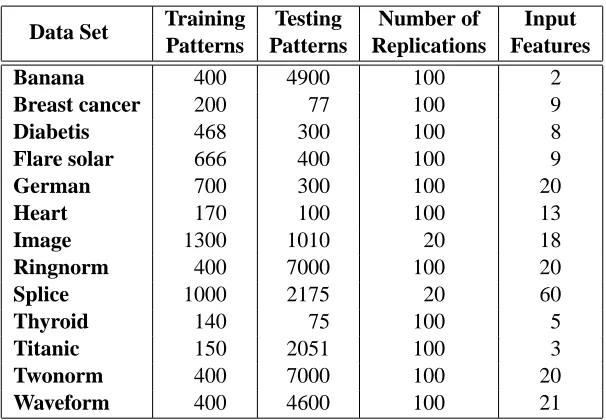
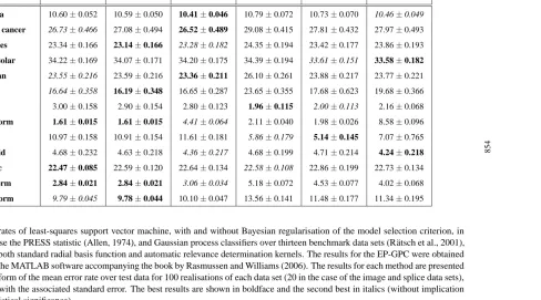
In this section, we present experimental results demonstrating the benefits of the proposed model selection strategy incorporating Bayesian regularisation to overcome the inherent high variance of leave-one-out cross-validation based selection criteria. Table 2 shows a comparison of the error rates of least-squares support vector machines, using model selection procedures with, and without, Bayesian regularisation, (LS-SVM and LS-SVM-BR respectively) over the suite of thirteen pub-lic domain benchmark data sets used in the study by Mika et al. (2000). Results obtained using a Gaussian process classifier (Rasmussen and Williams, 2006), based on the expectation propagation method, are also provided for comparison (EP-GPC). The same set of 100 random partitions of the data (20 in the case of the largerimageandsplicebenchmarks) to form training and test sets used in that study are also used here. In each case, model selection is performed independently for each realisation of the data set, such that the standard errors reflect the variability of both the training algorithm and the model selection procedure with changes in the sampling of the data. Both con-ventional spherical and elliptical radial basis kernels are used for all kernel learning methods, so that the effectiveness of each algorithm for automatic relevance determination can be assessed. The use of multiple training/test partitions allows an estimate of the statistical significance of differences in performance between algorithms to be computed. Let ˆx and ˆy represent the means of the perfor-mance statistic for a pair of competing algorithms, and exand eythe corresponding standard errors, then the z statistic is computed as

z=qyˆ−xˆ

e2 x+e2y

.

The z-score can then be converted to a significance level via the normal cumulative distribution function, such that z=1.64 corresponds to a 95% significance level. All statements of statistical significance in the remainder of this section refer to a 95% level of significance.

3.1 Performance of Models Based on the Spherical RBF Kernel

Data Set Training Testing Number of Input Patterns Patterns Replications Features

Banana 400 4900 100 2

Breast cancer 200 77 100 9

Diabetis 468 300 100 8

Flare solar 666 400 100 9

German 700 300 100 20

Heart 170 100 100 13

Image 1300 1010 20 18

Ringnorm 400 7000 100 20

Splice 1000 2175 20 60

Thyroid 140 75 100 5

Titanic 150 2051 100 3

Twonorm 400 7000 100 20

Waveform 400 4600 100 21

Table 1: Details of data sets used in empirical comparison.

LS-SVM models with and without Bayesian regularisation are very similar, with neither model proving significantly better than the other on any of the data sets. This seems reasonable given that only two hyper-parameters are optimised during model selection and so there is little scope for over-fitting the PRESS model selection criterion and the regularisation term will have little effect. The LS-SVM model with Bayesian regularisation is significantly out-performed by the Gaussian Process classifier on one benchmark banana, but performs significantly better on a further four (ringnorm, splice,twonorm,waveform). Demˇsar (2006) recommends the use of the Wilcoxon signed rank test for assessing the statistical significance of differences in performance over multiple data sets. According to this test, neither the LSSVM-BR nor the EP-PGC is statistically superior at the 95% level of significance.

3.2 Performance of Models Based on the Elliptical RBF Kernel

C

A

W

L

E

Y

A

N

D

T

A

L

B

O

T

Banana 10.60_±0.052 10.59_±0.050 10.41_±0.046 10.79_±0.072 10.73_±0.070 10.46_±0.049

Breast cancer 26.73_±0.466 27.08_±0.494 26.52_±0.489 29.08_±0.415 27.81_±0.432 27.97_±0.493

Diabetes 23.34_±0.166 23.14_±0.166 23.28_±0.182 24.35_±0.194 23.42_±0.177 23.86_±0.193

Flare solar 34.22_±0.169 34.07_±0.171 34.20_±0.175 34.39_±0.194 33.61_±0.151 33.58_±0.182 German 23.55_±0.216 23.59_±0.216 23.36_±0.211 26.10_±0.261 23.88_±0.217 23.77_±0.221

Heart 16.64_±0.358 16.19_±0.348 16.65_±0.287 23.65_±0.355 17.68_±0.623 19.68_±0.366

Image 3.00_±0.158 2.90_±0.154 2.80_±0.123 1.96_±0.115 2.00_±0.113 2.16_±0.068

Ringnorm 1.61_±0.015 1.61_±0.015 4.41_±0.064 2.11_±0.040 1.98_±0.026 8.58_±0.096

Splice 10.97_±0.158 10.91_±0.154 11.61_±0.181 5.86_±0.179 5.14_±0.145 7.07_±0.765

Thyroid 4.68_±0.232 4.63_±0.218 4.36_±0.217 4.68_±0.199 4.71_±0.214 4.24_±0.218 Titanic 22.47_±0.085 22.59_±0.120 22.64_±0.134 22.58_±0.108 22.86_±0.199 22.73_±0.134

Twonorm 2.84_±0.021 2.84_±0.021 3.06_±0.034 5.18_±0.072 4.53_±0.077 4.02_±0.068

Waveform 9.79_±0.045 9.78_±0.044 10.10_±0.047 13.56_±0.141 11.48_±0.177 11.34_±0.195

Table 2: Error rates of least-squares support vector machine, with and without Bayesian regularisation of the model selection criterion, in this case the PRESS statistic (Allen, 1974), and Gaussian process classifiers over thirteen benchmark data sets (R ¨atsch et al., 2001), using both standard radial basis function and automatic relevance determination kernels. The results for the EP-GPC were obtained using the MATLAB software accompanying the book by Rasmussen and Williams (2006). The results for each method are presented in the form of the mean error rate over test data for 100 realisations of each data set (20 in the case of the image and splice data sets), along with the associated standard error. The best results are shown in boldface and the second best in italics (without implication of statistical significance).

imageandsplice), while being significantly worse on six (breast cancer, diabetis,heart, ringnorm,twonormandwaveform).

In the case of the elliptical RBF kernel, the use of Bayesian regularisation in model selection has a dramatic effect on the performance of LS-SVM models, with the LS-SVM-BR model prov-ing significantly better than the conventional LS-SVM on nine of the thirteen benchmarks (breast cancer,diabetis, flare solar, german,heart,ringnorm,splice, twonormandwaveform) without being significantly worse on any of the remaining four data sets. This demonstrates that over-fitting in model selection, due to the larger number of kernel parameters, is likely to be the significant factor causing the relatively poor performance of models with the elliptical RBF kernel. Again, the Gaussian Process classifier is significantly better than the LS-SVM with Bayesian regu-larisation on thebananaandtwonormdata sets, but is significantly worse on four of the remaining eleven (diabetis,heart,ringnormandsplice). Again, according to the Wilcoxon signed rank test, neither the LSSVM-BR nor the EP-PGC is statistically superior at the 95% level of signifi-cance. However the magnitude of the difference in performance between LSSVM-BR and EP-GPC approaches tends to be greatest when the LSSVM-BR out-performs EP-GPC, most notably on the heart,spliceandringnormdata sets. This provides some support for the observation of Wahba (1990) that cross-validation based model selection procedures should be more robust against model mis-specification (see also Rasmussen and Williams, 2006).

4. Discussion

The experimental evaluation presented in the previous section demonstrates that over-fitting can occur in model selection, due to the variance of the model selection criterion. In many cases the minimum of the selection criterion using the elliptical RBF kernel is lower than that achievable us-ing the spherical RBF kernel, however this results in a degradation in generalisation performance. Using the PRESS statistic, the over-fitting is likely to be most severe in cases with a small num-ber of training patterns, as the variance of the leave-one-out estimator decreases as the sample size becomes larger. Using the standard LSSVM, the elliptical RBF kernel only out-performs the spher-ical RBF kernel on two of the thirteen data sets,imageandsplice, which also happen to be the two largest data sets in terms of the number of training patterns. The greatest degradation in per-formance is obtained on theheartbenchmark, the third smallest. The heartdata set also has a relatively large number of input features (13). A large number of input features introduces a many additional degrees of freedom to optimise the model selection criterion, and so will generally tend to encourage over-fitting. However, there may be a compact subset of highly relevant features with the remainder being almost entirely uninformative. In this case the advantage of suppressing the noisy inputs is so great that it overcomes the predisposition towards over-fitting, and so results in improved generalisation (as observed in the case of theimageandsplicebenchmarks). Whether the use of an elliptical RBF kernel will improve or degrade generalisation largely depends on such characteristics of the data that are not known a-priori, and so it seems prudent to consider a range of kernel functions and select the best via cross-validation.

issue where further research is necessary (see Section 4.2). The comparison of the integrate-out ap-proach and the evidence framework highlights a deficiency of the simple Gaussian prior. It suggests that the integrate-out approach is likely to result in mild over-regularisation of the hyper-parameters in the presence of a large number of irrelevant features, as the corresponding hyper-parameters will be ill-determined.

The LSSVM with Bayesian regularisation of the hyper-parameters does not significantly out-perform the expectation propagation based Gaussian process classifier over the suite of thirteen benchmark data sets considered. This is not wholly surprising as the EP-GPC is at least very close to the state-of-the-art, indeed it is interesting that the EP-GPC does not out-perform such a comparatively simple model. The EP-GPC uses the marginal likelihood as the model selection criterion, which gives the probability of the data, given the assumptions of the model (Rasmussen and Williams, 2006). Cross-validation based approaches, on the other hand, provide an estimate of generalisation performance that does not depend on the model assumptions, and so may be more robust against model mis-specification (Wahba, 1990). The no free lunch theorems suggest that, at least in terms of generalisation performance, there is a lack of inherent superiority of one classifi-cation method over another, in the absence of a-priori assumptions regarding the data. This implies that if one classifier performs better than another on a particular data set it is because the inductive biases of that classifier provide a better fit to the particular pattern recognition task, rather than to its superiority in a more general sense. A model with strong inductive biases is likely to benefit when these biases are well suited to the data, but will perform badly when they do not. While a model with weak inductive biases will be more robust, it is less likely to perform conspicuously well on any given data set. This means there are complementary advantages and disadvantages to both approaches.

4.1 Relationship to Existing Work

The use of a prior over the hyper-parameters is in accordance with normal Bayesian practice and has been used in Gaussian Process classification (Williams and Barber, 1998). The problem of over-fitting in model selection has also been addressed by Qi et al. (2004), in the case of selecting informative features for a logistic regression model using an Automatic Relevance Determination (ARD) prior (cf., Tipping, 2000). In this case, the Expectation Propagation method (Minka, 2001) is used to obtain a deterministic approximation of the posterior, and also (as a by-product) a leave-one-out performance estimate. The latter is then used to implement a form of early-stopping (e.g., Sarle, 1995) to prevent over-fitting resulting from the direct optimization of the marginal likelihood until convergence. It seems likely that this approach would be also be beneficial in the case of tuning the hyper-parameters of the covariance function of Gaussian process model, using either the leave-one-out estimate arising from the EP approximation, or an approximate leave-leave-one-out estimate from the Laplace approximation (cf., Cawley and Talbot, 2007).

4.2 Directions for Further Research

first possibility would be to use a regularisation term corresponding to a separable Laplace prior,

Ω(θ) =1 2

d

∑

i=1

|ηi| =⇒ p(θ) = d

∏

i=1 ξ

2exp{−ξ|ηi|}.

Setting the derivative of the regularised model selection criterion (14) to zero, we obtain

∂

Q ∂ηi

=ξ_ζ if|ηi|>0 and

∂

Q ∂ηi

<ξ_ζ if|ηi|=0,

which implies that if the sensitivity of the leave-one-out error, Q(θ), falls belowξ/ζ, the value of the hyper-parameter,ηiwill be set exactly to zero, effectively pruning that input from the model. In this way explicit feature selection may be obtained as a consequence of (regularised) model selection. The model selection criterion with Bayesian regularisation then becomes

L= `

2log Q(θ) +N logΩ(θ)

where N is the number of input features with non-zero scale factors. This potentially overcomes the propensity towards under-fitting the data that might be expected when using the Gaussian prior, as the pruning action of the Laplace prior means that the values of all remaining hyper-parameters are well-determined by the data. In the case of the Laplace prior, the integrate-out approach is exactly equivalent to continuous updates of the hyper-parameters according to the update formulae under the evidence framework (Williams, 1995). Alternatively, defining a prior over the function of a model seems more in accordance with Bayesian ideals than choosing a prior over the parameters of the model. The use of a prior over the hyper-parameters based on the smoothness of the resulting model also provides a potential direction for future research. In this case, the regularisation term might take the form,

Ω(θ) = 1 2`

`

∑

i=1 d

∑

j=1

"

∂2_yˆ i

∂x2_{i j}

#2 ,

directly penalising models with excess curvature. This regularisation term corresponds to curvature driven smoothing in multi-layer perceptron networks (Bishop, 1993), except that the model output

ˆ

yiis viewed as a function of the hyper-parameters, rather than of the weights. A penalty term based on the first-order partial derivatives is also feasible (cf., Drucker and Le Cun, 1992).

5. Conclusion

model selection strategy is conceptually more elegant, it may also be less robust to model mis-specification. The use of leave-one-out cross-validation in model selection and Bayesian methods at the next level seems to be a pragmatic compromise. The effectiveness of this approach is clearly demonstrated in the experimental evaluation where, on average, the LS-SVM with Bayesian reg-ularisation out-performs the expectation-propagation based Gaussian process classifier, using both spherical and elliptical RBF kernels.

Acknowledgments

The authors would like to thank the organisers of the WCCI model selection workshop and per-formance prediction challenge and the NIPS multi-level inference workshop and model selection game, and fellow participants for the stimulating discussions that have helped to shape this work. We also thank Carl Rasmussen and Chris Williams for their advice regarding the EP-GPC and the anonymous reviewers for their detailed and constructive comments that have significantly improved this paper.

References

D. M. Allen. The relationship between variable selection and prediction. Technometrics, 16:125– 127, 1974.

E. Anderson, Z. Bai, C. Bischof, S. Blackford, J. Demmel, J. Dongarra, J. Du Croz, A. Greenbaum, S. Hammarling, A. McKenney, and D. Sorenson. LAPACK Users’ Guide. SIAM Press, third edition, 1999.

C. M. Bishop. Curvature-driven smoothing: a learning algorithm for feedforward networks. IEEE Transactions on Neural Networks, 4(5):882–884, September 1993.

C. M. Bishop. Neural Networks for Pattern Recognition. Oxford University Press, 1995.

L. Bo, L. Wang, and L. Jiao. Feature scaling for kernel Fisher discriminant analysis using leave-one-out cross-validation. Neural Computation, 18:961–978, April 2006.

W. L. Buntine and A. S. Weigend. Bayesian back-propagation. Complex Systems, 5:603–643, 1991.

G. C. Cawley. Leave-one-out cross-validation based model selection criteria for weighted LS-SVMs. In Proceedings of the International Joint Conference on Neural Networks (IJCNN-2006), pages 2970–2977, Vancouver, BC, Canada, July 16–21 2006.

G. C. Cawley and N. L. C. Talbot. Efficient leave-one-out cross-validation of kernel Fisher discrim-inant classifiers. Pattern Recognition, 36(11):2585–2592, November 2003.

G. C. Cawley and N. L. C. Talbot. Fast leave-one-out cross-validation of sparse least-squares support vector machines. Neural Networks, 17(10):1467–1475, December 2004.

C. Chapelle, V. Vapnik, O. Bousquet, and S. Mukherjee. Choosing multiple parameters for support vector machines. Machine Learning, 46(1):131–159, 2002.

C. Cortes and V. Vapnik. Support vector networks. Machine Learning, 20:273–297, 1995.

J. Demˇsar. Statistical comparisons of classifiers over multiple data sets. Journal of Machine Learn-ing Research, 7:1–30, 2006.

H. Drucker and Y. Le Cun. Improving generalization performance using double back-propagation. IEEE Transactions on Neural Networks, 3(6):991–997, 1992.

S. Geman, E. Bienenstock, and R. Doursat. Neural networks and the bias/variance dilema. Neural Computation, 4(1):1–58, 1992.

G. H. Golub and C. F. Van Loan. Matrix Computations. The Johns Hopkins University Press, Baltimore, third edition edition, 1996.

I. S. Gradshteyn and I. M. Ryzhic. Table of Integrals, Series and Products. Academic Press, fifth edition, 1994.

I. Guyon, A. R. Saffari Azar Alamdari, G. Dror, and J. Buhmann. Performance prediction challenge. In Proceedings of the International Joint Conference on Neural Networks (IJCNN-2006), pages 1649–1656, Vancouver, BC, Canada, July 16–21 2006.

T. Joachims. Learning to Classify Text using Support Vector Machines - Methods, Theory and Algorithms. Kluwer Academic Publishers, 2002.

S. S. Keerthi, K. B. Duan, S. K. Shevade, and A. N. Poo. A fast dual algorithm for kernel logistic regression. Machine Learning, 61(1–3):151–165, November 2005.

G. S. Kimeldorf and G. Wahba. Some results on Tchebycheffian spline functions. J. Math. Anal. Applic., 33:82–95, 1971.

R. Kohavi. A study of cross-validation and bootstrap for accuracy estimation and model selection. In Proceedings of the Fourteenth International Conference on Artificial Intelligence (IJCAI), pages 1137–1143, San Mateo, CA, 1995. Morgan Kaufmann.

P. A. Lachenbruch and M. R. Mickey. Estimation of error rates in discriminant analysis. Techno-metrics, 10(1):1–11, February 1968.

A. Luntz and V. Brailovsky. On estimation of characters obtained in statistical procedure of recog-nition (in Russian). Techicheskaya Kibernetica, 3, 1969.

D. J. C. MacKay. Bayesian interpolation. Neural Computation, 4(3):415–447, 1992a.

D. J. C. MacKay. A practical Bayesian framework for backprop networks. Neural Computation, 4 (3):448–472, 1992b.

D. J. C. MacKay. Hyperparameters: Optimise or integrate out? In G. Heidbreder, editor, Maximum Entropy and Bayesian Methods. Kluwer, 1994.

J. Mercer. Functions of positive and negative type and their connection with the theory of integral equations. Philosophical Transactions of the Royal Society of London, A, 209:415–446, 1909.

C. A. Micchelli. Interpolation of scattered data: Distance matrices and conditionally positive defi-nite functions. Constructive Approximation, 2:11–22, 1986.

S. Mika, G. R¨atsch, J. Weston, B. Sch ¨olkopf, and K.-R. M ¨uller. Fisher discriminant analysis with kernels. In Neural Networks for Signal Processing, volume IX, pages 41–48. IEEE Press, New York, 1999.

S. Mika, G. R¨atsch, J. Weston, B. Sch ¨olkopf, A. J. Smola, and K.-R. M ¨uller. Invariant feature extraction and classification in feature spaces. In S. A. Solla, T. K. Leen, and K.-R. M ¨uller, editors, Advances in Neural Information Processing Systems, volume 12, pages 526–532. MIT Press, 2000.

T. P. Minka. Expectation propagation for approximate Bayesian inference. In Proceedings of the 17thAnnual Conference on Uncertainty in Artificial Intelligence, pages 362–369. Morgan Kauff-mann, 2001.

J. A. Nelder and R. Mead. A simplex method for function minimization. Computer Journal, 7: 308–313, 1965.

Y. Qi, T. P. Minka, R. W. Picard, and Z. Ghahramani. Predictive automatic relevance determination by expectation propagation. In Proceedings of the 21st International Conference on Machine Learning, pages 671–678, Banff, Alberta, Canada, July 4–8 2004.

C. E. Rasmussen and C. K. I. Williams. Gaussian Processes for Machine Learning. Adaptive Computation and Machine Learning. MIT Press, 2006.

G. R¨atsch, T. Onoda, and K.-R. M ¨uller. Soft margins for AdaBoost. Machine Learning, 42(3): 287–320, 2001.

K. Saadi, N. L. C. Talbot, and G. C. Cawley. Optimally regularised kernel Fisher discriminant analysis. In Proceedings of the 17th International Conference on Pattern Recognition (ICPR-2004), volume 2, pages 427–430, Cambridge, United Kingdom, August 23–26 2004.

W. S. Sarle. Stopped training and other remidies for overfitting. In Proceedings of the 27th Sympo-sium on the Interface of Computer Science and Statistics, pages 352–360, Pittsburgh, PA, USA, June 21–24 1995.

B. Sch¨olkopf, K. Tsuda, and J.-P. Vert. Kernel Methods in Computational Biology. MIT Press, 2004.

T. Seaks. SYMINV : An algorithm for the inversion of a positive definite matrix by the Cholesky decomposition. Econometrica, 40(5):961–962, September 1972.

M. Stone. Cross-validatory choice and assessment of statistical predictions. Journal of the Royal Statistical Society, B 36(1):111–147, 1974.

S. Sundararajan and S. S. Keerthi. Predictive approaches for choosing hyperparameters in Gaussian processes. Neural Computation, 13(5):1103–1118, May 2001.

J. A. K. Suykens and J. Vandewalle. Least squares support vector machine classifiers. Neural Processing Letters, 9(3):293–300, June 1999.

J. A. K. Suykens, T. Van Gestel, J. De Brabanter, B. De Moor, and J. Vandewalle. Least Squares Support Vector Machines. World Scientific, 2002.

A. N. Tikhonov and V. Y. Arsenin. Solutions of Ill-posed Problems. John Wiley, New York, 1977.

M. E. Tipping. Sparse Bayesian learning and the relevance vector machine. Journal of Machine Learning Research, 1:211–244, June 2000.

G. Wahba. Spline Models for Observational Data. SIAM Press, Philadelphia, PA, 1990.

C. K. I. Williams and D. Barber. Bayesian classification with Gaussian processes. IEEE Transac-tions on Pattern Analysis and Machine Intelligence, 20(12):1342–1351, December 1998.

P. M. Williams. A Marquardt algorithm for choosing the step size in backpropagation learning with conjugate gradients. Technical Report CSRP-229, University of Sussex, February 1991.