The Minimum Error Minimax Probability Machine
Kaizhu Huang [email protected]
Haiqin Yang [email protected]
Irwin King [email protected]
Michael R. Lyu [email protected]
Laiwan Chan [email protected]
Department of Computer Science and Engineering The Chinese University of Hong Kong
Shatin, N. T., Hong Kong
Editor: Michael I. Jordan
Abstract
We construct a distribution-free Bayes optimal classifier called the Minimum Error Minimax Proba-bility Machine (MEMPM) in a worst-case setting, i.e., under all possible choices of class-conditional densities with a given mean and covariance matrix. By assuming no specific distributions for the data, our model is thus distinguished from traditional Bayes optimal approaches, where an as-sumption on the data distribution is a must. This model is extended from the Minimax Probability Machine (MPM), a recently-proposed novel classifier, and is demonstrated to be the general case of MPM. Moreover, it includes another special case named the Biased Minimax Probability Machine, which is appropriate for handling biased classification. One appealing feature of MEMPM is that it contains an explicit performance indicator, i.e., a lower bound on the worst-case accuracy, which is shown to be tighter than that of MPM. We provide conditions under which the worst-case Bayes optimal classifier converges to the Bayes optimal classifier. We demonstrate how to apply a more general statistical framework to estimate model input parameters robustly. We also show how to extend our model to nonlinear classification by exploiting kernelization techniques. A series of ex-periments on both synthetic data sets and real world benchmark data sets validates our proposition and demonstrates the effectiveness of our model.
Keywords: classification, distribution-free, kernel, minimum error, sequential biased minimax
probability machine, worst-case accuracies
1. Introduction
A novel model for two-category classification tasks called the Minimax Probability Machine (MPM) has been recently proposed (Lanckriet et al., 2002a). This model tries to minimize the probability of misclassification of future data points in a worst-case setting, i.e., under all possible choices of class-conditional densities with a given mean and covariance matrix. When compared with tradi-tional generative models, MPM avoids making assumptions with respect to the data distribution; such assumptions are often invalid and lack generality. This model’s performance is reported to be comparable to the Support Vector Machine (SVM) (Vapnik, 1999), a state-of-the-art classifier.
Therefore, the classifier derived from this model does not result in minimizing the worst-case error rate of future data points and thus in a sense cannot represent the optimal classifier.
In this paper, by removing this constraint, we propose a generalized Minimax Probability Ma-chine, called the Minimum Error Minimax Probability Machine (MEMPM). Instead of optimizing an equality-constrained worst-case error rate, this model minimizes the worst-case Bayes error rate of future data and thus achieves the optimum classifier in the worst-case scenario. Furthermore, this new model contains several appealing features.
First, as a generalized model, MEMPM includes and expands the Minimax Probability Machine. Interpretations from the viewpoints of the optimal thresholding problem and the geometry will be provided to show the advantages of MEMPM. Moreover, this generalized model includes another promising special case, named the Biased Minimax Probability Machine (BMPM) (Huang et al., 2004b), and extends its application to a type of important classification, i.e., biased classification.
Second, this model derives a distribution-free Bayes optimal classifier in the worst-case sce-nario. It thus distinguishes itself from the traditional Bayes optimal classifiers, which have to as-sume distributions for the data and thus lack generality in real cases. Furthermore, we will show that, under certain conditions, e.g., when a Gaussian distribution is assumed for the data, the worst-case Bayes optimal classifier becomes the true Bayes optimal hyperplane.
Third, similar to MPM, the MEMPM model also contains an explicit performance indicator, namely an explicit upper bound on the probability of misclassification of future data. Moreover, we will demonstrate theoretically and empirically that MEMPM attains a smaller upper bound of the probability of misclassification than MPM, which thus implies the superiority of MEMPM to MPM. Fourth, although in general the optimization of MEMPM is shown to be a non-concave problem, empirically, it demonstrates reasonable concavity in the main “interest” region and thus can be solved practically. Furthermore, we will show that the final optimization problem involves solving a one-dimensional line search problem and thus results in a satisfactory solution.
This paper is organized as follows. In the next section, we present the main content of this paper, the MEMPM model, including its definition, interpretations, practical solving method, and sufficient conditions for convergence to the true Bayes decision hyperplane. Following that, we demonstrate a robust version of MEMPM. In Section 4, we seek to kernelize the MEMPM model to attack nonlinear classification problems. We then, in Section 5, present a series of experiments on synthetic data sets and real world benchmark data sets. In Section 6, we analyze the tightness of the worst-case accuracy bound. In Section 7, we show that empirically MEMPM is often concave in the main “interest” region. In Section 8, we present the limitations of MEMPM and envision possible future work. Finally, we conclude this paper in Section 9.
2. Minimum Error Minimax Probability Decision Hyperplane
2.1 Problem Definition
The notation in this paper will largely follow that of Lanckriet et al. (2002b). Let x and y denote two random vectors representing two classes of data with means and covariance matrices as{x,Σx}and
{y,Σy}, respectively, in a two-category classification task, where x, y, x, y∈Rn, andΣx,Σy∈Rn×n.
Assuming{x,Σx},{y,Σy}for two classes of data are reliable, MPM attempts to determine the
hyperplane aTz=b (a∈Rn\{0}, z∈Rn, b∈R, and superscript T denotes the transpose) which can separate two classes of data with the maximal probability. The formulation for the MPM model is written as follows:
max
α,a6=0,b α s.t. inf
x∼(x,Σx)
Pr{aTx≥b} ≥α,
inf
y∼(y,Σy)
Pr{aTy≤b} ≥α,
whereαrepresents the lower bound of the accuracy for future data, namely, the worst-case accu-racy. Future points z for which aTz≥b are then classified as the class x; otherwise they are judged
as the class y. This derived decision hyperplane is claimed to minimize the worst-case (maximal) probability of misclassification, or the error rate, of future data. Furthermore, this problem can be transformed to a convex optimization problem, or more specifically, a Second Order Cone Program-ming problem (Lobo et al., 1998; Nesterov and Nemirovsky, 1994).
As observed from the above formulation, this model assumes that the worst-case accuracies for two classes are the same. However, this assumption seems inappropriate, since it is unnecessary to require that the worst-case accuracies for two classes are exactly the same. Thus, the decision hyperplane given by this model does not necessarily minimize the worst-case error rate of future data and is not optimal in this sense. Motivated from the finding, we eliminate this constraint and propose a generalized model, the Minimum Error Minimax Probability Machine, as follows:
max
α,β,a6=0,b θα+ (1−θ)β s.t. (1) inf
x∼(x,Σx)
Pr{aTx≥b} ≥α, (2)
inf
y∼(y,Σy)
Pr{aTy≤b} ≥β. (3)
2.2 Interpretation
We interpret MEMPM with respect to MPM in this section. First, it is evident that if we presume α=β, the optimization of MEMPM degrades to the MPM optimization. Therefore, MPM is a
special case of MEMPM.
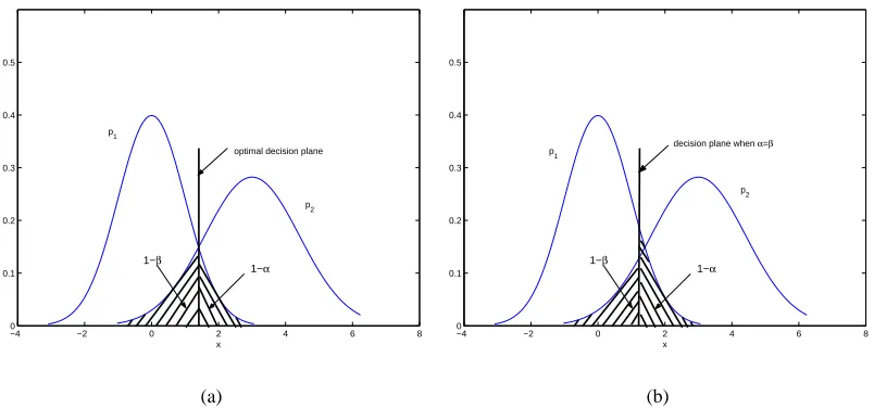
An analogy to illustrate the difference between MEMPM and MPM can be seen in the optimal thresholding problem. Figure 1 illustrates this analogy. To separate two classes of one-dimensional data with density functions as p1 and p2, respectively, the optimal thresholding is given by the decision plane in Figure 1(a) (assuming the prior probabilities for two classes of data are equal). This optimal thesholding corresponds to the point minimizing the error rate (1−α) + (1−β)or maximizing the accuracyα+β, which is exactly the intersection point of two density functions
(1−αrepresents the area of 135o-line filled region and 1−βrepresents the area of 45o-line filled region). On the other hand, the thresholding point to forceα=βis not necessarily the optimal point to separate these two classes.
−4 −2 0 2 4 6 8
0 0.1 0.2 0.3 0.4 0.5
x
1−α
1−β
p1
p2 optimal decision plane
(a)
−4 −2 0 2 4 6 8
0 0.1 0.2 0.3 0.4 0.5
x
1−α
1−β
p1
p2 decision plane when α=β
(b)
Figure 1: An analogy to illustrate the difference between MEMPM and MPM with equal prior probabilities for two classes. The optimal decision plane corresponds to the intersection point, where the error(1−α)+(1−β)is minimized (or the accuracyα+βis maximized) as implied by MEMPM, rather than the one, whereαis equal toβas implied by MPM.
2.3 Special Case for Biased Classification
The above discussion only covers unbiased classification, which does not favor one class over the other class intentionally. However, another important type of pattern recognition tasks, namely bi-ased classification, arises very often in practice. In this scenario, one class is usually more important than the other class. Thus a bias should be imposed towards the important class. Such typical ex-ample can be seen in the diagnosis of epidemical disease. Classifying a patient who is infected with a disease into the opposite class results in serious consequences. Thus in this problem, the classifi-cation accuracy should be biased towards the class with disease. In other words, we would prefer to diagnose the person without the disease to be the infected case rather than the other way round.
In the following we demonstrate that MEMPM contains a special case we call the Biased Mini-max Probability Machine for biased classification. We formulate this special case as
max
α,β,a6=0,b α s.t. inf
x∼(x,Σx)
Pr{aTx≥b} ≥α,
inf
y∼(y,Σy)
Pr{aTy≤b} ≥β0,
where β0 ∈[0, 1), a pre-specified constant, represents an acceptable accuracy level for the less important class y.
The above optimization utilizes a typical setting in biased classification, i.e., the accuracy for the important class (associated with x) should be as high as possible, if only the accuracy for the less important class (associated with y) maintains at an acceptable level specified by the lower boundβ0 (which can be set by users).
By quantitatively plugging a specified biasβ0 into classification and also by containing an ex-plicit accuracy boundα for the important class, BMPM provides a direct and elegant means for biased classification. Comparatively, to achieve a specified bias, traditional biased classifiers such as the Weighted Support Vector Machine (Osuna et al., 1997) and the Weighted k-Nearest Neighbor method (Maloof et al., 2003) usually adapt different costs for different classes. However, due to the difficulties in establishing quantitative connections between the costs and the accuracy,1for impos-ing a specified bias, these methods have to resort to trial and error procedure to attain suitable costs; these procedures are generally indirect and lack rigorous treatments.
2.4 Solving the MEMPM Optimization Problem
In this section, we will propose to solve the MEMPM optimization problem. As will be demon-strated shortly, the MEMPM optimization can be transformed to a one-dimensional line search problem. More specifically, the objective function of the line search problem is implicitly deter-mined by dealing with a BMPM problem. Therefore, solving the line search problem corresponds to solving a Sequential Biased Minimax Probability Machine (SBMPM) problem. Before we pro-ceed, we first introduce how to solve the BMPM optimization problem.
2.4.1 SOLVING THEBMPM OPTIMIZATIONPROBLEM
First, we borrow Lemma 1 from Lanckriet et al. (2002b).
Lemma 1 Given a6=0 and b, such that aTy≤b andβ∈[0,1), the condition
inf
y∼(y,Σy)
Pr{aTy≤b} ≥β,
holds if and only if b−aTy≥κ(β)p
aTΣ
ya withκ(β) =
q
β
1−β.
By using Lemma 1, we can transform the BMPM optimization problem as follows: max
α,a6=0,b α s.t.
−b+aTx≥κ(α)paTΣ
xa, (4)
b−aTy≥κ(β0)
q aTΣ
ya, (5)
whereκ(α) =q1−αα, κ(β0) =
q
β0
1−β0. (5) is directly obtained from (3) by using Lemma 1.
Simi-larly, by changing aTx≥b to aT(−x)≤ −b, (4) can be obtained from (2).
From (4) and (5), we get
aTy+κ(β0)
q aTΣ
ya≤b≤aTx−κ(α)
p aTΣ
xa.
If we eliminate b from this inequality, we obtain
aT(x−y)≥κ(α)paTΣ
xa+κ(β0)
q aTΣ
ya. (6)
We observe that the magnitude of a does not influence the solution of (6). Moreover, we can assume x6=y; otherwise, the minimax machine does not have a physical meaning. In this case, (6) may even have no solution for everyβ06=0, since the right hand side would always be positive provided that a6=0. Thus in the extreme case,αandβhave to be zero, implying that the worst-case classification accuracy is always zero.
Without loss of generality, we can set aT(x−y) =1. Thus the problem can further be changed to:
max
α,a6=0 α s.t.
1≥κ(α)paTΣ
xa+κ(β0)
q aTΣ
ya, (7)
aT(x−y) =1.
SinceΣxcan be assumed to be positive definite (otherwise, we can always add a small positive
amount to its diagonal elements and make it positive definite), from (7) we can obtain:
κ(α)≤ 1−κ(β0)
p aTΣ
ya
p aTΣ
Becauseκ(α)increases monotonically withα, maximizingαis equivalent to maximizingκ(α), which further leads to
max
a6=0
1−κ(β0)p aTΣ
ya
p aTΣ
xa
s.t. aT(x−y) =1.
This kind of optimization is called the Fractional Programming (FP) problem (Schaible, 1995). To elaborate further, this optimization is equivalent to solving the following fractional problem:
max
a6=0
f(a)
g(a) , (8)
subject to a∈A={a|aT(x−y) =1}, where f(a) =1−κ(β0)p aTΣ
ya,g(a) =
p aTΣ
xa.
Theorem 2 The Fractional Programming problem (8) associated with the BMPM optimization is a
pseudo-concave problem, whose every local optimum is the global optimum.
Proof It is easy to see that the domain A is a convex set onRn, and that f(a)and g(a)are differ-entiable on A. Moreover, sinceΣxandΣycan be both considered as positive definite matrices, f(a)
is a concave function on A and g(a)is a convex function on A. Then gf(a)(a) is a concave-convex FP problem. Hence it is a pseudoconcave problem (Schaible, 1995). Therefore, every local maximum is the global maximum (Schaible, 1995).
To handle this specific FP problem, many methods such as the parametric method (Schaible, 1995), the dual FP method (Schaible, 1977; Craven, 1988), and the concave FP method (Craven, 1978) can be used. A typical Conjugate Gradient method (Bertsekas, 1999) in solving this problem has a worst-case O(n3)time complexity. Adding the time cost to estimate x, y,Σx, andΣy, the total
cost for this method is O(n3+Nn2), where N is the number of data points. This complexity is in the same order as the linear Support Vector Machines (Sch¨olkopf and Smola, 2002) and the linear MPM (Lanckriet et al., 2002b).
In this paper, the Rosen gradient projection method (Bertsekas, 1999) is used to find the solution of this pseudo-concave FP problem, which is proved to converge to a local maximum with a worst-case linear convergence rate. Moreover, the local maximum will exactly be the global maximum in this problem.
2.4.2 SEQUENTIAL BMPM OPTIMIZATIONMETHOD FORMEMPM
We now turn to solving the MEMPM problem. Similar to Section 2.4.1, we can base Lemma 1 to transform the MEMPM optimization as follows:
max
α,β,a6=0,b θα+ (1−θ)β s.t.
−b+aTx≥κ(α)paTΣ
xa, (9)
b−aTy≥κ(β)
q aTΣ
Using an analysis similar to that in Section 2.4.1, we can further transform the above optimiza-tion to:
max
α,β,a6=0 θα+ (1−θ)β s.t. (11)
1≥κ(α)paTΣ
xa+κ(β)
q aTΣ
ya, (12)
aT(x−y) =1. (13)
In the following we provide a lemma to show that the MEMPM solution is attained on the boundary of the set formed by the constraints of (12) and (13).
Lemma 3 The maximum value ofθα+ (1−θ)βunder the constraints of (12) and (13) is achieved when the right hand side of (12) is strictly equal to 1.
Proof Assume the maximum is achieved when 1>κ(β)p aTΣ
ya+κ(α)
p aTΣ
xa. A new solution
constructed by increasingαorκ(α)a small positive amount,2and maintainingβ, a unchanged will satisfy the constraints and will be a better solution.
By applying Lemma 3, we can transform the optimization problem (11) under the constraints of (12) and (13) as follows:
max
β,a6=0
θκ2(α)
κ2(α) +1+ (1−θ)β s.t. (14)
aT(x−y) =1, (15)
whereκ(α) =1−κ(β)
√
aT∑
ya
√
aT∑
xa
.
In (14), if we fixβto a specific value within[0,1), the optimization is equivalent to maximizing
κ2(α)
κ2(α)+1 and further equivalent to maximizingκ(α), which is exactly the BMPM problem. We can
then update βaccording to some rules and repeat the whole process until an optimal βis found. This is also the so-called line search problem (Bertsekas, 1999). More precisely, if we denote the value of optimization as a function f(β), the above procedure corresponds to finding an optimalβ to maximize f(β). Instead of using an explicit function as in traditional line search problems, the value of the function here is implicitly given by a BMPM optimization procedure.
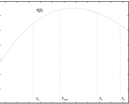
Many methods can be used to solve the line search problem. In this paper, we use the Quadratic Interpolation (QI) method (Bertsekas, 1999). As illustrated in Figure 2, QI finds the maximum point by updating a three-point pattern (β1, β2, β3) repeatedly. The new β denoted by βnew is given by the quadratic interpolation from the three-point pattern. Then a new three-point pattern is constructed byβnew and two ofβ1,β2,β3. This method can be shown to converge superlinearly to a local optimum point (Bertsekas, 1999). Moreover, as shown in Section 7, although MEMPM generally cannot guarantee its concavity, empirically it is often concave. Thus the local optimum will often be the global optimum in practice.
2. Sinceκ(α)increases monotonically withα, increasingαa small positive amount corresponds to increasingκ(α)a
f(β)
β1 βnew β2 β3
Figure 2: A three-point pattern and Quadratic Line search method. Aβnew is obtained and a new three-point pattern is constructed byβnewand two ofβ1,β2andβ3.
Until now, we do not mention how to calculate the intercept b. From Lemma 3, we can see that the inequalities (9) and (10) will become equalities at the maximum point(a∗,b∗). The optimal b will thus be obtained by
b∗=aT∗x−κ(α∗)
q aT
∗Σxa∗=aT∗y+κ(β∗) q
aT ∗Σya∗.
2.5 When Does the Worst-Case Bayes Optimal Hyperplane Become the True One?
As discussed, MEMPM derives the worst-case Bayes optimal hyperplane. Therefore, it is interesting to discover the conditions at which the worst-case optimal one changes to the true optimal one.
In the following we demonstrate two propositions. The first is that, when data are assumed to conform to some distributions, e.g., Gaussian distribution, the MEMPM framework leads to the Bayes optimal classifier; the second is that, when applied to high-dimensional classification tasks, the MEMPM model can be adapted to converge to the true Bayes optimal classifier under the Lyapunov condition.
To introduce the first proposition, we begin by assuming the data distribution as a Gaussian distribution.
Assuming x∼
N
(x,Σx)and y∼N
(y,Σy), (2) becomesinf
x∼N(x,Σx)
Pr{aTx≥b} = Prx∼N(x,Σx){a
Tx
≥b}
= Pr{
N
(0,1)≥ b−aTx p
aTΣ
xa
}
= 1−Φ( b−a
Tx p
aTΣ
xa )
= Φ(−b+a
Tx p
aTΣ
xa
whereΦ(z)is the cumulative distribution function for the standard normal Gaussian distribution: Φ(z) =Pr{
N
(0,1)≤z}=√12π
Z z
−∞exp(−s 2/2)ds. Due to the monotonic property ofΦ(z), we can further write (16) as
−b+aTx≥Φ−1(α)paTΣ
xa.
Constraint (3) can be reformulated in a similar form. The optimization (1) is thus changed to: max
α,β,a6=0,b θα+ (1−θ)β s.t.
−b+aTx≥Φ−1(α)p
aTΣ
xa, (17)
b−aTy≥Φ−1(β)
q aTΣ
ya. (18)
The above optimization is nearly the same as (1) subject to the constraints of (2) and (3) except that κ(α)is equal toΦ−1(α), instead ofq1−αα. Thus, it can similarly be solved based on the Sequential Biased Minimax Probability Machine method.
On the other hand, the Bayes optimal hyperplane corresponds to the one, aTz=b that minimizes the Bayes error:
min
a6=0,b θPrx∼N(x,Σx){a Tx
≤b}+ (1−θ)Pry∼N(y,Σy){a
Ty
≥b}.
The above is exactly the upper bound of θα+ (1−θ)β. From Lemma 3, we can know (17) and
(18) will eventually become equalities. Traced back to (16), the equalities imply that α and β will achieve their upper bounds respectively. Therefore, when Gaussianity is assumed for the data, MEMPM derives the optimal Bayes hyperplane.
We propose Proposition 4 to extend the above analysis to general distribution assumptions. Proposition 4 If the distribution of the normalized random variable a√Tx−aTx
aTΣ
xa
, denoted as
N S
, isindependent of a, minimizing the Bayes error bound in MEMPM exactly minimizes the true Bayes
error, provided thatΦ(z)is changed to Pr{
N S
(0,1)≤z}.Before presenting Proposition 6, we first introduce the central limit theorem under the Lyapunov condition (Chow and Teicher, 1997).
Theorem 5 Let xnbe a sequence of independent random variables defined on the same probability
space. Assume that xn has finite expected value µn and finite standard deviation σn. We define
s2
n=∑ni=1σ2i. Assume that the Lyapunov conditions are satisfied, namely, the third central moment
rn3=∑ni=1E(|xn−µn|3) is finite for every n, and that limn→∞rsnn =0. The sum Sn =x1+...+xn
converges towards a Gaussian distribution.
One interesting finding directly elicited from the above central limit theorem is that, if the com-ponent variable xiof a given n-dimensional random variable x satisfies the Lyapunov condition, the sum of weighted component variables xi, 1≤i≤n, namely, aTx tends towards a Gaussian distri-bution, as n grows.3 This shows that, under the Lyapunov condition, when the dimension n grows,
the hyperplane derived by MEMPM with the Gaussianity assumption tends towards the true Bayes optimal hyperplane. In this case, the MEMPM usingΦ−1(α), the inverse function of the normal cu-mulative distribution, instead ofq1−αα, will converge to the true Bayes optimal decision hyperplane in the high-dimensional space. We summarize the analysis in Proposition 6.
Proposition 6 If the component variable xi of a given n-dimensional random variable x satisfies
the Lyapunov condition, the MEMPM hyperplane derived by usingΦ−1(α), the inverse function of
the normal cumulative distribution, will converge to the true Bayes optimal one.
The underlying justifications in the above two propositions are rooted in the fact that the gen-eralized MPM is exclusively determined by the first and second moments. These two propositions emphasize the dominance of the first and second moments in representing data. More specifically, Proposition 4 hints that the distribution is only decided by up to the second moments. The Lyapunov condition in Proposition 6 also implies that the second order moment dominates the third order mo-ment in the long run. It is also noteworthy that, with a fixed mean and covariance, the distribution of Maximum Entropy Estimation is a Gaussian distribution (Keysers et al., 2002). This would once again suggest the usage ofΦ−1(α)in the high-dimensional space.
2.6 Geometrical Interpretation
In this section, we first provide a parametric solving method for BMPM. We then demonstrate that this parametric method enables a nice geometrical interpretation for both BMPM and MEMPM.
2.6.1 A PARAMETRICMETHOD FORBMPM
We present a parametric method to solve BMPM in the following. When compared with Gradient methods, this approach is relatively slow, but it need not calculate the gradient in each step and hence may avoid accumulated errors.
According to the parametric method, the fractional function can be iteratively optimized in two steps (Schaible, 1995):
Step 1: Find a by maximizing f(a)−λg(a)in the domain A, whereλ∈Ris the newly introduced parameter.
Step 2: Updateλby gf(a)(a).
The iteration of the above two steps will guarantee to converge to a local maximum, which is also the global maximum in our problem. In the following, we adopt a method to solve the maximization problem in Step 1. Replacing f(a)and g(a), we expand the optimization problem to:
max
a6=0 1−κ(β0)
q aTΣ
ya−λ
p aTΣ
xa s.t. aT(x−y) =1. (19)
Maximizing (19) is equivalent to minaκ(β0)
p aTΣ
ya+λ
p aTΣ
xa under the same constraint. By
writing a=a0+Fu, where a0= (x−y)/kx−yk2
2and F∈Rn×(n−1)is an orthogonal matrix whose columns span the subspace of vectors orthogonal to x−y, an equivalent form (a factor 12 over each term has been dropped) to remove the constraint can be obtained:
min
u,η>0,ξ>0η+ λ2
ηkΣx1/2(a0+Fu)k22+ξ+ κ(β0)2
whereη,ξ∈R. This optimization form is very similar to the one in the Minimax Probability Ma-chine (Lanckriet et al., 2002a) and can also be solved by using an iterative least-squares approach.
2.6.2 A GEOMETRICALINTERPRETATION FORBMPMANDMEMPM
The parametric method enables a nice geometrical interpretation of BMPM and MEMPM in a fash-ion similar to that of MPM in Lanckriet et al. (2002b). Again, we assume x6=y for the meaningful classification and assume thatΣxandΣyare positive definite for the purpose of simplicity.
By using the 2-norm definition of a vector z :kzk2=max{uTz :kuk2≤1}, we can express (19) as its dual form:
τ∗:=min
a6=0maxu,v λu
TΣ1/2
x a+κ(β0)vTΣy1/2a+τ(1−aT(x−y)): kuk2≤1,kvk2≤1. We change the order of the min and max operators and consider the min:
min
a6=0 λu
TΣ1/2
x a+κ(β0)vTΣy1/2a+τ(1−aT(x−y)) =
(
τ ifτx−λΣ1x/2u=τy+κ(β0)Σ1y/2v
−∞ otherwise .
Thus, the dual problem can further be changed to:
max
τ,u,v τ:kuk2≤1,kvk2≤1,τx−λΣ
1/2
x u=τy+κ(β0)Σ1y/2v.
By defining`:=1/τ, we rewrite the dual problem as
min
`,u,v `: x−λΣ
1/2
x u=y+κ(β0)Σ1y/2v,kuk2≤`,kvk2≤` . (20) When the optimum is attained, we have
τ∗=λkΣx1/2a∗k2+κ(β0)kΣ1y/2a∗k2=1/`∗.
We consider each side of (20) as an ellipsoid centered at the mean x and y and shaped by the weighted covariance matricesλΣxandκ(β0)Σyrespectively:
H
x(`) ={x=x+λΣx1/2u :kuk2≤`},H
y(`) ={y=y+κ(β0)Σy1/2v :kvk2≤`}.The above optimization involves finding a minimum`for which two ellipsoids intersect. For the optimum`, these two ellipsoids are tangential to each other. We further note that, according to Lemma 3, at the optimum,λ∗, which is maximized via a series of the above procedures, satisfies
1=λ∗kΣx1/2a∗k2+κ(β0)kΣ1y/2a∗k2=τ∗=1/`∗
⇒`∗=1.
grow with the same speed (with the same κ(α) and κ(β)). On the other hand, since MEMPM corresponds to solving a sequence of BMPMs, it similarly leads to a hyperplane tangential to two ellipsoids, which achieves to minimize the maximum of the worst-case Bayes error. Moreover, it is not necessarily attained in a balanced way as in MPM, i.e., two ellipsoids do not necessarily grow with the same speed and hence probably contain the unequal Mahalanobis distance from their corresponding centers. This is illustrated in Figure 3.
−6 −4 −2 0 2 4 6 8 10 12 14 16
−4 −2 0 2 4 6 8 10 12 14
o
o
Data: Class x depicted as +’s and Class y depicted as o’s
MPM BMPM MEMPM
K=1.28 K=2.32 K=2.77 K=2.77
K=3.54 K=5.35
Figure 3: The geometrical interpretation of MEMPM and BMPM. Finding the optimal BMPM hy-perplane corresponds to finding the decision plane (the black dashed line) tangential to an ellipsoid (the inner red dashed ellipsoid on the y side) , which is centered at y, shaped by the covariance Σy and whose Mahalanobis distance to y is exactly equal to κ(β0)
(κ(β0) =1.28 in this example). The worst-case accuracyα for x is determined by the Mahalanobis distanceκ(κ=5.35 in this example), at which, an ellipsoid (centered at x and shaped byΣx) is tangential to thatκ(β0)ellipsoid, i.e., the outer red dashed ellipsoid
3. Robust Version
In the above, the estimates of means and covariance matrices are assumed reliable. We now consider how the probabilistic framework in (1) changes in the face of variation of the means and covariance matrices:
max
α,β,a6=0,b θα+ (1−θ)β s.t. inf
x∼(¯x,Σx)
Pr{aTx≥b} ≥α,∀(¯x,Σx)∈
X
,inf
y∼(¯y,Σy)
Pr{aTy≤b} ≥β,∀(¯y,Σy)∈
Y
,where
X
andY
are the sets of means and covariance matrices and are the subsets ofR×P
+n , where
P
+n is the set of n×n symmetric positive semidefinite matrices.
Motivated by the tractability of the problem and from a statistical viewpoint, a specific setting of
X
andY
has been proposed in Lanckriet et al. (2002b). However, these authors consider the same variations of the means for two classes, which is easy to handle but less general. Now, considering the unequal treatment of each class, we propose the following setting, which is in a more general and complete form:X
=(¯x,Σx)|(¯x−¯x0)Σx−1(¯x−¯x0)≤ν2x,kΣx−Σx0kF≤ρx ,
Y
=(¯y,Σy)|(¯y−¯y0)Σy−1(¯y−¯y0)≤ν2y,kΣy−Σy0kF≤ρy ,
where ¯x0,Σ0xare the “nominal” mean and covariance matrices obtained through estimation. Param-etersνx,νy,ρx, andρy are positive constants. The matrix norm is defined as the Frobenius norm:
kMk2F=Tr(MTM).
With the equality assumption for the variations of the means for two classes, the parametersνx
andνyare required equal in Lanckriet et al. (2002b). This enables the direct usage of the MPM
op-timization in its robust version. However, the assumption may not be valid in real cases. Moreover, in MEMPM, the assumption is also unnecessary and inappropriate. This will be demonstrated later in the experiment.
By applying the results from Lanckriet et al. (2002b), we obtain the robust MEMPM as max
α,β,a6=0,b θα+ (1−θ)β s.t.
−b+aT¯x0≥(κ(α) +νx)
q aT(Σ 0
x +ρxIn)a,
b−aT¯y0≥(κ(β) +νy)
q aT(Σ 0
y +ρyIn)a. Analogously, we transform the above optimization problem to
max
α,β,a6=0θ
κ2 r(α) 1+κ2
r(α)
+ (1−θ)β s.t. aT(¯x0−¯y0) =1,
where κr(α) =max
1−(κ(β)+νy)√aT(Σy0+ρyIn)a
√
aT(Σ0
x +ρxIn)a − νx,0
and thus can be solved by the SBMPM method. The optimal b is therefore calculated by
b∗ = a∗T¯x0−(κ(α∗) +νx)
q
a∗T(Σ 0
x +ρxIn)a∗
= a∗T¯y0+ (κ(β∗) +νy)
q
a∗T(Σ 0
Remarks. Interestingly, if MPM is treated with unequal robust parametersνxandνy, it leads
to solving an optimization similar to MEMPM, sinceκ(α) +νxwill not be equal toκ(α) +νy. In
addition, similar to the robust MPM, when applied in practice, the specific values ofνx,νy,ρx, and
ρycan be provided based on the central limit theorem or the resampling method.
4. Kernelization
We note that, in the above, the classifier derived from MEMPM is given in a linear configuration. In order to handle nonlinear classification problems, in this section, we seek to use the kernelization trick (Sch¨olkopf and Smola, 2002) to map the n-dimensional data points into a high-dimensional feature space Rf, where a linear classifier corresponds to a nonlinear hyperplane in the original space.
Since the optimization of MEMPM corresponds to a sequence of BMPM optimization problems, this model will naturally inherit the kernelization ability of BMPM. We thus in the following mainly address the kernelization of BMPM.
Assuming training data points are represented by{xi}Ni=x1and{yj} Ny
j=1for the class x and class y, respectively, the kernel mapping can be formulated as
x→ϕ(x)∼(ϕ(x),Σϕ(x)),
y→ϕ(y)∼(ϕ(y),Σϕ(y)),
whereϕ:Rn→Rf is a mapping function. The corresponding linear classifier inRf is aTϕ(z) =b,
where a,ϕ(z)∈Rf, and b∈R. Similarly, the transformed FP optimization in BMPM can be written as
max
a
1−κ(β0)qaTΣ
ϕ(y)a q
aTΣ
ϕ(x)a
s.t. aT(ϕ(x)−ϕ(y)) =1. (21)
However, to make the kernel work, we need to represent the final decision hyperplane and the optimization in a kernel form, K(z1,z2) =ϕ(z1)Tϕ(z2), namely an inner product form of the mapping data points.
4.1 Kernelization Theory for BMPM
In the following, we demonstrate that, although BMPM possesses a significantly different optimiza-tion form from MPM, the kernelizaoptimiza-tion theory proposed in Lanckriet et al. (2002b) is still viable, provided that suitable estimates for means and covariance matrices are applied therein.
We first state a theory similar to Corollary 5 of Lanckriet et al. (2002b) and prove its validity in BMPM.
Corollary 7 If the estimates of means and covariance matrices are given in BMPM as ϕ(x) =
Nx
∑
i=1
λiϕ(xi), ϕ(y) = Ny
∑
j=1
Σϕ(x)=ρxIn+ Nx
∑
i=1
Λi(ϕ(xi)−ϕ(x))(ϕ(xi)−ϕ(x))T ,
Σϕ(y)=ρyIn+ Ny
∑
j=1
Ωj(ϕ(yj)−ϕ(y))(ϕ(yj)−ϕ(y))T ,
where In is the identity matrix of dimension n, then the optimal a in problem (21) lies in the space
spanned by the training points.
Proof Similar to Lanckriet et al. (2002b), we write a=ap+ad, where apis the projection of a in the vector space spanned by all the training data points and ad is the orthogonal component to this span space. It can be easily verified that (21) changes to maximize the following:
1−κ(β0)
q aT
p∑ Nx
i=1Λi(ϕ(xi)−ϕ(x))(ϕ(xi)−ϕ(x))Twp+ρx(aTpap+wTdad) q
aT p∑
Ny
j=1Ωj(ϕ(yj)−ϕ(y))(ϕ(yj)−ϕ(y))Tap+ρy(aTpap+aTdad) subject to the constraints of aTp(ϕ(x)−ϕ(y)) =1.
Since we intend to maximize the fractional form and both the denominator and the numerator are positive, the denominator needs to be as small as possible and the numerator needs to be as large as possible. This would finally lead to ad=0. In other words, the optimal a lies in the vector space spanned by all the training data points. Note that the introduction of ρx and ρy enables a direct
application of the robust estimates in the kernelization.
According to Corollary 7, if appropriate estimates of means and covariance matrices are applied, the optimal a can be written as the linear combination of training points. In particular, if we obtain the means and covariance matrices as the plug-in estimates, i.e.,
ϕ(x) = 1
Nx
Nx
∑
i=1 ϕ(xi),
ϕ(y) = 1
Ny
Ny
∑
j=1 ϕ(yj),
Σϕ(x)=N1 x
Nx
∑
i=1
(ϕ(xi)−ϕ(x))(ϕ(xi)−ϕ(x))T,
Σϕ(y)= 1
Ny
Ny
∑
j=1
(ϕ(yj)−ϕ(y))(ϕ(yj)−ϕ(y))T ,
we can write a as
a=
Nx
∑
i=1
µiϕ(xi) + Ny
∑
j=1
υjϕ(yj), (22)
where the coefficients µi,υj∈R,i=1, . . . ,Nx, j=1, . . . ,Ny.
Kernelization Theorem of BMPM The optimal decision hyperplane of the problem (21) involves
solving the Fractional Programming problem
κ(α∗) =max
w6=0
1−κ(β0)q 1 Nyw
TK˜T
yK˜yw
q 1 Nxw
TK˜T
xK˜xw
s.t. wT(˜kx−˜ky) =1. (23)
The intercept b is calculated as
b∗=wT∗˜kx−κ(α∗)
r 1
Nx
wT
∗K˜TxK˜xw∗=wT∗˜ky+κ(β0)
s 1
Ny
wT
∗K˜TyK˜yw∗,
whereκ(α∗)is obtained when (23) attains its optimum(w∗,b∗). For the robust version of BMPM,
we can incorporate the variations of the means and covariances by conducting the following re-placements:
1
Nx
wT∗K˜TxK˜xw∗→wT∗( 1
Nx
˜
KTxK˜x+ρxK)w∗, 1
Ny
wT∗K˜TyK˜yw∗→wT∗( 1
Ny
˜
KTyK˜y+ρyK)w∗, κ(β0)→κ(β0) +µy,
κ(α∗)→κ(α∗) +µx.
The optimal decision hyperplane can be represented as a linear form in the kernel space
f(z) =
Nx
∑
i=1
w∗iK(z,xi) + Ny
∑
i=1
w∗Nx+iK(z,yi)−b∗.
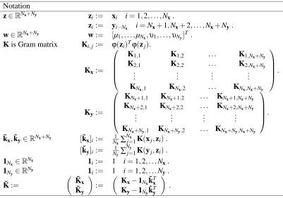
The notation in the above are defined in Table 1.
5. Experiments
In this section, we first evaluate our model on a synthetic data set. Then we compare the performance of MEMPM with that of MPM, on six real world benchmark data sets. To demonstrate that BMPM is ideal for imposing a specified bias in classification, we also implement it on the Heart-disease data set. The means and covariance matrices for two classes are obtained directly from the training data sets by plug-in estimations. The prior probabilityθis given by the proportion of x data in the training set.
5.1 Model Illustration on a Synthetic Data Set
To verify that the MEMPM model achieves the minimum Bayes error rate in the Gaussian dis-tribution, we synthetically generate two classes of two-dimensional Gaussian data. As plotted in Figure 4(a), data associated with the class x are generated with the mean x as[3,0]T and the covari-ance matrixΣxas[4, 0; 0,1], while data associated with the class y are generated with the mean y
as[−1,0]T and the covariance matrixΣ
Notation
z∈RNx+Ny z
i:= xi i=1,2, . . . ,Nx.
zi:= yi−Nx i=Nx+1,Nx+2, . . . ,Nx+Ny.
w∈RNx+Ny w := [µ
1, . . . ,µNx,υ1, . . . ,υNy]
T.
K is Gram matrix Ki,j:= ϕ(zi)Tϕ(zj).
Kx:=
K1,1 K1,2 . . . K1,Nx+Ny
K2,1 K2,2 . . . K2,Nx+Ny
..
. ... ... ...
KNx,1 KNx,2 . . . KNx,Nx+Ny
.
Ky:=
KNx+1,1 KNx+1,2 . . . KNx+1,Nx+Ny
KNx+2,1 KNx+2,2 . . . KNx+2,Nx+Ny
..
. ... ... ...
KNx+Ny,1 KNx+Ny,2 . . . KNx+Ny,Nx+Ny
.
˜kx,˜ky∈RNx+Ny [˜kx]i:= N1x∑Nj=x1K(xj,zi).
[˜ky]i:= N1y∑ Ny
j=1K(yj,zi). 1Nx ∈R
Nx 1
i:= 1 i=1,2, . . .Nx.
1Ny ∈R
Ny 1
i:= 1 i=1,2, . . .Ny.
˜ K :=
˜ Kx ˜ Ky :=
Kx−1Nx˜k
T
x
Ky−1Ny˜k
T
y
.
Table 1: Notation used in Kernelization Theorem of BMPM
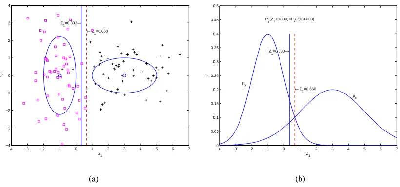
given by MPM is plotted as the solid blue line and the solved decision hyperplane Z1=0.660 given by MEMPM is plotted as the dashed red line. From the geometrical interpretation, both hyperplanes should be perpendicular to the Z1axis.
As shown in Figure 4(b), the MEMPM hyperplane exactly represents the optimal thresholding under the distributions of the first dimension for two classes of data, i.e., the intersection point of two density functions. On the other hand, we find that, the MPM hyperplane exactly corresponds to the thresholding point with the same error rate for two classes of data, since the cumulative distributions
Px(Z1<0.333)and Py(Z1>0.333)are exactly the same.
5.2 Evaluations on Benchmark Data Sets
We next evaluate our algorithm on six benchmark data sets. Data for Twonorm problem were generated according to Breiman (1997). The remaining five data sets (Breast, Ionosphere, Pima, Heart-disease, and Vote) were obtained from the UCI machine learning repository (Blake and Merz, 1998). Since handling the missing attribute values is out of the scope of this paper, we simply remove instances with missing attribute values in these data sets.
−4 −3 −2 −1 0 1 2 3 4 5 6 7 −4
−3 −2 −1 0 1 2 3 4
Z1
Z2
← Z1=0.660 Z1=0.333→
(a)
−4 −3 −2 −1 0 1 2 3 4 5 6 7
0 0.05 0.1 0.15 0.2 0.25 0.3 0.35 0.4 0.45 0.5
Z1
p
← Z1=0.660 Z1=0.333→
Py(Z1<0.333)=Px(Z1>0.333)
py
px
(b)
Figure 4: An experiment on a synthetic data set. The decision hyperplane derived from MEMPM (the dashed red line) exactly corresponds to the optimal thresholding point, i.e., the inter-section point, while the decision hyperplane given by MPM (the solid blue line) corre-sponds to the point in which the error rates for the two classes of data are equal.
From the results, we can see that our MEMPM demonstrates better performance than MPM in both the linear setting and Gaussian kernel setting. Moreover, in these benchmark data sets, the MEMPM hyperplanes are obtained with significantly unequal αandβ except in Twonorm. This further confirms the validity of our proposition, i.e., the optimal minimax machine is not certain to achieve the same worst-case accuracies for two classes. Twonorm is not an exception to this. The two classes of data in Twonorm are generated under the multivariate normal distributions with the same covariance matrices. In this special case, the intersection point of two density functions will exactly represent the optimal thresholding point and the one with the same error rate for each class as well. Another important finding is that the accuracy bounds, namelyθα+ (1−θ)βin MEMPM and αin MPM, are all increased in the Gaussian kernel setting when compared with those in the linear setting. This shows the advantage of the kernelized probability machine over the linear probability machine.
In addition, to show the relationship between the bounds and the test set accuracies (TSA) clearly, we plot them in Figure 5. As observed, the test set accuracies including TSAx (for class
x), TSAy(for the class y), and the overall accuracies TSA are all greater than their corresponding
accuracy bounds in both MPM and MEMPM. This demonstrates how the accuracy bound can serve as the performance indicator on future data. It is also observed that the overall worst-case accuracies θα+ (1−θ)βin MEMPM are greater thanαin MPM both in the linear and Gaussian setting. This again demonstrates the superiority of MEMPM to MPM.
Twonorm0 Breast Iono Pima Heart−disease Vote 10 20 30 40 50 60 70 80 90 100 Percentage
α’s and TSAx’s in the linear kernel
α
TSAx
(a)
Twonorm0 Breast Iono Pima Heart−disease Vote 10 20 30 40 50 60 70 80 90 100 Percentage
α’s and TSAx’s in the Gaussian kernel
α
TSAx
(b)
Twonorm0 Breast Iono Pima Heart−disease Vote 10 20 30 40 50 60 70 80 90 100 Percentage
β’s and TSAy’s in the linear kernel
β
TSAy
(c)
Twonorm0 Breast Iono Pima Heart−disease Vote 10 20 30 40 50 60 70 80 90 100 Percentage
β’s and TSAy’s in the Gaussian kernel
β
TSAy
(d)
Twonorm0 Breast Iono Pima Heart−disease Vote 10 20 30 40 50 60 70 80 90 100 Percentage
Bounds and TSA’s for MEMPM and MPM in the linear kernel
θα+(1−θ)β
TSA:MEMPM
α
TSA:MPM
(e)
Twonorm20 Breast Iono Pima Heart−disease Vote 30 40 50 60 70 80 90 100 Percentage
Bounds and TSA’s for MEMPM and MPM in the Gaussian kernel
θα+(1−θ)β
TSA:MEMPM
α
TSA:MPM
(f)
Figure 5: Bounds and test set accuracies. The test accuracies including TSAx(for the class x), TSAy
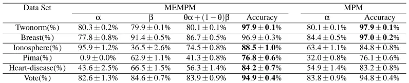
Data Set MEMPM MPM
α β θα+ (1−θ)β Accuracy α Accuracy
Twonorm(%) 80.3±0.2% 79.9±0.1% 80.1±0.1% 97.9±0.1% 80.1±0.1% 97.9±0.1%
Breast(%) 77.8±0.8% 91.4±0.5% 86.7±0.5% 96.9±0.3% 84.4±0.5% 97.0±0.2%
Ionosphere(%) 95.9±1.2% 36.5±2.6% 74.5±0.8% 88.5±1.0% 63.4±1.1% 84.8±0.8% Pima(%) 0.9±0.0% 62.9±1.1% 41.3±0.8% 76.8±0.6% 32.0±0.8% 76.1±0.6% Heart-disease(%) 43.6±2.5% 66.5±1.5% 56.3±1.4% 84.2±0.7% 54.9±1.4% 83.2±0.8% Vote(%) 82.6±1.3% 84.6±0.7% 83.9±0.9% 94.9±0.4% 83.8±0.9% 94.8±0.4% Table 2: Lower boundα,β, and test accuracy compared to MPM in the linear setting.
Data Set MEMPM MPM
α β θα+ (1−θ)β Accuracy α Accuracy
Twonorm(%) 91.7±0.2% 91.7±0.2% 91.7±0.2% 97.9±0.1% 91.7±0.2% 97.9±0.1%
Breast(%) 88.4±0.6% 90.7±0.4% 89.9±0.4% 96.9±0.2% 89.9±0.4% 96.9±0.3%
Ionosphere(%) 94.2±0.8% 80.9±3.0% 89.4±0.8% 93.8±0.4% 89.0±0.8% 92.2±0.4% Pima(%) 2.6±0.1% 62.3±1.6% 41.4±1.1% 77.0±0.7% 32.1±1.0% 76.2±0.6% Heart-disease(%) 47.1±2.2% 66.6±1.4% 58.0±1.5% 83.9±0.9% 57.4±1.6% 83.1±1.0% Vote(%) 85.1±1.3% 84.3±0.7% 84.7±0.8% 94.7±0.5% 84.4±0.8% 94.6±0.4% Table 3: Lower boundα,β, and test accuracy compared to MPM with the Gaussian kernel.
[1 0; 0 3], while y data are sampled from another Gaussian distribution with the mean as [−3,0]T and the covariance as[3 0; 0 1]. We randomly select 10 points of each class for training and leave the remaining points for test from the above synthetic data set. We present the result below.
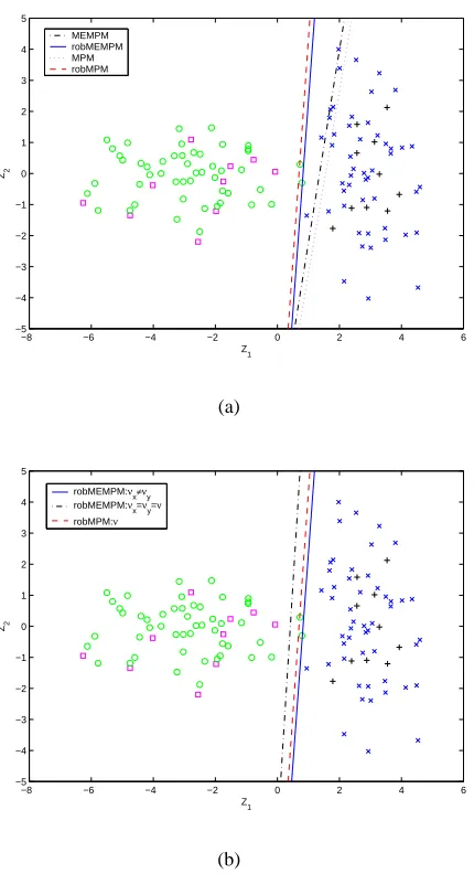
First, we calculate the corresponding means, ¯x0and ¯y0and covariance matrices,Σx0andΣy0and plug them into the linear MPM and the linear MEMPM. We obtain the MPM decision line (magenta dotted line) with a lower bound (assuming the Gaussian distribution) being 99.1% and the MEMPM decision line (black dash-dot line) with a lower bound of 99.7%. However, for the test set, we obtain the accuracies of only 93.0% for MPM and 97.0% for MEMPM (see Figure 6(a)). This obviously violates the lower bound.
Based on our knowledge of the real means and covariance matrices in this example, we set the parameters as
νx=
q
(¯x−¯x0)TΣ −1
x (¯x−¯x0) =0.046,νy=
q
(¯y−¯y0)TΣ−1
y (¯y−¯y0) =0.496,
ν=max(νx,νy), ρx=kΣx−Σx0kF =1.561, ρy=kΣy−Σy0kF =0.972.
We then train the robust linear MPM and the robust linear MEMPM by these parameters and obtain the robust MPM decision line (red dashed line), and the robust MEMPM decision line (blue solid line), as seen in Figure 6(a). The lower bounds decrease to 87.3% for MPM and 93.2% for MEMPM respectively, but the test accuracies increase to 98.0% for MPM and 100.0% for MEMPM. Obviously, the lower bounds accord with the test accuracies.
Note that in the above, the robust MEMPM also achieves better performance than the robust MPM. Moreover,νx andνy are not necessarily the same. To see the result of MEMPM when νx
andνy are forced to be the same, we train the robust MEMPM again by setting the parameters as
νx=νy=νas used in MPM. We obtain the corresponding decision line (black dash-dot line) as
seen in Figure 6(b). The lower bound decreases to 91.0% and the test accuracy decreases to 98.0%. The above example indicates how the robust MEMPM clearly improves on the standard MEMPM when a bias is incorporated by inaccurate plug-in estimates and also validates thatνx need not be
−8 −6 −4 −2 0 2 4 6 −5
−4 −3 −2 −1 0 1 2 3 4 5
Z1
Z2
MEMPM robMEMPM MPM robMPM
(a)
−8 −6 −4 −2 0 2 4 6
−5 −4 −3 −2 −1 0 1 2 3 4 5
Z
1
Z2
robMEMPM:νx≠νy
robMEMPM:νx=νy=ν
robMPM:ν
(b)
5.3 Evaluations of BMPM on the Heart-Disease Data Set
To demonstrate the advantages of the BMPM model in dealing with biased classification, we imple-ment BMPM on the Heart-disease data set, where a different treatimple-ment for different classes is nec-essary. The x class is associated with subjects with heart disease, whereas the y class corresponds to subjects without heart disease. Obviously, a bias should be considered for x, since misclassification of an x case into the opposite class would delay the therapy and may have a higher risk than the other way round. Similarly, we randomly partition data into 90% training and 10% test sets. Also, the width parameter (σ) for the Gaussian kernel is obtained via cross validations over 50 random partitions of the training set. We repeat the above procedures 50 times and report the average results. By intentionally varyingβ0 from 0 to 1, we obtain a series of test accuracies, including the x accuracy, TSAx, the y accuracy TSAy for both the linear and Gaussian kernel. For simplicity, we
denote the x accuracy in the linear setting as TSAx(L), while others are similarly defined.
The results are summarized in Figure 7. Four observations are worth highlighting. First, in both linear and Gaussian kernel settings, the smallerβ0 is, the higher the test accuracy for x becomes. This indicates that a bias can indeed be embedded in the classification boundary for the important class x by specifying a relatively smallerβ0. In comparison, MPM forces an equal treatment on each class and thus is not suitable for biased classification. Second, the test accuracies for y and x are strictly lower bounded byβ0 andα. This shows how a bias can be quantitatively, directly, and rigorously imposed towards the important class x. Note that again, for other weight-adapting based biased classifiers, the weights themselves lack accurate interpretations and thus cannot rigorously impose a specified bias, i.e., they would try different weights for a specified bias. Third, when given a prescribedβ0, the test accuracy for x and its worst-case accuracyαin the Gaussian kernel setting are both greater than the corresponding accuracies in the linear setting. Once again, this demonstrates the power of the kernelization. Fourth, we note that β0 actually contains an upper bound, which is around 90% for the linear BMPM in this data set. This is reasonable. Observed from (7), the maximumβ0, denoted asβ0m, is decided by settingα=0, i.e.,
κ(β0m) =max
a6=0
1 p
aTΣ
ya
s.t. aT(x−y) =1.
It is interesting to note that when β0 is set to zero, the test accuracies for y in the linear and Gaussian settings are both around 50% (see Figure 7(b)). This seeming “irrationality” is actually reasonable. We will discuss this in the next section.
6. How Tight Is the Bound?
A natural question for MEMPM is, how tight is the worst-case bound? In this section, we present a theoretical analysis in addressing this problem.
We begin with a lemma proposed in Popescu and Bertsimas (2001). sup
y∼(y,Σy)
Pr{y∈
S
}= 11+d2, with d 2=inf
y∈S(y−y)
TΣ−1
y (y−y), (24)
where
S
denotes a convex set.If we define
S
={aTy≥b}, the above lemma is changed to: supy∼{y,Σy}
Pr{aTy≥b}= 1
1+d2, with d
2= inf
aTy≥b(y−y)
TΣ−1
0 10 20 30 40 50 60 70 80 90 100 0
10 20 30 40 50 60 70 80 90 100
β(%)
α(L)
α(G)
TSAx(G) TSAx(L)
(a)
0 10 20 30 40 50 60 70 80 90 100
0 10 20 30 40 50 60 70 80 90 100
β(%)
TSAy(L)
TSAy(G)
β
(b)
Figure 7: Bounds and real accuracies. Withβ0 varying from 0 to 1, the real accuracies are lower bounded by the worst-case accuracies. In addition,α(G) is aboveα(L), which shows the power of the kernelization.
By reference to (3), for a given hyperplane{a,b}, we can easily obtain that β= d
2
1+d2 . (25)
Moreover, in Lanckriet et al. (2002b), a simple closed-form expression for the minimum dis-tance d is derived:
d2= inf
aTy≥b(y−y)
TΣ−1
y (y−y) =
max((b−aTy),0)2 aTΣ
ya
. (26)
It is easy to see that when the decision hyperplane{a,b}passes the center y, d would be equal to 0 and the worst-case accuracyβwould be 0 according to (25).
However, if we consider the Gaussian data (which we assume as y data) in Figure 8(a), a vertical line approximating y would achieve about 50% test accuracy. The large gap between the worst-case accuracy and the real test accuracy seems strange. In the following, we construct an example of one-dimensional data to show the inner rationality of this observation. We attempt to provide the worst-case distribution containing the given mean and covariance, while a hyperplane passing its mean achieves a real test accuracy of zero.
Consider one-dimensional data y consisting of N−1 observations with values as m and one single observation with the value asσ√N+m. If we calculate the mean and the covariance, we
obtain:
y=m+√σ
N ,
Σy=
N−1
N σ
When N goes to infinity, the above one-dimensional data have the mean as m and the covariance as σ. In this extreme case, a hyperplane passing the mean will achieve a zero test accuracy, which is exactly the worst-case accuracy given the fixed mean and covariance as m andσrespectively. This example demonstrates the inner rationality of the minimax probability machines.
−8 −6 −4 −2 0 2 4 6 8 −8
−6 −4 −2 0 2 4 6 8
Z1
Z2
aTy > b
aTy < b aTy = b
(a)
−8 −6 −4 −2 0 2 4 6 8 −8
−6 −4 −2 0 2 4 6 8
Z1
Z2
aTy < b aTy > b
aTy = b
(b)
−8 −6 −4 −2 0 2 4 6 8 −8
−6 −4 −2 0 2 4 6 8
Z1
Z2
aTy < b aTy > b
aTy = b
(c)
Figure 8: Three two-dimensional data sets with the same means and covariances but with different skewness. The worst-case accuracy bound of (a) is tighter than that of (b) and looser than that of (c).
To further examine the tightness of the worst-case bound in Figure 8(a), we varyβfrom 0 to 1 and plot againstβthe real test accuracy that a vertical line classifies the y data by using (25). Note that the real accuracy can be calculated asΦ(z≤d). This curve is plotted in Figure 9.
Observed from Figure 9, the smaller the worst-case accuracy is, the looser it is. On the other hand, if we skew the y data towards the left side, while simultaneously maintaining the mean and covariance unchanged (see Figure 8(b)), an even bigger gap will be generated when β is small; similarly, if we skew the data towards the right side (see Figure 8(c)), a tighter accuracy bound will be expected. This finding means that adopting up to the second order moments only may not achieve a satisfactory bound. In other words, for a tighter bound, higher order moments such as skewness may need to be considered. This problem of estimating a probability bound based on moments is presented as the(n,k,Ω)-bound problem, which means “finding the tightest bound for an n-dimensional variable in the setΩbased on up to the k-th moments.” Unfortunately, as proved in Popescu and Bertsimas (2001), it is NP-hard for(n,k,Rn)-bound problems with k≥3. Thus tightening the bound by simply scaling up the moment order may be intractable in this sense. We may have to exploit other statistical techniques to achieve this goal. This certainly deserves a closer examination in the future.
7. On the Concavity of MEMPM
0 0.1 0.2 0.3 0.4 0.5 0.6 0.7 0.8 0.9 1 0
0.1 0.2 0.3 0.4 0.5 0.6 0.7 0.8 0.9 1
Worst−case accuracy β
Real test accuracy
Figure 9: Theoretical comparison between the worst-case accuracy and the real test accuracy for the Gaussian data in Figure 8(a).
MEMPM model can be solved successfully by standard optimization methods, e.g., the linear search method proposed in this paper.
We first present a lemma for the BMPM model.
Lemma 8 The optimal solution for BMPM is a strictly and monotonically decreasing function with
respect toβ0.
Proof Let the corresponding optimal worst-case accuracies on x beα1andα2respectively, when β01andβ02are set to the acceptable accuracy levels for y in BMPM. We will prove that ifβ01>β02, thenα1<α2.
This can be proved by considering the contrary case, i.e., we assumeα1≥α2. From the problem definition of BMPM, we have:
α1≥α2=⇒κ(α1)≥κ(α2)
=⇒ 1−κ(β01)
p
a1TΣya1
p
a1TΣxa1
≥ 1−κ(β02)
p
a2TΣya2
p
a2TΣxa2
, (27)
where a1 and a2 are the corresponding optimal solutions that maximizeκ(α1) andκ(α2) respec-tively, whenβ01andβ02are specified.
Fromβ01>β02and (27), we have 1−κ(β02)p
a1TΣya1
p
a1TΣxa1
>1−κ(β01)
p
a1TΣya1
p
a1TΣxa1
≥1−κ(β02)
p
a2TΣya2
p
a2TΣxa2
. (28)
On the other hand, since a2is the optimal solution of maxa
1−κ(β02)√aTΣya
√
aTΣ
xa
, we have:
1−κ(β02)p
a2TΣya2
p
a2TΣxa2
≥1−κ(β02)
p
a1TΣya1
p

![Figure 4(a), data associated with the class x are generated with the mean x as [3,0] and the covari-ance matrix Σx as [4, 0;0, 1], while data associated with the class y are generated with the mean yas10T and the covariance matrix Σ as1 0;0 5](https://thumb-us.123doks.com/thumbv2/123dok_us/9842342.1970637/17.612.108.467.142.253/figure-associated-generated-covari-associated-generated-covariance-matrix.webp)