Gaussian Processes for Ordinal Regression

Gaussian Processes for Ordinal Regression

Wei Chu [email protected]

Zoubin Ghahramani [email protected]

Gatsby Computational Neuroscience Unit University College London

London, WC1N 3AR, UK

Editor: Christopher K. I. Williams

Abstract

We present a probabilistic kernel approach to ordinal regression based on Gaussian processes. A threshold model that generalizes the probit function is used as the likelihood function for ordinal variables. Two inference techniques, based on the Laplace approximation and the expectation prop-agation algorithm respectively, are derived for hyperparameter learning and model selection. We compare these two Gaussian process approaches with a previous ordinal regression method based on support vector machines on some benchmark and real-world data sets, including applications of ordinal regression to collaborative filtering and gene expression analysis. Experimental results on these data sets verify the usefulness of our approach.

Keywords: Gaussian processes, ordinal regression, approximate Bayesian inference, collaborative filtering, gene expression analysis, feature selection

1. Introduction

Practical applications of supervised learning frequently involve situations exhibiting an order among the different categories, e.g. a teacher always rates his/her students by giving grades on their overall performance. In contrast to metric regression problems, the grades are usually discrete and finite. These grades are also different from the class labels in classification problems due to the existence of ranking information. For example, grade labels have the ordering F <D<C<B<A. This is a learning task of predicting variables of ordinal scale, a setting bridging between metric regression and classification referred to as ranking learning or ordinal regression.

or-dinal regression and the numerical results they presented shows a significant improvement on the performance compared with the on-line algorithm proposed by Crammer and Singer (2002).

In the statistics literature, most of the approaches are based on generalized linear models (Mc-Cullagh and Nelder, 1983). The cumulative model (Mc(Mc-Cullagh, 1980) is well-known in classical statistical approaches for ordinal regression, in which they rely on a specific distributional assump-tion on the unobservable latent variables and a stochastic ordering of the input space. Johnson and Albert (1999) described Bayesian inference on parametric models for ordinal data using sampling techniques. Tutz (2003) presented a general framework for semiparametric models that extends generalized additive models (Hastie and Tibshirani, 1990) by incorporating nonparametric parts. The nonparametric components of the regression model are fitted by maximizing penalized log likelihood, and model selection is carried out using AIC.

Gaussian processes (O’Hagan, 1978; Neal, 1997) have provided a promising non-parametric Bayesian approach to metric regression (Williams and Rasmussen, 1996) and classification prob-lems (Williams and Barber, 1998). The important advantage of Gaussian process models (GPs) over other non-Bayesian models is the explicit probabilistic formulation. This not only provides prob-abilistic predictions but also gives the ability to infer model parameters such as those that control the kernel shape and the noise level. The GPs are also different from the semiparametric approach of Tutz (2003) in several ways. First, the additive models (Fahrmeir and Tutz, 2001) are defined by functions in each input dimension, whereas the GPs can have more general non-additive covariance functions; second, the kernel trick allows to use infinite basis function expansions; third, the GPs perform Bayesian inference in the space of the latent functions.

In this paper, we present a probabilistic kernel approach to ordinal regression in Gaussian pro-cesses. We impose a Gaussian process prior distribution on the latent functions, and employ an appropriate likelihood function for ordinal variables which can be regarded as a generalization of the probit function. Two Bayesian inference techniques are applied to implement model adapta-tion by using the Laplace approximaadapta-tion (MacKay, 1992) and the expectaadapta-tion propagaadapta-tion (Minka, 2001) respectively. Comparisons of the generalization performance against the support vector ap-proach (Shashua and Levin, 2003) on some benchmark and real-world data sets, such as movie ranking and gene expression analysis, verify the usefulness of this approach.

The paper is organized as follows: in Section 2, we describe the Bayesian framework in Gaus-sian processes for ordinal regression; in Section 3, we discuss the BayeGaus-sian techniques for hyperpa-rameter inference; in Section 4, we present the predictive distribution for probabilistic prediction; in Section 5, we give some extensive discussion on these techniques; in Section 6, we report the results of numerical experiments on some benchmark and real-world data sets; we conclude this paper in Section 7.

2. Bayesian Framework

Consider a data set composed of n samples. Each of the samples is a pair of input vector xi∈

R

d

and the corresponding target yi∈

Y

where

Y

is a finite set of r ordered categories. Without loss

of generality, these categories are denoted as consecutive integers

Y

=_{1,2, . . . ,r_}that keep the known ordering information. The main idea is to assume an unobservable latent function f(xi)∈

R

associated with xiin a Gaussian process, and the ordinal variable yidependent on the latent function

f(xi)by modelling the ranks as intervals on the real line. A Bayesian framework is described with

2.1 Gaussian Process Prior

The latent functions {f(xi)} are usually assumed as the realizations of random variables indexed

by their input vectors in a zero-mean Gaussian process. The Gaussian process can then be fully specified by giving the covariance matrix for any finite set of zero-mean random variables_{f(xi)}.

The covariance between the functions corresponding to the inputs xiand xjcan be defined by Mercer

kernel functions (Wahba, 1990; Sch¨olkopf and Smola, 2001), e.g. Gaussian kernel which is defined as

Cov[f(xi),f(xj)] =

K

(xi,xj) =exp − κ

2

d

∑

ς=1

(xς_i−xς_j)2

!

(1)

where κ>0 and xς_i denotes the ς-th element of xi.1 Thus, the prior probability of these latent

functions_{f(xi)}is a multivariate Gaussian

P

(f) = 1

Z

f

exp

−1₂fTΣ−1f

(2)

where f = [f(x1),f(x2), . . . ,f(xn)]T,

Z

f = (2π)

n

2|Σ| 1

2_{, and}Σ_{is the n}×_{n covariance matrix whose}

i j-th element is defined as in (1).

2.2 Likelihood for Ordinal Variables

The likelihood is the joint probability of observing the ordinal variables given the latent functions, denoted as

P

(

D

_|f)where

D

denotes the target set_{yi}. Generally, the likelihood can be evaluated

as a product of the likelihood function on individual observation:

P

(

D

_|f) = n

∏

i=1

P

(yi|f(xi)) (3)

where the likelihood function

P

(yi|f(xi))could be intuitively defined as

P

_ideal(y_i|f(xi)) =

1 if byi−1< f(xi)≤byi,

0 otherwise (4)

where b0=−∞and br= +∞are defined subsidiarily, b1∈

R

and the other threshold variables can

be further defined as bj=b1+∑_ιj₌2∆ιwith positive padding variables∆ιandι=2, . . . ,r−1. The

role of b1<b2< . . . <br₋1is to divide the real line into r contiguous intervals; these intervals map

the real function value f(xi) into the discrete variable yi while enforcing the ordinal constraints.

The likelihood function (4) is used for ideally noise-free cases. In the presence of noise from inputs or targets, we may explicitly assume that the latent functions are contaminated by a Gaussian noise with zero mean and unknown varianceσ2.2

N

(δ; µ,σ2_{)is used to denote a Gaussian random}

variableδwith mean µ and varianceσ2henceforth. Then the ordinal likelihood function becomes

P

(yi|f(xi)) =

Z

P

_ideal(y_i|f(xi) +δi)

N

(δi; 0,σ2)dδi=Φ zi1

−Φ zi₂

(5)

1. Other Mercer kernel functions, such as polynomial kernels and spline kernels etc., can also be used in the covariance function.

-9 -6 0 6 9 0

0.2 0.4 0.6 0.8 1

f(x)

Ordinal Likelihood Function P(y|f(x))

-9 -6 0 6 9

-15 -10 -5 0 5 10 15

f(x) d -ln P(y|f(x)) / df(x)

-9 -6 0 6 9

0 0.2 0.4 0.6 0.8 1

f(x) d2 -ln P(y|f(x)) / d2f(x)

y=1 y=2 y=3

y=1 y=1

y=2 y=2

y=3 y=3

b

1=-3 b2=3 b1=-3 b2=3 b1=-3 b2=3

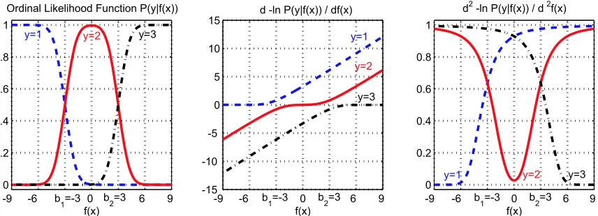
Figure 1: The graph of the likelihood function for an ordinal regression problem with r=3, along with the first and second order derivatives of the loss function (negative logarithm of the likelihood function), where the noise varianceσ2=1, and the two thresholds are b1=−3

and b2= +3.

where zi₁= byi−f(xi) σ , zi2=

b_yi−1−f(xi)

σ , andΦ(z) =R−z∞

N

(ς; 0,1)dς. Note that binary classification

is a special case of ordinal regression when r=2, and in this case the likelihood function (5) be-comes the probit function. The quantity−ln

P

(yi|f(xi))is usually referred to as the loss function

`(yi,f(xi)). The derivatives of the loss function with respect to f(xi) are needed in some

approx-imate Bayesian inference methods. The first order derivative of the loss function can be written as

∂`(yi,f(xi)) ∂f(xi)

= 1 σ

N

(zi₁; 0,1)₋

N

(zi₂; 0,1)

Φ(zi₁)₋Φ(zi₂) (6)

and the second order derivative can be given as

∂2_`(y i,f(xi)) ∂2_f(x

i)

= _σ1₂

_N

(zi₁; 0,1)₋

N

(zi₂; 0,1) Φ(zi

1)−Φ(zi2)

2

+_σ1₂z i

1

N

(zi1; 0,1)−zi2

N

(zi2; 0,1) Φ(zi

1)−Φ(zi2)

. (7)

We present graphs of the ordinal likelihood function (5) and the derivatives of the loss function in Figure 1 as an illustration. Note that the first order derivative (6) is a monotonically increasing function of f(xi), and the second order derivative (7) is always a positive value between 0 and _σ12.

Given the facts that

P

ideal(yi|f(xi) +δi) is log-concave in (f(xi),δi) and

N

(δi; 0,σ2) is also

log-concave, as pointed out by Pratt (1981), the convexity of the loss function follows, because the integral of a log-concave function with respect to some of its arguments is a log-concave function of its remaining arguments (Brascamp and Lieb, 1976, Cor. 3.5).

2.3 Posterior Probability

Based on Bayes’ theorem, the posterior probability can then be written as

P

(f_|

D

) = 1

P

(

D

) n

∏

i=1

P

(y_i|f(xi))

P

(f) (8)

where the prior probability

P

(f)is defined as in (2), the likelihood function

P

(yi|f(xi))is defined

as in (5), and

P

(

D

) =R

The Bayesian framework we described above is conditional on the model parameters including the kernel parametersκin the covariance function (1) that control the kernel shape, the threshold parameters_{b1,∆2, . . . ,∆r−1}and the noise levelσin the likelihood function (5). All these

param-eters can be collected intoθ, which is the hyperparameter vector. The normalization factor

P

(

D

)

in (8), more exactly

P

(

D

_|θ), is known as the evidence forθ, a yardstick for model selection. In the next section, we discuss techniques for hyperparameter learning.

3. Model Adaptation

In a full Bayesian treatment, the hyperparameters θmust be integrated over the θ-space. Monte Carlo methods (Neal, 1997) can be adopted here to approximate the integral effectively. However these might be prohibitively expensive to use in practice. Alternatively, we consider model se-lection by determining an optimal setting for θ. The optimal values of hyperparametersθcan be simply inferred by maximizing the posterior probability

P

(θ_|

D

), where

P

(θ_|

D

)∝

P

(

D

_|θ)

P

(θ). The prior distribution on the hyperparameters

P

(θ)can be specified by domain knowledge, or al-ternatively some vague uninformative distribution. The evidence is given by a high dimensional integral,

P

(

D

_|θ) =R

P

(

D

_|f)

P

(f)d f . A popular idea for computing the evidence is to approxi-mate the posterior distribution

P

(f_|

D

)as a Gaussian, and then the evidence can be calculated by an explicit formula (MacKay, 1992; Csat´o et al., 2000; Minka, 2001). In this section, we describe two Bayesian techniques for model adaptation by using the Laplace approximation and the expectation propagation respectively.

3.1 MAP Approach with Laplace Approximation

The evidence can be calculated analytically after applying the Laplace approximation at the max-imum a posteriori (MAP) estimate, and gradient-based optimization methods can then be used to infer the optimal hyperparameters by maximizing the evidence. The MAP estimate on the latent functions is referred to f_MAP=arg maxf

P

(f|

D

), which is equivalent to the minimizer of negative

logarithm of

P

(f_|

D

), i.e.

S

(f) = n

∑

i=1

`(yi,f(xi)) +

1 2 f

T_Σ−1_{f (9)}

where`(yi,f(xi)) =−lnP(yi|f(xi))is known as the loss function. Note that ∂ 2_S(f)

∂f∂fT =Σ−1+Λis a positive definite matrix, whereΛis a diagonal matrix whose ii-th entry is ∂2`(yi,f(xi))

∂2_f(x

i) given as in (7). Thus, this is a convex programming problem with a unique solution.3 The Laplace approximation of

S

(f) refers to carrying out the Taylor expansion at the MAP point and retaining the terms up to the second order (MacKay, 1992). Since the first order derivative with respect to f vanishes at

f_MAP,

S

(f)can also be written as

S

(f)_≈

S

(f_MAP) +1

2(f−fMAP)

T _Σ−1_+ΛMAP

(f₋f_MAP) (10) whereΛMAPdenotes the matrixΛat the MAP estimate. This is equivalent to approximating the pos-terior distribution

P

(f_|

D

)as a Gaussian distribution centered on f_MAPwith the covariance matrix

(Σ−1₊ΛMAP₎−1_{, i.e.}

_P

_(f|

_D

_)≈

_N

_{(f ; f}

MAP,(Σ−1+ΛMAP)−1). Using the Laplace approximation

(10) and

Z

f defined as in (2), the evidence can be computed analytically as follows

P

(

D

_|θ) = 1

Z

f

Z

exp(₋

S

(f))d f _≈exp(₋

S

(f_MAP))_|I+ΣΛMAP_|−12 ₍₁₁₎

where I is an n_×n identity matrix. The gradients of the logarithm of the evidence (11) with respect to the hyperparametersθcan be derived analytically. Then gradient-based optimization methods can be employed to search for the maximizer of the evidence. Refer to Appendix A for the detailed gradient formulae and the outline of our algorithm for model adaptation.

3.2 Expectation Propagation with Variational Methods

The expectation propagation algorithm (EP) is an approximate Bayesian inference method (Minka, 2001), which can be regarded as an extension of assumed-density-filter (ADF). The EP algorithm has been applied in Gaussian process classification along with variational methods for model selec-tion (Seeger, 2002; Kim and Ghahramani, 2003). In the setting of Gaussian processes, EP attempts to approximate

P

(f_|

D

)as a product distribution in the form of Q(f) =∏n_i=1˜ti(f(xi))

P

(f)where

˜ti(f(xi)) =siexp(−1₂pi(f(xi)−mi)2). The parameters{si,mi,pi}in{˜ti}are successively optimized

by minimizing the following Kullback-Leibler divergence,

˜tnew

i =arg min ˜ti

KL

Q(f)

˜told i

P

(y_i|f(xi))

Q(f)

˜told i

˜ti

. (12)

Since Q(f)is in the exponential family, this minimization can be simply solved by moment match-ing up to the second order. A detailed updatmatch-ing scheme can be found in Appendix B. At the equilibrium of Q(f), we obtain an approximate posterior distribution as

P

(f_|

D

)_≈

N

(f ;(Σ−1₊ Π)−1Π_m,(Σ−1₊Π₎−1_)whereΠ_{is a diagonal matrix whose ii-th entry is p}

iand m= [m1,m2, . . . ,mn]T.

Variational methods can be used to optimize the hyperparameters θby maximizing the lower bound on the logarithm of the evidence. By applying Jensen’s inequality, we have

log

P

(

D

_|θ) =logR P(D|f)P(f)

Q(f) Q(f)d f ≥

R

Q(f)logP(D_Q|₍f_f)P₎(f)d f

=R

Q(f)log

P

(

D

_|f)d f+R

Q(f)log

P

(f)d f−R

Q(f)log Q(f)d f =

F

(θ). (13) The lower bound

F

(θ)can be written as an explicit expression at the equilibrium of Q(f), and then the gradients with respect toθcan be derived by neglecting the possible dependency of Q(f)onθ. The detailed formulation can be found in Appendix C.

4. Prediction

We have described two techniques, the MAP approach and the EP approach, to infer the optimal model. At the optimal hyperparameters we inferred, denoted as θ∗, let us take a test case x for which the target yxis unknown. The latent variable f(x)and the column vector f containing the n

zero-mean random variables_{f(xi)}n_i=1have the prior joint multivariate Gaussian distribution, i.e.

f f(x)

∼

N

0 0

,

Σ

k

kT

K

(x,x)

where k= [

K

(x,x1),

K

(x,x2), . . . ,

K

(x,xn)]T. The conditional distribution of f(x) given f is a

Gaussian too, denoted as

P

(f(x)_|f,θ∗)with mean fTΣ−1k and variance

K

(x,x)₋kTΣ−1k. The predictive distribution of

P

(f(x)_|

D

,θ∗)can be computed as an integral over f -space, which can be written as

P

(f(x)_|

D

,θ∗) =

Z

P

(f(x)_|f,θ∗)

P

(f_|

D

,θ∗)d f. (14) The posterior distribution

P

(f_|

D

,θ∗)can be approximated as a Gaussian by the MAP approach or the EP approach (refer to Section 3). The predictive distribution (14) can then be simplified as a Gaussian

N

(f(x); µx,σ2x)with mean µxand varianceσ2x. In the MAP approach, we reach

µx=kTΣ−1fMAP and σ2x=

K

(x,x)−kT(Σ+ΛMAP−1 )−1k. (15)

While in the EP approach, we get

µx=kT(Σ+Π−1)−1m and σ2x=

K

(x,x)−kT(Σ+Π−1)−1k. (16)

The predictive distribution over ordinal targets yx is

P

(yx|x,

D

,θ∗) =R

P

(yx|f(x),θ∗)

P

(f(x)_|

D

,θ∗)d f(x) =Φ

byx−µx

√

σ2_+σ2

x

−Φ

byx−1−µx

√

σ2_+σ2

x

.

The predictive ordinal scale can be decided as arg max

i

P

(yx=i|x,

D

,θ ∗_).

5. Discussion

In the MAP approach, the mean of the predictive distribution depends on the MAP estimate f_MAP, which is unique and can be found by solving a convex programming problem. Evidence maximiza-tion is useful if the Laplace approximamaximiza-tion around the mode point f_MAPgives a good summary of the posterior distribution

P

(f_|

D

). While in the approach of expectation propagation, the mean of the predictive distribution depends on the approximate mean of the posterior distribution. When the true shape of

P

(f|

D

)is far from a Gaussian centered on the mode, the EP approach can have a great advantage over the Laplace approximation. However the EP algorithm cannot guarantee convergence, though it usually works well in practice.

The gradient-based optimization method usually requests evidence evaluation at tens of different settings ofθbefore the minimum is found. For eachθ, the inversion of the matrixΣis required that costs time at

O

(n3), where n is the number of training samples. Recently, Csat´o and Opper (2002) proposed a fast training algorithm for Gaussian processes in which the set of basis vectors are determined on-line for sparse representation. Lawrence et al. (2003) proposed a greedy selection with criteria based on information-theoretic principles for sparse Gaussian processes (Seeger, 2003). Tresp (2000) proposed the Bayesian committee machines to divide and conquer large data sets, while using infinite mixtures of Gaussian Processes (Rasmussen and Ghahramani, 2002) is another promising technique. These algorithms can be applied directly in the settings of ordinal regression for speedup.

into the covariance function (1) as follows:

Cov[f(xi),f(xj)] =

K

(xi,xj) =exp −

1 2

d

∑

ς=1

κς(xς_i−xς_j)2

!

(17)

whereκς>0 is the ARD parameter.4 The gradients with respect to the variables_{lnκς}can also be derived analytically for model adaptation. The optimal value of the ARD parameterκ_ςindicates the relevance of the ς-th input feature to the target. The form of feature selection we use here results in a type of feature weighting. Furthermore, the linear combination of heterogeneous kernels with positive coefficients is still a valid covariance function. Lanckriet et al. (2004) suggest to learn the kernel matrix with semidefinite programming. In the Bayesian framework, these positive coefficients for kernels could be treated as hyperparameters, and optimized using the evidence as a criterion for optimization.

Note that binary classification is a special case of ordinal regression with r=2, and the like-lihood function (5) becomes the probit function when r=2. Both of the probit function and the logistic function can be used as the likelihood function in binary classification, while they have different origins. Due to the dichotomous nature in the classes of multi-classification, discriminant functions are constructed for each class and then compete again others via the softmax function to determine the likelihood. The logistic function, as a special case of the softmax function, comes from general classification problems.

In metric regression, warped Gaussian processes (Snelson et al., 2004) assume that there is a nonlinear, monotonic, and continuous warping function relating the observed targets and some latent variables in a Gaussian process. The warping function, which is learned from the data, can be thought of as a pre-processing transformation applied before modelling with a Gaussian process. A different (and very common) approach to dealing with this preprocessing is to discretize the target values into r different bins. These discrete values are clearly ordinal, and applying ordinal regression to these discrete values seems the natural choice. Interestingly, as the number of discretization bins r is increased, the ordinal regression model becomes very similar to the warped Gaussian processes model. In particular, by varying the thresholds in our ordinal regression model, it can approximate any continuous warping function.

6. Numerical Experiments

We start this section with a simple synthetic data set to visualize the behavior of these algorithms, and report the experimental results on sixteen benchmark data sets.5 Then we perform experiments on a collaborative filtering problem using the “EachMovie” data, and on Gleason score prediction from gene microarray data related to prostate cancer. Shashua and Levin (2003) generalized the sup-port vector formulation by finding multiple thresholds to define parallel discriminant hyperplanes for ordinal scales, and reported that the performance of the support vector approach is better than that of the on-line algorithm (Crammer and Singer, 2002). The problem size in the large-margin ranking algorithm of Herbrich et al. (2000) is a quadratic function of the training data size making the algorithmic complexity

O

(n4)–O(n6). This makes the experiments on large data sets computa-tionally difficult. Thus, we decide to limit our comparisons to the support vector approach (SVM)

of Shashua and Levin (2003) and the two versions of our approach, the MAP approach with Laplace approximation (MAP) and the EP algorithm with variational methods (EP). In our implementation,6 we used the routine L-BFGS-B (Byrd et al., 1995) as the gradient-based optimization package, and started from the initial values of hyperparameters to infer the optimal values in the criterion of the approximate evidence (11) for MAP or the variational lower bound (13) for EP respectively.7 The improved SMO algorithm (Keerthi et al., 2001) was adapted to implement the SVM approach (refer to Chu and Keerthi (2005) for detailed description and extensive discussion),8_{and 5-fold cross}

vali-dation was used to determine the optimal values of model parameters (the kernel parameterκand the regularization factor C) involved in the problem formulations. The initial search was done on a 7_×7 coarse grid linearly spaced in the region_{(log₁₀C,log₁₀κ)_{| −}3_≤log₁₀C_≤3,₋3_≤log₁₀κ_≤3_}, followed by a fine search on a 9_×9 uniform grid linearly spaced by 0.2 in the (log₁₀C,log₁₀κ)

space. We have utilized two evaluation metrics which quantify the accuracy of predictive ordinal scales_{yˆ1, . . . ,yˆt}with respect to true targets{y1, . . . ,yt}:

• Mean absolute error is the average deviation of the prediction from the true target, i.e.

1 t ∑

t

i=1|yˆi−yi|, in which we treat the ordinal scales as consecutive integers;

• Mean zero-one error gives an error of 1 to every incorrect prediction that is the fraction of incorrect predictions.

6.1 Artificial Data

Figure 2 presents the behavior of the three algorithms using the Gaussian kernel (1) on a synthetic 2D data with three ordinal scales. In the support vector approach, the optimal thresholds were determined by the SMO algorithm and 5-fold cross validation was used to decide the optimal values of the kernel parameter and the regularization factor. As for the Gaussian process algorithms, model adaptation (see Section 3) was used to determine the optimal values of the kernel parameter, the noise level and the thresholds automatically. The figure shows that all the algorithms are working reasonably well on this task.

6.2 Benchmark Data

We collected nine benchmark data sets (Set I in Table 1) that were used for metric regression prob-lems. The target values were discretized into ordinal quantities using equal-length binning. These bins divide the range of target values into a given number of intervals that are of same length. The resulting rank values are ordered, representing these intervals of the original metric quantities. For each data set, we generated two versions by discretizing the target values into five and ten intervals respectively. We randomly partitioned each data set into training/test splits as specified in Table 1. The partition was repeated 20 times independently. The Gaussian kernel (1) was used in these three algorithms. The test results are recorded in Tables 2 and 3. The performance of the MAP and EP approaches are closely matching. Our Gaussian process algorithms often yield better results than

6. The two versions of our proposed approach were implemented in ANSI C, and the source code is accessible at http://www.gatsby.ucl.ac.uk/∼chuwei/code/gpor.tar.

7. In numerical experiments, the initial values of the hyperparameters were usually chosen asσ2=1,κ=1/d for

Gaussian kernel, the threshold b1=−1 and∆ι=2/r. We suggest to try several starting points in practice, and then

choose the best model by the objective functional.

0 1 2 3 4 −3

−2 −1 0 1 2 3

Lower Noise

The SVM Approach

−40.37

−26.79

0 1 2 3 4 −3

−2 −1 0 1 2 3

The MAP Approach

−1.01 0.46

0 1 2 3 4 −3

−2 −1 0 1 2 3

The EP Approach

−2.33 −0.96

0 1 2 3 4 −3

−2 −1 0 1 2 3

Higher Noise

The SVM Approach

−27.83

−22.96

0 1 2 3 4 −3

−2 −1 0 1 2 3

The MAP Approach

−1.56 −0.44

0 1 2 3 4 −3

−2 −1 0 1 2 3

The EP Approach

−3.22 −1.26

Figure 2: The performance of the three algorithms on a synthetic three-rank ordinal regression problem. The discriminant function values of the SVM approach, and the predictive mean values of the two Gaussian process approaches are presented as contour graphs in-dexed by the two thresholds. The upper graphs are for the case of lower noise level, while the lower graphs are for the case of higher noise level. The training samples we used are presented in these graphs. The dots denote the training samples of rank 1, the crosses denote the training samples of rank 2 and the circles denote the training samples of rank 3.

the support vector approach on the average value, especially when the number of training samples is small.

In the next experiment, we selected seven very large metric regression data sets (Set II in Table 1). The input vectors were normalized to zero mean and unit variance coordinate-wise. The target values of these data sets were discretized into 10 ordinal quantities using equal-frequency binning. For each data set, a small subset was randomly selected for training and then tested on the remaining samples, as specified in Table 1. The partition was repeated 100 times independently. To show the advantage of explicitly modelling the ordinal nature of the targets, we also employed the standard Gaussian process algorithm (Williams and Rasmussen, 1996) for metric regression (GPR)9to tackle these ordinal regression tasks, where the ordinal targets were naively treated as continuous values and the predictions for test cases were rounded to the nearest ordinal scale. The Gaussian kernel (1) was used in the four algorithms. From the test results in Table 4, the ordinal regression

Data Sets Attributes(Numeric,Nominal) Training Instances Instances for Test

Diabetes 2(2,0) 30 13

Pyrimidines 27(27,0) 50 24

Triazines 60(60,0) 100 86

Wisconsin Breast Cancer 32(32,0) 130 64

Set I Machine CPU 6(6,0) 150 59

Auto MPG 7(4,3) 200 192

Boston Housing 13(12,1) 300 206

Stocks Domain 9(9,0) 600 350

Abalone 8(7,1) 1000 3177

Bank Domains(1) 8(8,0) 50 8142

Bank Domains(2) 32(32,0) 75 8117

Computer Activity(1) 12(12,0) 100 8092

Set II Computer Activity(2) 21(21,0) 125 8067

California Housing 8(8,0) 150 15490

Census Domains(1) 8(8,0) 175 16609

Census Domains(2) 16(16,0) 200 16584

Table 1: Data sets and their characteristics. “Attributes” state the number of numerical and nominal attributes. “Training Instances” and “Instances for Test” specify the size of training/test partition. The partitions we generated and the test results on individual partitions can be accessed at http://www.gatsby.ucl.ac.uk/_∼chuwei/ordinalregression.html.

Mean zero-one error Mean absolute error

Data SVM MAP EP SVM MAP EP

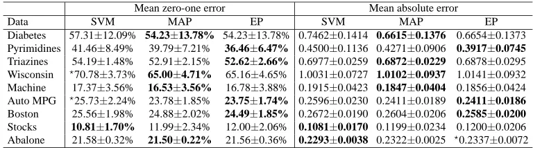
Diabetes 57.31±12.09% 54.23±13.78% 54.23±13.78% 0.7462±0.1414 0.6615±0.1376 0.6654±0.1373 Pyrimidines 41.46±8.49% 39.79±7.21% 36.46±6.47% 0.4500±0.1136 0.4271±0.0906 0.3917±0.0745

Triazines 54.19±1.48% 52.91±2.15% 52.62±2.66% 0.6977±0.0259 0.6872±0.0229 0.6878±0.0295 Wisconsin ?_{70.78±3.73% 65.00±4.71% 65.16±4.65% 1.0031±0.0727 1.0102±0.0937 1.0141±0.0932}

Machine 17.37±3.56% 16.53±3.56% 16.78±3.88% 0.1915±0.0423 0.1847±0.0404 0.1856±0.0424 Auto MPG ?25.73±2.24% 23.78±1.85% 23.75±1.74% 0.2596±0.0230 0.2411±0.0189 0.2411±0.0186

Boston 25.56±1.98% 24.88±2.02% 24.49±1.85% 0.2672±0.0190 0.2604±0.0206 0.2585±0.0200

Stocks 10.81±1.70% 11.99±2.34% 12.00±2.06% 0.1081±0.0170 0.1199±0.0234 0.1200±0.0206 Abalone 21.58_±0.32% 21.50_±0.22% 21.56_±0.36% 0.2293_±0.0038 0.2322_±0.0025 ?_{0.2337±0.0072} Table 2: Test results of the three algorithms using a Gaussian kernel. The targets of these

bench-mark data sets were discretized by 5 equal-length bins. The results are the averages over 20 trials, along with the standard deviation. We use the bold face to indicate the cases in which the average value is the lowest in the results of the three algorithms. The symbols ?are used to indicate the cases in which the indicated entry is significantly worse than the winning entry; A p-value threshold of 0.01 in Wilcoxon rank sum test was used to decide statistical significance.

Mean zero-one error Mean absolute error

Data SVM MAP EP SVM MAP EP

Diabetes ?90.38±7.00% 83.46±5.73% 83.08±5.91% 2.4577±0.4369 2.1385±0.3317 2.1423±0.3314 Pyrimidines 59.37_±7.63% 55.42_±8.01% 54.38_±7.70% 0.9187_±0.1895 0.8771_±0.1749 0.8292_±0.1338

Triazines ?67.91±3.63% 63.72±4.34% 64.01±3.78% 1.2308±0.0874 1.1994±0.0671 1.2012±0.0680 Wisconsin ?85.86±3.78% 78.52±3.58% 78.52±3.51% 2.1250±0.1500 2.1391±0.1797 2.1437±0.1790 Machine 32.63±3.84% 33.81±3.91% 33.73±3.64% 0.4398±0.0688 0.4746±0.0727 0.4686±0.0763 Auto MPG 44.01±2.30% 43.96±2.81% 43.88±2.60% 0.5081±0.0263 0.4990±0.0352 0.4979±0.0340

Boston 42.06_±2.49% 41.53_±2.77% 41.26_±2.86% 0.4971_±0.0305 0.4920_±0.0330 0.4896_±0.0346

Stocks 17.74±2.15% ?19.90±1.72% ?19.44±1.91% 0.1804±0.0213 ?0.2006±0.0166 ?0.1960±0.0184 Abalone 42.84±0.86% 42.60±0.91% 42.27±0.46% 0.5160±0.0087 0.5140±0.0075 0.5113±0.0053 Table 3: Test results of the three algorithms using a Gaussian kernel. The targets of these

bench-mark data sets were discretized by 10 equal-length bins. The results are the averages over 20 trials, along with the standard deviation. We use the bold face to indicate the cases in which the average value is the lowest in the results of the three algorithms. The symbols ?are used to indicate the cases in which the indicated entry is significantly worse than the winning entry; A p-value threshold of 0.01 in Wilcoxon rank sum test was used to decide statistical significance.

Mean zero-one error NLL

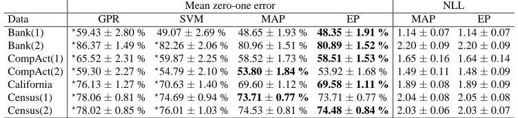
Data GPR SVM MAP EP MAP EP

Bank(1) ?59.43±2.80 % 49.07±2.69 % 48.65±1.93 % 48.35±1.91 % 1.14±0.07 1.14±0.07 Bank(2) ?86.37_±1.49 % ?82.26_±2.06 % 80.96_±1.51 % 80.89_±1.52 % 2.20_±0.09 2.20_±0.09 CompAct(1) ?65.52±2.31 % ?59.87±2.25 % 58.52±1.73 % 58.51±1.53 % 1.65±0.16 1.64±0.14 CompAct(2) ?59.30±2.27 % ?54.79±2.10 % 53.80±1.84 % 53.92±1.68 % 1.49±0.11 1.48±0.09 California ?76.13±1.27 % ?70.63±1.40 % 69.60±1.12 % 69.58±1.11 % 1.89±0.08 1.89±0.09 Census(1) ?78.06±0.81 % ?74.69±0.94 % 73.71±0.77 % 73.71±0.77 % 2.04±0.08 2.05±0.08 Census(2) ?78.02±0.85 % ?76.01±1.03 % 74.53±0.81 % 74.48±0.84 % 2.03±0.06 2.03±0.07

Table 4: Test results of the four algorithms using a Gaussian kernel. The targets of these bench-mark data sets were discretized by 10 equal-frequency bins. The results are the average over 100 trials, along with the standard deviation. “GPR” denotes the standard algorithm of Gaussian process metric regression that treats the ordinal scales as continuous values. “NLL” denotes the negative logarithm of the likelihood in prediction. We use the bold face to indicate the cases in which the average value is the lowest mean zero-one error of the four algorithms. The symbols?are used to indicate the cases in which the indicated entry is significantly worse than the winning entry; A p-value threshold of 0.01 in Wilcoxon rank sum test was used to decide statistical significance.

6.3 Collaborative Filtering

Collaborative filtering exploits correlations between ratings across a population of users. The goal is to predict a person’s rating on new items given the person’s past ratings on similar items and the ratings of other people on all the items (including the new item). The ratings are ordered, making collaborative filtering an ordinal regression problem. We carried out ordinal regression on a subset of the EachMovie data (Compaq, 2001).10 The rates given by the user with ID number “52647” on 449 movies were used as the targets, in which the numbers of zero-to-five star are 40, 20, 57, 113, 145 and 74 respectively. We selected 1500 users who contributed the most ratings on these 449 movies as the input features. The ratings given by the 1500 users on each movie were used as the input vector accordingly. In the 449_×1500 input matrix, about 40% elements were observed. We randomly selected a subset with size _{50,100, . . . ,300_} of the 449 movies for training, and then tested on the remaining movies. At each size, the random selection was carried out 20 times independently.

Pearson correlation coefficient is the most popular correlation measure (Basilico and Hofmann, 2004), which corresponds to a dot product between normalized rating vectors. For instance, if applied to the movies, we can define the so-called z-scores as

z(v,u) =r(v,u)−µ(v) σ(v)

where u indexes users, v indexes movies, and r(v,u)is the rating on the movie v given by the user u. µ(v)andσ(v)are the movie-specific mean and standard deviation respectively. This correlation coefficient, defined as

K

(v,v0) =

∑

u

z(v,u)z(v0,u)

where∑u denotes summing over all the users, was used as the covariance/kernel function in our experiments for the three algorithms. As not all ratings are observed in the input vectors, we con-sider two ad hoc strategies to deal with missing values: mean imputation and weighted low-rank approximation. In the first case, unobserved values are identified with the mean value, that means their corresponding z-score is zero. In the second case, we applied the EM procedure described by Srebro and Jaakkola (2003) to fill in the missing data with the estimate. In the input matrix, observed elements were weighted by one and missing data were given weight zero. The low rank was fixed at 2. In Figure 3, we present the test results of the two cases at different training data size. Using mean imputation, SVM produced a bit more accurate results than Gaussian processes on mean absolute error. In the cases with low rank approximation as preprocessing, the performance of the three algorithms are highly competitive, and more interestingly, we observed about 0.08 im-provement on mean absolute error for all the three algorithms. A serious treatment on the missing data could be an interesting research topic for future work.

6.4 Gene Expression Analysis

Singh et al. (2002) carried out microarray expression analysis on 12600 genes to identify genes that might anticipate the clinical behavior of prostate cancer. Fifty-two samples of prostate tumor were investigated. For each sample, the Gleason score ranging from 6 to 10, was given by the

50 100 150 200 250 300 0.6

0.65 0.7 0.75 0.8 0.85 0.9 0.95 1

Mean absolute error

Training data size with Mean Imputation

50 100 150 200 250 300

0.6 0.65 0.7 0.75 0.8 0.85 0.9 0.95 1

Training data size

with Weighted Low−rank Approximation

50 100 150 200 250 300 0.5

0.55 0.6 0.65 0.7

Mean zero−one error

Training data size 50 100 150 200 250 300 0.5

0.55 0.6 0.65 0.7

Training data size

1 3 5 10 40 200 1000 12600 0

0.1 0.2 0.3 0.4 0.5 0.6

The SVM Approach

Number of selected genes

Mean zero−one error

1 3 5 10 40 200 1000 12600 0

0.1 0.2 0.3 0.4 0.5 0.6

The MAP Approach

Number of selected genes

1 3 5 10 40 200 1000 12600 0

0.1 0.2 0.3 0.4 0.5 0.6

The EP Approach

Number of selected genes

1 3 5 10 40 200 1000 12600 0

0.1 0.2 0.3 0.4 0.5 0.6

The SVM Approach

Number of selected genes

Mean absolute error

1 3 5 10 40 200 1000 12600 0

0.1 0.2 0.3 0.4 0.5 0.6

The MAP Approach

Number of selected genes

1 3 5 10 40 200 1000 12600 0

0.1 0.2 0.3 0.4 0.5 0.6

The EP Approach

Number of selected genes

pathologist reflecting the level of differentiation of the glands in the prostate tumor. Predicting the Gleason score from the gene expression data is thus a typical ordinal regression problem. Since only 6 samples had a score greater than 7, we merged them as the top level, leading to three levels

{=6,=7,_≥8} with 26, 20 and 6 samples respectively. We randomly partitioned the data into 2 folds for training and test and repeated this partitioning 20 times independently. An ARD linear kernel

K

(xi,xj) =∑d_ς=1κςxςix

ς

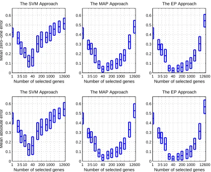
j was used to evaluate feature relevance. These ARD parameters {κς} were optimized by evidence maximization. According to the optimal values of these ARD parameters, the genes were ranked from irrelevant to relevant. We then removed the irrelevant genes gradually based on the rank list. The gene number was reduced from 12600 to 1. At each number of selected genes, a linear kernel

K

(xi,xj) =∑d_ς=1x

ς

ix

ς

j was used in the three algorithms for

a fair comparison. Figure 4 presents the test results of the three algorithms for different numbers of selected genes. We observed great and steady improvement using the subset of genes selected by the ARD technique. The best validation output is achieved around 40 top-ranked features. In this case, with only 26 training samples, the Bayesian approaches perform much better than the SVM, and the EP approach is generally better than the MAP approach but the difference is not statistically significant.

7. Conclusion

Ordinal regression is an important supervised learning problem with properties of both metric re-gression and classification. In this paper, we proposed a simple yet novel nonparametric Bayesian approach to ordinal regression based on a generalization of the probit likelihood function for Gaus-sian processes. Two approximate inference procedures were derived in detail for evidence evalua-tion and model adaptaevalua-tion. The approach intrinsically incorporates ARD feature selecevalua-tion and pro-vides probabilistic prediction. The existent fast algorithms for Gaussian processes can be adapted directly to tackle relatively large data sets. Experiments on benchmark and real-world data sets show that the generalization performance is competitive and often better than support vector methods.

Acknowledgments

The main part of this work was carried out at Institute for Pure and Applied Mathematics (IPAM) of UCLA. We thank David L. Wild for stimulating this work and for many discussions. We also thank David J. C. MacKay for valuable comments. Wei Chu was supported by the National Institutes of Health and its National Institute of General Medical Sciences division under Grant Number 1 P01 GM63208. Zoubin Ghahramani was partially supported from CMU by DARPA under the CALO project. The reviewers’ thoughtful comments are gratefully appreciated.

Appendix A. Gradient Formulae for Evidence Maximization

Evidence maximization is equivalent to finding the minimizer of the negative logarithm of the evi-dence which can be written in an explicit expression as follows

−lnP(

D

_|θ)_≈ n

∑

i=1

`(yi,fMAP(xi)) +

1 2 f

T

MAPΣ−1fMAP+

1

Initialization choose a favorite gradient-descent optimization package select the starting pointθfor the optimization package

Looping while the optimization package requests evidence/gradient evaluation atθ 1. find the MAP estimate by solving the convex programming problem (9) 2. evaluate the negative logarithm of the evidence (18) at the MAP 3. calculate the gradients with respect toθ(18)–(18)

4. feed the evidence and gradients to the optimization package Exit Return the optimalθfound by the optimization package

Table 5: The outline of our algorithm for model adaptation using the MAP approach with Laplace approximation.

We usually collect_{lnκ,lnσ,b1,ln∆2, . . . ,ln∆r−1}as the set of variables to tune. This definition of

tunable variables is helpful to convert the constrained optimization problem into an unconstrained optimization problem. The outline of our algorithm for model adaptation is described in Table 5.

The derivatives of₋ln

P

(

D

_|θ)with respect to these variables can be derived as follows:

∂−lnP(

D

_|θ) ∂lnκ =

κ

2trace

(Λ−1

MAP+Σ)−1 ∂Σ ∂κ −κ 2 f T MAPΣ−1

∂Σ

∂κΣ−1fMAP +κ

2trace

Λ−1 MAP(Λ−

1

MAP+Σ)−

1_Σ∂ΛMAP ∂κ

;

∂−lnP(

D

_|θ) ∂lnσ =σ

n

∑

i=1

∂`(yi,fMAP(xi))

∂σ +

σ

2trace

Λ−1

MAP(Λ−MAP1 +Σ)−1Σ ∂ΛMAP

∂σ

;

∂−ln

P

(

D

_|θ) ∂b1

= n

∑

i=1

∂`(yi,fMAP(xi)) ∂b1

+1

2trace

Λ−1

MAP(Λ−MAP1 +Σ)−1Σ ∂ΛMAP

∂b1

;

∂−lnP(

D

_|θ) ∂ln∆ι =∆ι

n

∑

i=1

∂`(yi,fMAP(xi)) ∂∆ι +

∆ι 2trace

Λ−1

MAP(Λ−MAP1 +Σ)−1Σ ∂ΛMAP

∂∆ι

.

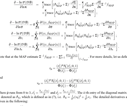
Note that at the MAP estimateΣ−1f_MAP=₋∑n i=1 ∂`

(yi,f(xi)) ∂f

f=fMAP

. For more details, let us define

s_ρ=(z i

1)ρ

N

(zi1; 0,1) Φ(zi₁)₋Φ(zi₂)

and

v_ρ=(z i

1)ρ

N

(zi1; 0,1)−(zi2)ρ

N

(zi2; 0,1) Φ(zi₁)₋Φ(zi₂)

whereρruns from 0 to 3, zi₁=byi−f(xi)

σ and zi2=

b_yi−1−f(xi)

σ . The ii-th entry of the diagonal matrixΛ is denoted asΛii, which is defined as in (7), i.e. Λii=_σ12(v0)2+

1

σ2v1. The detailed derivatives are

given in the following:

• ∂Λii_∂κ =∂Λii_∂fT ∂f

∂κ.

• _∂∂Λiif(xi)=

1

• ∂_∂κf =Λ−1₍Λ−1₊Σ₎−1∂Σ

∂κΣ−1f .

• ∂`(yi,f(xi)) ∂σ =vσ1.

• ∂Λii_∂σ =₋2

σΛii+σ13(2v0v2+2(v0)2v1−v1+ (v1)2+v3) +∂Λii_∂fT∂

f

∂σ.

• ∂_∂σf =Λ−1₍Λ−1₊Σ₎−1Σψ

σ, whereψσis a column vector whose i-th element is σ12(v0−v0v1−

v2). • ∂Λii_∂b1 =−

∂Λii ∂f(xi)+

∂Λii ∂fT ∂

f

∂b1.

• _∂∂bf1 =Λ

−1₍Λ−1₊Σ₎−1Σψ

b, whereψbis a column vector whose i-th element isΛii.

• ∂`(yi,f(xi))

∂∆ι =







−v0

σ if yi>ι; −s0

σ if yi=ι;

0 otherwise.

• ∂Λii_∂∆ι =



  

  

−_∂∂Λiif(xi)+ ∂Λii ∂fT

∂f

∂∆ι if yi>ι;

ϕi+∂Λii_∂f ∂_∂∆fT

ι if yi=ι; ∂Λii

∂f

∂fT

∂∆ι otherwise.

• ϕi= ∂Λii_∂∆

ι =

1

σ3(s0−2v0s1−2(v0)2s0−s2−v1s0). • _∂∆∂f_ι =Λ−1_(Λ−1_+Σ)−1_Σψ

∆, whereψ∆ is a column vector whose i-th element is defined as

ψi

∆=







Λiii.e. _σ12((v0)2+v1) if yi>ι; 1

σ2(v0s0+s1) if yi=ι;

0 otherwise.

Appendix B. Approximate Posterior Distribution by EP

The expectation propagation algorithm attempts to approximate

P

(f|

D

) in form of a product of Gaussian distributions Q(f) =∏n_i=1˜t(f(xi))

P

(f)where ˜t(f(xi)) =siexp(−1₂pi(f(xi)−mi)2). The

updating scheme is given as follows.

The initial states:

• individual mean mi=0∀i ;

• individual inverse variance pi=0∀i ;

• individual amplitude si=1∀i ;

• posterior covariance

A

= (Σ−1₊Π₎−1_{, where}Π_=diag(p

1,p2, . . . ,pn) ; • posterior mean h=

A

Πm, where m= [m1,m2, . . . ,mn]T .

Looping i from 1 to n until there is no significant change in{mi,pi,si}ni=1:

– variance of f(xi):λ\ii=

Aii

1₋Aiipi ;

– mean of f(xi): h\ i

i =hi+λ\ i

i pi(hi−mi) ; – others with j₆=i:λ\_ji=

A

_{j j}and h\_ji=hj .

• ˜t(f(xi))in Q(f)is updated by incorporating the message

P

(yi|f(xi))into Q\i(f):

–

Z

_i=R

P

(y_i|f(xi))

N

(f(xi); h\ii,λ\ i

i )d f(xi) =Φ(˜z1)−Φ(˜z2)

where ˜z1= b_yi−h\_ii

q λ\i

i +σ2

and ˜z2=

b_yi−1−h\ii q

λ\i i +σ2

.

– βi=∂log_∂λ\Zii i

=₋ 1 2(λ\_ii+σ2₎

_˜z

1N(˜z1;0,1)−˜z2N(˜z2;0,1)

Φ(˜z1)−Φ(˜z2)

.

γi=∂logZi ∂h\_ii =−

1

q λ\i

i +σ2

_N(˜z

1;0,1)−N(˜z2;0,1)

Φ(˜z1)−Φ(˜z2)

. ₍₁₈₎

– υi=γ2 i −2βi. – hnew_i =h\_ii+λ\_iiγi .

– pnew_i = υi 1−λ\iiυi

.

– mnew_i =h\_ii+_υiγi .

– snew_i =

Z

_i

q

λ\i

i pnewi +1 exp

_γ2

i

2υi

.

• Note that pnew_i >0 all the time, because 0<υi< 1 λ\i

i+σ2

and thenλ\_iiυi<1.

• if pnew_{i ≈}pi, skip this sample and this updating; otherwise update{pi,mi,si}, the posterior

mean h and covariance

A

as follows:

–

A

new₌

_A

_−ρa

iaTi whereρ= pnew

i −pi

1+(pnew

i −pi)Aii and aiis the i-th column of

A.

– hnew=h+ηai whereη=γi+₁p₋i(Ahiii−pimi)andγiis defined as in (18).

As a byproduct, we can get the approximate evidence

P

(

D

_|θ) at the EP solution, which can be written as

n

∏

i=1

si

det12(Π−1)

det12(Σ+Π−1)

exp

B 2

where B=∑i j

A

_{i j}(mipi)(mjpj)−∑ipim2i.

Appendix C. Gradient Formulae for Variational Bound

At the equilibrium of Q(f), the variational bound

F

(θ)can be analytically calculated as follows:

F

(θ) = n

∑

i=1

Z

N

(f(xi); hi,

A

ii)ln(

P

(yi|f(xi)))d f(xi)−

1

2ln|I+ΣΠ|

−1₂trace((I+ΣΠ)−1)₋1

2m

T_(Σ+Π−1₎₋1_Σ(Σ+Π−1₎₋1_m+n

Note that(Σ+Π−1₎−1_{m can be directly obtained by{}γi}_{defined as in (18). The gradient of}

_F

₍θ₎

with respect to the variables_{lnκ,lnσ,b1,ln∆2, . . . ,ln∆r₋1}can be given in the following:

∂F(θ)

∂lnκ =κ

Z

Q(f)∂log

P

(f) ∂κ d f =₋κ

2trace

Σ−1∂Σ ∂κ

+κ

2h

T_Σ−1∂Σ

∂κΣ−1h+ κ

2trace

Σ−1∂Σ ∂κΣ−1

A

=₋κ

2trace

(Π−1+Σ)−1∂Σ ∂κ

+κ

2m

T_(Π−1_+Σ)−1∂Σ

∂κ(Π−1+Σ)−1m,

∂F(θ)

∂lnσ =σ∑ n i=1

R

N

(f(xi); hi,

A

ii)∂ln

P(yi|f(xi)) ∂σ d f(xi)

=−∑_{1≤yi<r}R

N

f(xi);

hiσ2+Aiib_yi σ2_+A

ii , σ2_A

ii σ2_+A

ii

byi−f(_xi)

√ 2π(σ2_+A

ii)

exp

−(₂hi_(σ−2_+Abyi)2

ii)

P(yi|f(xi)) d f(xi)

+∑_{1<yi≤r}R

N

f(xi);

hiσ2+Aiib_yi−1

σ2_+A

ii , σ2_A

ii σ2_+A

ii

by_i−1−f(xi) √

2π(σ2_+A

ii)

exp

−(hi−byi−1)

2

2(σ2_+A

ii)

P(yi|f(xi)) d f(xi), ∂F(θ)

∂b1 =∑ n i=1

R

N

(f(xi); hi,

A

ii)∂ln

P(yi|f(xi)) ∂b1 d f(xi)

=∑_{1_≤yi<r_}

R

N

(f(xi); hiσ2_+A

iib_yi σ2_+A

ii , σ2_A

ii σ2_+A

ii)

1 √

2π(σ2₊A_ii)

exp

−₂(hi_(σ−2_+Abyi)2

ii)

P(yi|f(xi) d f(xi)

−∑_{1<yi≤r}

R

N

(f(xi); hiσ2_+A

iib_yi−1

σ2_+A

ii , σ2_A

ii σ2_+A

ii)

1 √

2π(σ2_+A

ii)

exp

−(hi−byi−1)

2

2(σ2_+A

ii)

P(yi|f(xi)) d f(xi), ∂F(θ)

∂ln∆ι =∆ι∑

n i=1

R

N

(f(xi); hi,

A

ii)∂ln

P(yi|f(xi)) ∂∆ι d f(xi)

=∆ι∑_{ι≤yi<r}

R

N

(f(xi); hiσ2_+A

iib_yi σ2_+A

ii , σ2_A

ii σ2_+A

ii)

1 √

2π(σ2₊A_ii)

exp

−₂(hi_(σ−2byi_+A)2

ii)

P(yi|f(xi) d f(xi)

−∆ι∑{ι<yi≤r}

R

N

(f(xi);

hiσ2+Aiib_yi−1

σ2_+A

ii , σ2_A

ii σ2_+A

ii)

1 √

2π(σ2_+A

ii)

exp

−(hi−byi−1)

2

2(σ2_+A

ii)

P(yi|f(xi)) d f(xi), where∑_{ι<yi≤r}means summing over all the samples whose targets satisfyι<yi≤r, and these one-dimensional integrals can be approximated using Gaussian quadrature or calculated by Romberg integration at some appropriate accuracy.

References

J. Basilico and T. Hofmann. Unifying collaborative and content-based filtering. In Proceedings of the 21th International Conference on Machine Learning, pages 65–72, 2004.

H. J. Brascamp and E. H. Lieb. On extensions of the Brunn-Minkowski and Prekopa-Leindler the-orems, including inequalities for log concave functions, and with an application to the diffusion equation. Journal of Functional Analysis, 22:366–389, 1976.

R. H. Byrd, P. Lu, and J. Nocedal. A limited memory algorithm for bound constrained optimization. SIAM Journal on Scientific and Statistical Computing, 16(5):1190–1208, 1995.

W. W. Cohen, R. E. Schapire, and Y. Singer. Learning to order things. Journal of artificial intelli-gence research, 10:243–270, 1999.

Compaq. EachMovie. http://research.compaq.com/SRC/eachmovie/, 2001.

K. Crammer and Y. Singer. Pranking with ranking. In T. G. Dietterich, S. Becker, and Z. Ghahra-mani, editors, Advances in Neural Information Processing Systems 14, pages 641–647, Cam-bridge, MA, 2002. MIT Press.

L. Csat´o, E. Fokou´e, M. Opper, B. Schottky, and O. Winther. Efficient approaches to Gaussian pro-cess classification. In Sara A. Solla, Todd K. Leen, and Klaus-Robert M¨uller, editors, Advances in Neural Information Processing Systems 12, pages 251–257, 2000.

L. Csat´o and M. Opper. Sparse online Gaussian processes. Neural Computation, The MIT Press, 14:641–668, 2002.

L. Fahrmeir and G. Tutz. Multivariate Statistical Modelling Based on Generalized Linear Models. New York, Springer-Verlag, 2nd edition, 2001.

E. Frank and M. Hall. A simple approach to ordinal classification. In Proceedings of the European Conference on Machine Learning, pages 145–165, 2001.

S. Har-Peled, D. Roth, and D. Zimak. Constraint classification: A new approach to multiclass classification and ranking. In S. Thrun S. Becker and K. Obermayer, editors, Advances in Neural Information Processing Systems 15, pages 785–792, 2003.

T. Hastie and R. Tibshirani. Generalized Additive Models. Chapman and Hall, London, 1990.

R. Herbrich, T. Graepel, and K. Obermayer. Large margin rank boundaries for ordinal regression. In Advances in Large Margin Classifiers, pages 115–132. MIT Press, 2000.

V. E. Johnson and J. H. Albert. Ordinal Data Modeling (Statistics for Social Science and Public Policy). Springer-Verlag, 1999.

S. S. Keerthi, S. K. Shevade, C. Bhattacharyya, and K. R. K. Murthy. Improvements to Platt’s SMO algorithm for SVM classifier design. Neural Computation, 13:637–649, March 2001.

H. Kim and Z. Ghahramani. The EM-EP algorithm for Gaussian process classification. In Proc. of the Workshop on Probabilistic Graphical Models for Classification (at ECML), 2003.

S. Kramer, G. Widmer, B. Pfahringer, and M. DeGroeve. Prediction of ordinal classes using regres-sion trees. Fundamenta Informaticae, 47:1–13, 2001.

G. R. G. Lanckriet, N. Cristianini, P. Bartlett, L. El Ghaoui, and M. I. Jordan. Learning the kernel matrix with semidefinite programming. Journal of Machine Learning Research, 5:27–72, 2004.

D. J. C. MacKay. A practical Bayesian framework for back propagation networks. Neural Compu-tation, 4(3):448–472, 1992.

D. J. C. MacKay. Bayesian methods for backpropagation networks. In J. L. van Hemmen, E. Do-many, and K. Schulten, editors, Models of Neural Networks III, pages 211–254, New York, 1994. Springer-Verlag.

P. McCullagh. Regression models for ordinal data. Journal of the Royal Statistical Society B, 42 (2):109–142, 1980.

P. McCullagh and J. A. Nelder. Generalized Linear Models. Chapman & Hall, London, 1983.

T. P. Minka. A family of algorithms for approximate Bayesian inference. PhD thesis, Massachusetts Institute of Technology, January 2001.

R. M. Neal. Bayesian Learning for Neural Networks. Lecture Notes in Statistics, No. 118. Springer-Verlag, New York, 1996.

R. M. Neal. Monte Carlo implementation of Gaussian process models for Bayesian regression and classification. Technical Report No. 9702, Department of Statistics, University of Toronto, 1997.

A. O’Hagan. Curve fitting and optimal design for prediction (with discussion). Journal of the Royal Statistical Society B, 40(1):1–42, 1978.

J. W. Pratt. Concavity of the log likelihood. Journal of the American Statistical Association, 76 (373):103–106, 1981.

C. E. Rasmussen and Z. Ghahramani. Infinite mixtures of Gaussian process experts. In T. G. Dietterich, S. Becker, and Z. Ghahramani, editors, Advances in Neural Information Processing Systems 14, pages 881–888, 2002.

B. Sch¨olkopf and A. J. Smola. Learning with Kernels – Support Vector Machines, Regulariza-tion, Optimization and Beyond. Adaptive Computation and Machine Learning. The MIT Press, December 2001.

M. Seeger. Notes on Minka’s expectation propagation for Gaussian process classification. Technical report, University of Edinburgh, 2002.

M. Seeger. Bayesian Gaussian process models: PAC-Bayesian generalisation error bounds and sparse approximations. PhD thesis, University of Edinburgh, July 2003.

A. Shashua and A. Levin. Ranking with large margin principle: two approaches. In S. Thrun S. Becker and K. Obermayer, editors, Advances in Neural Information Processing Systems 15, pages 937–944. MIT Press, 2003.

E. Snelson, Z. Ghahramani, and C. Rasmussen. Warped Gaussian processes. In Sebastian Thrun, Lawrence Saul, and Bernhard Sch¨olkopf, editors, Advances in Neural Information Processing Systems 16, pages 337–344, 2004.

N. Srebro and T. Jaakkola. Weighted low-rank approximations. In Proceedings of the Twentieth International Conference on Machine Learning, pages 720–727, 2003.

V. Tresp. A Bayesian committee machine. Neural Computation, 12(11):2719–2741, November 2000.

G. Tutz. Generalized semiparametrically structured ordinal models. Biometrics, 59:263–273, June 2003.

V. N. Vapnik. The Nature of Statistical Learning Theory. New York: Springer-Verlag, 1995.

G. Wahba. Spline Models for Observational Data, volume 59 of CBMS-NSF Regional Conference Series in Applied Mathematics. SIAM, 1990.

C. K. I. Williams and D. Barber. Bayesian classification with Gaussian processes. IEEE Transac-tions on Pattern Analysis and Machine Intelligence, 20(12):1342–1351, 1998.