Learning Linear Cyclic Causal Models with Latent Variables
Antti Hyttinen [email protected]
Helsinki Institute for Information Technology Department of Computer Science
P.O. Box 68 (Gustaf H¨allstr¨omin katu 2b) FI-00014 University of Helsinki
Finland
Frederick Eberhardt [email protected]
Department of Philosophy Baker Hall 135
Carnegie Mellon University Pittsburgh, PA 15213-3890, USA
Patrik O. Hoyer [email protected]
Helsinki Institute for Information Technology Department of Computer Science
P.O. Box 68 (Gustaf H¨allstr¨omin katu 2b) FI-00014 University of Helsinki
Finland
Editor: Christopher Meek
Abstract
Identifying cause-effect relationships between variables of interest is a central problem in science. Given a set of experiments we describe a procedure that identifies linear models that may contain cycles and latent variables. We provide a detailed description of the model family, full proofs of the necessary and sufficient conditions for identifiability, a search algorithm that is complete, and a discussion of what can be done when the identifiability conditions are not satisfied. The algorithm is comprehensively tested in simulations, comparing it to competing algorithms in the literature. Furthermore, we adapt the procedure to the problem of cellular network inference, applying it to the biologically realistic data of the DREAM challenges. The paper provides a full theoretical foun-dation for the causal discovery procedure first presented by Eberhardt et al. (2010) and Hyttinen et al. (2010).
Keywords: causality, graphical models, randomized experiments, structural equation models, latent variables, latent confounders, cycles
1. Introduction
addition to a causal effect from one variable to another (in either or both directions), the dependence might be due to a common cause (a confounder) of the two.
In light of this underdetermination, randomized experiments have become the gold standard of causal discovery. In a randomized experiment, the values of some variable xi are assigned at
random by the experimenter and, consequently, in such an experiment any correlation between xi
and another measured variable xjcan uniquely be attributed to a causal effect of xi on xj, since any
incoming causal effect on xi (from xj, a common cause, or otherwise) would be ‘broken’ by the
randomization. Since their introduction by Fisher (1935), randomized experiments now constitute an important cornerstone of experimental design.
Since the 1980s causal graphical models based on directed graphs have been developed to sys-tematically represent causal systems (Glymour et al., 1987; Verma and Pearl, 1988). In this ap-proach, causal relations among a set of variables
V
are represented by a set of directed edgesD
⊆(V
×V
)connecting nodes in a directed graphG
= (V
,D
), where a directed edge from nodexi to node xj in the graph represents the direct causal effect of xi on xj (relative to the set of
vari-ables
V
). The causal relationships in such a model are defined in terms of stochastic functional relationships (or alternatively conditional probability distributions) that specify how the value of each variable is influenced by the values of its direct causes in the graph. In such a model, random-izing a variable xi is tantamount to removing all arrows pointing into that variable, and replacingthe functional relationship (or conditional probability distribution) with the distribution specified in the experiment. The resulting truncated model captures the fact that the value of the variable in question is no longer influenced by its normal causes but instead is determined explicitly by the experimenter. Together, the graph structure and the parameters defining the stochastic functional relationships thus determine the joint probability distribution over the full variable set under any experimental conditions.
The question that interests us here is how, and under what conditions, we can learn (i.e., infer from data) the structure and parameters of such causal models. The answer to this question depends largely on what assumptions we are willing to make about the underlying models and what tools of investigation we consider. For instance, some causal discovery methods require assuming that the causal structure is acyclic (has no directed cycles), while others require causal sufficiency, that is, that there are no unmeasured common causes affecting the measured variables. Many algorithms provide provably consistent estimates only under the assumption of faithfulness, which requires that the structure of the graph uniquely determines the set of (conditional) independencies that hold between the variables. For some methods the functional form of the relationships has to take a certain predetermined form (e.g., linearity). Under various combinations of the above assumptions, it is possible to consistently infer (at least partial information concerning) the causal relationships underlying the observed data from non-experimental (‘passive observational’) data (Richardson, 1996; Spirtes et al., 2000; Pearl, 2000; Chickering, 2002a,b; Shimizu et al., 2006).
?> =< 89SUPPLY:;
%
%
?> =< 89DEMAND:;
e
e
Figure 1: Classic supply-demand model.
Eberhardt et al., 2005; Meganck et al., 2005; Nyberg and Korb, 2006; Eberhardt and Scheines, 2007; Eaton and Murphy, 2007).
The acyclicity assumption, common to most discovery algorithms, permits a straightforward interpretation of the causal model and is appropriate in some circumstances. But in many cases the assumption is clearly ill-suited. For example, in the classic demand-supply model (Figure 1) demand has an effect on supply and vice versa. Intuitively, the true causal structure is acyclic over time since a cause always precedes its effect: Demand of the previous time step affects supply of the next time step. However, while the causally relevant time steps occur at the order of days or weeks, the measures of demand and supply are typically cumulative averages over much longer intervals, obscuring the faster interactions. A similar situation occurs in many biological systems, where the interactions occur on a much faster time-scale than the measurements. In these cases a cyclic model provides the natural representation, and one needs to make use of causal discovery procedures that do not rely on acyclicity (Richardson, 1996; Schmidt and Murphy, 2009; Itani et al., 2008).
In this contribution we consider the problem of learning the structure and parameters of linear cyclic causal models from equilibrium data. We derive a necessary and sufficient condition for identifiability based on second-order statistics, and present a consistent learning algorithm. Our results and learning method do not rely on causal sufficiency (the absence of hidden confounding),
nor do they require faithfulness, that is, that the independencies in the data are fully determined
by the graph structure. To our knowledge these results are the first under assumptions that are this weak. Given that the model space is very general (essentially only requiring linearity), randomized experiments are needed to obtain identification. While for certain kinds of experimental data it is easy to identify the full causal structure, we show that significant savings either in the number of experiments or in the number of randomized variables per experiment can be achieved. All-in-all, the present paper provides the full theoretical backbone and thorough empirical investigation of the inference method that we presented in preliminary and abbreviated form in Eberhardt et al. (2010) and Hyttinen et al. (2010). It establishes a concise theory for learning linear cyclic models with latent variables.
We start in Section 2 by introducing the model and its assumptions, how the model is to be interpreted, and how experimental interventions are represented. In Section 3 we derive condi-tions (on the set of randomized experiments to be performed) that are necessary and sufficient for model identification. These results provide the foundation for the correct and complete learning method presented in Section 4. This section also discusses the underdetermination which results if the identifiability conditions are not met. Section 5 presents empirical results based on thorough simulations, comparing the performance of our procedure to existing methods. Finally, we adapt the procedure to the problem of cellular network inference, and apply it to the biologically realistic
in silico data of the DREAM challenges in Section 6. Some extensions and conclusions are given
?>=<
89:;x1 b21 //
b31 b41 F F F F F " " F F F F F σ12 ?>=< 89:;x2
b42
?>=<
89:;x3 b43 ++
\ \ σ34 B B ?>=< 89:;x4
b34 k k b24 J J B=
0 0 0 0
b21 0 0 b24 b31 0 0 b34 b41 b42 b43 0
Σe=
σ2
1 σ12 0 0
σ12 σ2
2 0 0
0 0 σ23 σ34 0 0 σ34 σ24
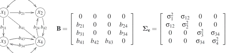
Figure 2: An example of a linear cyclic model with latent variables. A non-zero coefficient b21is represented in the graph by the arc x1→x2. Similarly, the non-zero covariance between disturbances e1 and e2 is represented by the arc x1 ↔x2. In the graph the disturbance term for each individual variable has been omitted for clarity. Note that a pair of opposing directed edges, such as x3→x4 and x3←x4, represents reciprocal causation (feedback relationship) between the variables, whereas a double-headed arrow, such as x3 ↔x4, represents confounding.
2. Model
We start by presenting the basic interpretation of the cyclic model in the passive observational (Section 2.1) and experimental settings (Section 2.2). We establish canonical forms for both the model and the experiments to simplify the presentation of the subsequent theory. We then discuss different stability assumptions to ensure the presence of model equilibria, and show how they relate to the model interpretation and model marginalization (Section 2.3).
2.1 Linear Cyclic Model with Latent Variables
Following the framework presented in Bollen (1989), we consider a general linear structural equa-tion model (SEM) with correlated errors as our underlying data generating model. In such a model the value of each observed variable xj∈
V
( j=1, ...,n) is determined by a linear combination ofthe values of its causal parents xi∈pa(xj)and an additive disturbance (‘noise’) term ej:
xj :=
∑
xi∈pa(xj)bjixi+ej.
Representing all the observed variables as a vector x and the corresponding disturbances as a vector e, these structural equations can be represented by a single matrix equation
x := Bx+e, (1)
where B is the(n×n)-matrix of coefficients bji. A graphical representation of such a causal model
is given by representing any non-zero causal effect bji by an edge xi →xj in the corresponding
graph. An example graph and matrix B are shown in Figure 2.
the corresponding matrix B is lower triangular. When the graph contains directed cycles (feedback loops), such as for the model of Figure 2, then the model is said to be non-recursive or cyclic. In this paper we do not assume a priori that the underlying model is acyclic. In other words, our model family allows for both cyclic and acyclic cases.
While in a ‘fully observed’ SEM the disturbance terms ei would be assumed to be
indepen-dent of each other, we allow for unobserved confounding by modeling arbitrary correlations among the disturbances e1, ...,en. Specifically, denote byµe andΣe the mean vector and the variance-covariance matrix (respectively) of the disturbance vector e. The diagonal elements ofΣerepresent
the variances of the disturbances, while the off-diagonal entries represent the covariances. In the cor-responding graph a non-zero covariance between ei and ejis represented by the double-headed arc
xi↔xj. Notice that in this implicit representation, a latent variable that confounds three observed
variables is represented by three (pairwise) covariances. To keep the notation as simple as possible, we will adopt the assumption standard in the literature that the disturbances have zero mean, that is,
µe=0. In Appendix A we show that it is usually possible to transform the observed data to a form consistent with this assumption. We are thus ready to define the underlying data-generating model:
Definition 1 (Linear Cyclic Model with Latent Variables) A linear cyclic model with latent vari-ables
M
= (B,Σe), is a structural equation model over a set of observed variables x1,· · ·,xn ∈V
of the form of Equation 1, where the disturbance vector e has meanµe=0and an arbitrary
sym-metric positive-definite variance-covariance matrixΣe.
In order to give a fully generative explanation of the relationship between the model parameters and the data, additional constraints on B are needed. Typically, a cyclic model is used to represent a causal process that is collapsed over the time dimension and where it is assumed that the data sample is taken after the causal process has ‘settled down’. The traditional interpretation of non-recursive SEMs assumes that the disturbances represent background conditions that do not change until the system has reached equilibrium and measurements are taken. So for a given set of initial values for the variables x(0), a data vector is generated by drawing one vector of disturbances e from the error distribution and iterating the system
x(t) := Bx(t−1) +e (2)
by adding in the constant (with respect to time) e at every time step until convergence. At time t the vector x thus has the value
x(t) := (B)tx(0) +
t−1
∑
i=0(B)ie.
For x(t)to converge to an equilibrium, the geometric sequence(Bi)i=0...t and the geometric series
∑t−1
i=0Bi must converge as t →∞. For arbitrary x(0) and arbitrary e, a necessary and sufficient condition for this is that the eigenvaluesλk of B satisfy∀k :|λk|<1 (Fisher, 1970). In that case
(B)t →0 and∑t−1
i=0Bi→(I−B)−1as t→∞, so x(t)converges to x = (I−B)−1e,
determined by B and e. Multiple samples of x are obtained by repeating this equilibrating process for different samples of e. Hence, for
M
= (B,Σe)the variance-covariance matrix over the observedvariables is
Cx=E{xxT}= (I−B)−1E{eeT}(I−B)−T = (I−B)−1Σe(I−B)−T. (3) The equilibrium we describe here corresponds to what Lauritzen and Richardson (2002) called a
deterministic equilibrium, since the equilibrium value of x(t)is fully determined given a sample of the disturbances e. Such an equilibrium stands in contrast to a stochastic equilibrium, resulting from a model in which the disturbance term is sampled anew at each time step in the equilibrating process. We briefly return to consider such models in Section 7. We note that if the model happens to be acyclic (i.e., has no feedback loops), the interpretation in terms of a deterministic equilibrium coincides with the standard recursive SEM interpretation, with no adjustments needed.
It is to be expected that in many systems the value of a given variable xiat time t has a non-zero
effect on the value of the same variable at time t+1. (For instance, such systems are obtained when approximating a linear differential equation with a difference equation.) In such a case the coefficient bii(a diagonal element of B) is by definition non-zero, and the model is said to exhibit
a ‘self-loop’ (a directed edge from a node to itself in the graph corresponding to the model). As will be discussed in Section 2.3, such self-loops are inherently unidentifiable from equilibrium data, so there is a need to define a standardized model which abstracts away non-identifiable parameters. For this purpose we introduce the following definition.
Definition 2 (Canonical Model) A linear cyclic model with latent variables(B,Σe)is said to be a
canonical model if it does not contain self-loops (i.e., the diagonal of B is zero).
We will show in Section 2.3 how one can obtain the canonical model that yields in all experiments the same observations at equilibrium as an arbitrary (i.e., including self-loops) linear cyclic model with latent variables.
2.2 Experiments
As noted in the introduction, one of the aims of inferring causal models is the ability to predict how a system will react when it is subject to intervention. One key feature of linear cyclic models with latent variables is that they naturally integrate the representation of experimental manipulations, as discussed in this subsection.
We characterize an experiment
E
k= (J
k,U
k) as a partition of the observed variablesV
(i.e.,J
k∪U
k=V
andJ
k∩U
k=/0) into a setJ
kof intervened variables and a setU
kof passively observedvariables. Note that in this representation, a passive observational data set is a ‘null-experiment’ in which
J
k = /0 andU
k=V
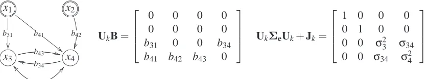
. Following the standard view (Spirtes et al., 2000; Pearl, 2000), weconsider in this paper randomized “surgical” interventions that break all incoming causal influences to the intervened variables by setting the intervened variables to values determined by an exogenous intervention distribution with meanµkcand covariance cov(c) =Σkc. In the graph of the underlying model, this corresponds to cutting all edges into the intervened nodes; see Figure 3 for an example. To simplify notation, we denote by Jkand Uk two(n×n)diagonal ‘indicator matrices’, where
(Jk)ii=1 if and only if xi ∈
J
k, all other entries of Jk are zero, and Uk =I−Jk. The vector c?>=< 89:;76540123x1
b31 b41 F F F F F " " F F F F F ?>=< 89:;76540123x2
b42
?>=<
89:;x3 b43 ++
\ \ σ34 B B ?>=< 89:;x4
b34
k
k
UkB=
0 0 0 0
0 0 0 0
b31 0 0 b34 b41 b42 b43 0
Uk
ΣeUk+Jk=
1 0 0 0
0 1 0 0
0 0 σ23 σ34 0 0 σ34 σ24
Figure 3: Manipulated model corresponding to an intervention on variables x1and x2in the model of Figure 2, that is, the result of an experiment
E
k = (J
k,U
k) withJ
k ={x1,x2} andU
k={x3,x4}.is zero otherwise. The behavior of the model in an experiment
E
k is then given by the structuralequations
x :=UkBx+Uke+c. (4)
For an intervened variable xj∈
J
k, the manipulated model in Equation 4 replaces the originalequa-tion xj :=∑i∈pa(j)bjixi+ej with the equation xj :=cj, while the equations for passively observed
variables xu∈
U
kremain unchanged.Here the intervention vector c is constant throughout the equilibrating process, holding the inter-vened variables fixed at the values sampled from the intervention distribution. A different approach could consider interventions that only “shock” the system initially, and then allow the intervened variables to fluctuate. This would require a different representation and analysis from the one we provide here.
As in the passive observational setting discussed in Section 2.1, we have to ensure that the time series representation of the experimental setting
x(t):=UkBx(t−1) +Uke+c
is guaranteed to converge to an equilibrium as t→∞, where both c and e are time-invariant. We do so by extending the assumption that guarantees convergence in the passive observational setting to
all experimental settings.
Definition 3 (Asymptotic Stability) A linear cyclic model with latent variables(B,Σe)is
asymp-totically stable if and only if for every possible experiment
E
k= (J
k,U
k), the eigenvaluesλi of thematrix UkB satisfy∀i :|λi|<1.
Asymptotic stability implies that in an experiment
E
k= (J
k,U
k)the samples we obtain atequilib-rium are given by x= (I−UkB)−1(Uke+c). Note that the passive observational case is included in
implies that the system under investigation will not break down or explode under any intervention, so the equilibrium distributions are well defined for all circumstances. Obviously, this will not be true for many real feedback systems, and in fact the assumption can be weakened for our purposes. However, as we discuss in more detail in Section 2.3, the assumption of an underlying generating model that satisfies asymptotic stability simplifies the interpretation of our results. For an acyclic model(B,Σe)all eigenvalues of all matrices UkB are zero, so the stability condition is in this case
trivially fulfilled.
In general, experiments can take many forms: Apart from varying several rather than just one variable at the same time, the interventions on the variables can be independent from one another, or correlated, with different means and variances for each intervened variable. To simplify notation for the remainder of this paper, we will adopt a standardized notion of an experiment:
Definition 4 (Canonical Experiment) An experiment
E
k = (J
k,U
k)is said to be a canonicalex-periment if the intervened variables in
J
k are randomized surgically and uncorrelated with thedisturbances and with each other, with zero mean and unit variance.
This notational simplification makes the partition into intervened and passively observed variables the only parameter specifying an experiment, and allows us to derive the theory purely in terms of the covariance matrices Ckx of an experiment. The following lemma shows that we can make the assumption of uncorrelated components of c without loss of generality. First, however, we need one additional piece of notation: For any(n×n)-matrix A, we denote by ASrSc the block of A that remains after deleting the rows corresponding to variables in
V
\S
rand columns corresponding tovariables in
V
\S
c, keeping the order of the remaining rows and columns unchanged.Lemma 5 (Correlated Experiment) If in an experiment
E
k= (J
k,U
k), where interventionvari-ables c are randomized1independently of the disturbances e such that E(c) =µckand cov(c) =Σkc,
a linear cyclic model with latent variables(B,Σe)produces mean ˜µk
xand covariance matrix ˜Ckx,
then in a canonical experiment where intervention variables c are randomized independently of e with E(c) =0 and cov(c) =Jk, the model produces observations with mean and covariance given
by
µkx = 0, (5)
Ckx = C˜k
x−T˜kx(C˜kx)JkJk(T˜
k
x)T+T˜kx(T˜kx)T, (6)
where ˜Tkx= (C˜kx)V Jk((C˜kx)JkJk) −1.
Proof To improve readability, proofs for all lemmas and theorems in this paper are deferred to the appendix.
The lemma shows that whenever in an actual experiment the values given to the intervened variables are not mutually uncorrelated, we can easily convert the estimated mean and covariance matrix to a standardized form that would have been found, had the interventions been uncorrelated with zero mean and unit variance.2 The substantive assumption is that the values of the intervened
1. Randomization implies here that the covariance matrix of the intervention variables cov(cJk) = (Σk
c)JkJkis symmetric
positive-definite.
2. The lemma should come as no surprise to readers familiar with multiple linear regression: The[•,j]-entries of the matrix Tkxare the regression coefficients when xjis regressed over the intervened variables. The regressors do not
variables (the components of c) are uncorrelated with the disturbances (the components of e). This excludes so-called ‘conditional interventions’ where the values of the intervened variables depend on particular observations of other (passively observed) variables in the system. We take this to be an acceptably weak restriction.
Mirroring the derivation in Section 2.1, in a canonical experiment
E
k the mean and covarianceare given by:
µkx = 0, (7)
Ckx = (I−UkB)−1(Jk+UkΣeUk)(I−UkB)−T. (8)
We can now focus on analyzing the covariance matrix obtained from a canonical experiment
E
k = (J
k,U
k) on a canonical model (B,Σe). For notational simplicity we assume without loss of generality that variables x1,· · ·,xj ∈J
k are intervened on and variables xj+1,· · ·,xn∈U
k arepassively observed. The covariance matrix for this experiment then has the block form
Ckx =
I (Tkx)T
Tkx (Ckx)UkUk
, (9)
where
Tkx = (I−BUkUk) −1B
UkJk,
(Ckx)UkUk = (I−BUkUk) −1(B
UkJk(BUkJk)
T+ (Σ
e)UkUk) (I−BUkUk) −T.
The upper left hand block is the identity matrix I, since in a canonical experiment the intervened variables are randomized independently with unit variance. We will consider the more complicated lower right hand block of covariances between the passively observed variables in Section 3.2. The lower left hand block Tkx consists of covariances that represent the so-called experimental effects of the intervened xi∈
J
kon the passively observed xu∈U
k. An experimental effect t(xi xu||J
k)is theoverall causal effect of a variable xion a variable xuin the experiment
E
k= (J
k,U
k); it correspondsto the coefficient of xiwhen xuis regressed on the set of intervened variables in this experiment. If
only variable xi is intervened on in the experiment, then the experimental effect t(xi xu||{xi})is
standardly called the total effect and denoted simply as t(xi xu). If all observed variables except
for xuare intervened on, then an experimental effect is called a direct effect: t(xi xu||
V
\ {xu}) =b(xi→xu) = (B)ui=bui.
The covariance between two variables can be computed by so called ‘trek-rules’. Some form of these rules dates back to the method of path analysis in Wright (1934). In our case, these trek-rules imply that the experimental effect t(xi xu||
J
k)can be expressed as the sum of contributionsby all directed paths starting at xi and ending in xu in the manipulated graph, denoted by the set
P
(xi xu||J
k). The contribution of each path p∈P
(xi xu||J
k) is determined by the product ofthe coefficients bml associated with the edges xl →xm on the path, as formalized by the following
formula
t(xi xu||
J
k) =∑
p∈P(xi xu||Jk)∏
(xl→xm)∈p
bml,
where the product is taken over all edges xl→xmon the path p. The full derivation of this formula
?>=< 89:;x3
0.8
?>=< 89:;x1
−0.8
4
4
−0.7 ''
?>=< 89:;x2 0.9
g
g
?>=< 89:;x1
−1.34
&
&
?>=< 89:;x2 0.9
f
f ?>=<89:;x1
−0.67
&
&
0.5 ++ ?>=<89:;x2 0.45
f
f kk 0.5
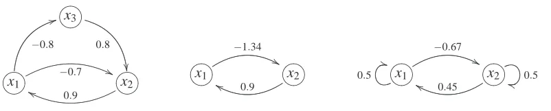
Figure 4: Left: The original asymptotically stable model. Center: The marginalized model that is only weakly stable. Right: A marginalized model with self cycles that is asymptotically stable.
If the model includes cycles, there will be an infinite number of directed paths from one variable to the other. In the example model of Figure 3, the experimental effects can be calculated using the trek-rules as follows:
t(x1 x3||{x1,x2}) = (b31+b41b34)(1+b43b34+ (b43b34)2+· · ·) =
b31+b41b34 1−b43b34
, (10)
t(x1 x4||{x1,x2}) = (b41+b31b43)(1+b43b34+ (b43b34)2+· · ·) =
b41+b31b43 1−b43b34
. (11)
The convergence of the geometric series is guaranteed by the assumption of asymptotic stability for the experiment
J
k={x1,x2}, which ensures that the (only) non-zero eigenvalueλ=b43b34satisfies |λ|<1.Note that the experimental effects are unaffected by the latent confounding. Since the inter-ventions break any incoming arrows on the intervened variables, this independence also follows directly from the graphical d-separation criterion extended to cyclic graphs (Spirtes, 1995): In Fig-ure 3, variables x1 and x3 are not d-connected by any of the undirected paths through the double headed arrows.
2.3 Marginalization
One of the key features of linear structural equation models with correlated errors is that the model family is closed under marginalization. That is, if instead of the original variable set
V
we only have access to a subset ˜V
⊂V
of variables, then if the original model(B,Σe)is in the model family,then the marginalized model (B˜,Σ˜e) over ˜
V
is in the family, too. Any directed paths throughmarginalized variables are transformed into directed edges in ˜B, and any confounding effect of the marginalized variables is integrated into the covariance matrix ˜Σeof the disturbances.
For example, in Figure 4 on the left we show the graph structure and the edge coefficients of an asymptotically stable model(B,Σe)over the variables
V
={x1,x2,x3}. For the purpose ofar-gument, assume that variable x3 is not observed. We thus want to describe a marginalized model (B˜,Σ˜e)over just the variables ˜
V
={x1,x2}. Critically, the two models should produce the sameeffect t(x1 x2||{x1}) =−0.7−0.8·0.8=−1.34 of the original model should equal the corre-sponding experimental effect of the marginalized model. If we do not want to add any additional self-cycles, the only possibility is to set ˜b21=−1.34. Similarly, we set ˜b12=t(x2 x1||{x2}) =0.9. This gives the model of Figure 4 (center).
Note, however, that while the original model was asymptotically stable (as can easily be seen by computing the eigenvalues of B), the marginalized canonical model is not asymptotically stable, as
˜
B has an eigenvalue that is larger than 1 in absolute value. We thus see that when relevant variables are not included in the analysis, asymptotic stability may not hold under marginalization. Fortu-nately, it turns out that for our purposes of identification a much weaker assumption is sufficient. We term this assumption weak stability:
Definition 6 (Weak Stability) A linear cyclic causal model with latent variables(B,Σe)is weakly
stable if and only if for every experiment
E
k= (J
k,U
k), the matrix I−UkB is invertible.Note that the invertibility of matrix I−UkB is equivalent to matrix UkB not having any eigenvalues
equal to exactly 1. (Complex-valued eigenvalues with modulus 1 are allowed as long as the eigen-value in question is not exactly 1+0i.) Any asymptotically stable model is therefore by definition also weakly stable.
We noted earlier that asymptotic stability is an unnecessarily strong assumption for our context. In fact, weak stability is all that is mathematically required for all the theory presented in this article. However, while mathematically expedient, weak stability alone can lead to interpretational ambiguities: Under the time series interpretation of a cyclic model that we presented in Equation 2, a weakly stable model that is not asymptotically stable will fail to have an equilibrium distribution for one or more experiments. While Figure 4 illustrates that asymptotic stability may be lost when marginalizing hidden variables, one cannot in general know whether a learned model that is not asymptotically stable for some experiments corresponds to such an unproblematic case, or whether the underlying system truly is unstable under those experiments.
For the remainder of this article, to ensure a consistent interpretation of any learned model, we assume that there is a true underlying asymptotically stable data generating model, possibly including hidden variables—thereby guaranteeing well-defined equilibrium distributions for all ex-periments. The interpretation of any learned weakly stable model (B,Σe) is then only that the
distribution over the observed variables produced at equilibrium by the true underlying asymptot-ically stable model has mean and covariance as described by Equations 7 and 8.3 All equations derived for asymptotically stable models carry over to weakly stable models.4 In the following two Lemmas, we give the details of how the canonical model over the observed variables is related to the original linear cyclic model in the case of hidden variables and self-cycles (respectively).
The marginalized model of any given linear structural equation model with latent variables can be obtained with the help of the following Lemma.
Lemma 7 (Marginalization) Let(B,Σe)be a weakly stable linear cyclic model over the variables
V
, with latent variables. LetM
⊂V
denote the set of marginalized variables. Then themarginal-3. Alternatively, one could avoid making this assumption of asymptotic stability of the underlying model, but in that case the predictions of the outcomes of experiments must be conditional on the experiments in question resulting in equilibrium distributions.
4. The sums of divergent geometric series can be evaluated by essentially extending the summing formula∑∞i=0bi=1−1b
ized model(B˜,Σ˜e)over variables ˜
V
=V
\M
defined by ˜B = BV˜V˜ +BV M˜ (I−BM M)−1BMV˜, ˜
Σe = (I−B˜)(I−B)−1Σe(I−B)−T˜
VV˜ (I−B˜) T
is also a weakly stable linear cyclic causal model with latent variables. The marginalized covari-ance matrix of the original model and the covaricovari-ance matrix of the marginalized model are equal in any experiments where any subset of the variables in ˜
V
are intervened on.The expressions for ˜B and ˜Σe have simple intuitive explanations. First, the coefficient matrix ˜B
of the marginalized model is given by the existing coefficients between the variables in ˜
V
in the original model plus any paths in the original model from variables in ˜V
through variables inM
and back to variables in ˜V
. Second, the disturbance covariance matrix ˜Σe for the marginalizedmodel is obtained by taking the observed covariances over the variables in ˜
V
and accounting for the causal effects among the variables in ˜V
, so as to ensure that the resulting covariances in the marginal model equal those of the original model in any experiment.In addition to marginalizing unobserved variables, we may be interested in deriving the canon-ical model (i.e., without self-loops) from an arbitrary linear cyclic model with self-loops. This is possible with the following lemma.
Lemma 8 (Self Cycles) Let Uibe an(n×n)-matrix that is all zero except for the element(Ui)ii=1.
For a weakly stable model(B,Σe)containing a self-loop for variable xiwith coefficient bii, we can
define a model without that self-loop given by
˜
B = B− bii 1−bii
Ui(I−B),
˜
Σe = (I+ bii
1−bii
Ui)Σe(I+
bii
1−bii
Ui)T.
The resulting model(B˜,Σ˜e)is also weakly stable and yields the same observations at equilibrium
in all experiments.
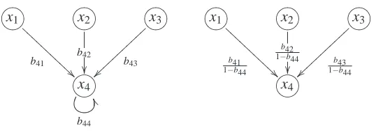
Figure 5 shows explicitly the relation of edge strengths in the two models of the lemma. Since we are only rescaling some of the coefficients, the graph structure of the model stays intact, except for the deleted self-loop. The structure of the covariance matrixΣealso remains unchanged, with only
the ith row and the ith column rescaled. For a model(B,Σe)with several self-loops we can apply
Lemma 8 repeatedly to obtain a model without any self-loops, which is equivalent to the original model in the sense that it yields the same equilibrium data as the original model for all experiments. Note that, as with marginalization, the standardization by removal of self-cycles may produce a canonical model that is only weakly stable, and not asymptotically stable, even if the original model was asymptotically stable.
?>=< 89:;x1
b41 A A A A A A A A A A
A ?>=<89:;x2
b42
?>=< 89:;x3
b43 ~ ~ }}}} }}}} }}} ?>=< 89:;x4
b44
U
U
?>=< 89:;x1
b41 1−b44 AAA
A A A A A A A
A ?>=<89:;x2 b42 1−b44
?>=< 89:;x3
b43 1−b44
~ ~ }}}} }}}} }}} ?>=< 89:;x4
Figure 5: Perturbation of coefficients from a model with self-loops (on the left) to a model without self-loops (on the right). The two models are indistinguishable from equilibrium data.
3. Identifiability
The full characterization of the model under passive observational and experimental circumstances now allows us to specify conditions (on the set of experiments) that are sufficient (Section 3.1) and necessary (Section 3.2) to identify the model parameters. Throughout, for purposes of full identi-fication (uniqueness of the solution) and notational simplicity, we assume that in each experiment we observe the covariance matrix in the infinite sample limit as described by Equation 8, and that both the underlying model and all experiments are canonical. For reasons discussed in the previous section we also assume that there is an underlying generating model that is asymptotically stable, even though the marginalized parts of the model we observe may only be weakly stable. Readers who are primarily interested in the learning algorithm we have developed can skip to Section 4 and return to the identifiability conditions of this section when required.
3.1 Sufficiency
Going back to our four variable example in Figure 3, in which x1 and x2 are subject to interven-tion, we already derived in Equations 10 and 11 the experimental effects t(x1 x3||{x1,x2}) and t(x1 x4||{x1,x2})using the trek-rules. Taken together, these equations imply the following
t(x1 x3||{x1,x2}) = b31+t(x1 x4||{x1,x2})b34 (12) = t(x1 x3||{x1,x2,x4}) +t(x1 x4||{x1,x2})t(x4 x3||{x1,x2,x4}).
Note that Equation 12 relates the experimental effects of intervening on{x1,x2}to the experimental effects of intervening on{x1,x2,x4}. It shows that the experimental effect t(x1 x3||{x1,x2})can be calculated by separating the single path not going through x4 (with contribution b31) from the remaining paths that all go through x4. The last edge on these paths is always x4→x3. The total contribution of the paths through x4is therefore the product t(x1 x4||{x1,x2})b34.
linear constraints on the (unknown) direct effects bji. Thus, if we had a set of experiments that
sup-plies constraints that would be sufficient for us to solve for all the direct effects, then we would again be able to identify the B-matrix. In either case, the question crucial for identifiability is: Which sets of experiments produce experimental effects that are sufficient to identify the model? Unsurpris-ingly, the answer is the same for both cases. For reasons of simplicity, we present the identifiability proof in this section in terms of the first approach. We use the second approach, involving a system of linear constraints, for the learning algorithm in Section 4.
The example in Equation 12 can be generalized in the following way: As stated earlier, for an asymptotically stable model, the experimental effect t(xi xu||
J
k)of xi ∈J
k on xu∈U
k inex-periment
E
k= (J
k,U
k) is the sum-product of coefficients on all directed paths from xi to xu. Wecan calculate the sum-product in two parts with respect to an observed variable xj ∈
U
k. First weconsider all the paths that do not go through xj. The sum-product of all those paths is equal to
the experimental effect t(xi xu||
J
k∪ {xj}), since all paths through xj are intercepted byaddition-ally intervening on xj. Second, the remaining paths are all of the form xi x˜j xu, where ˜xjis the
last occurrence of xj on the path (recall that paths may contain cycles, so there may be multiple
occurrences of xj on the path). The sum-product of coefficients on all subpaths xi x˜j is given
by t(xi xj||
J
k)and the sum-product of coefficients on all subpaths ˜xj xuis t(xj xu||J
k∪ {xj}).Taking all combinations of subpaths xi x˜j and ˜xj xu, we obtain the contribution of all the paths
through xj as the product t(xi xj||
J
k)t(xj xu||J
k∪ {xj}). We thus obtaint(xi xu||
J
k) = t(xi xu||J
k∪ {xj}) +t(xi xj||J
k)t(xj xu||J
k∪ {xj}). (13)This equation is derived formally in Appendix F, where it is also shown that it holds for all weakly stable models (not only asymptotically stable models).
We now show that equations of the above type from two different experiments can be combined to determine the experimental effects of a novel third experiment. Consider for example the model in Figure 2 over variables
V
={x1,x2,x3,x4}. Say, we have conducted two single-intervention exper-imentsE
1= (J
1,U
1) = ({x1},{x2,x3,x4})andE
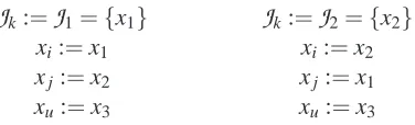
2= ({x2},{x1,x3,x4}). By making the following substitutions in Equation 13 for each experiment, respectively,J
k:=J
1={x1} xi:=x1 xj:=x2 xu:=x3J
k:=J
2={x2} xi:=x2 xj:=x1 xu:=x3we get two equations relating the experimental effects in the original two experiments to some experimental effects of the union experiment
E
3= ({x1,x2},{x3,x4})(we denote it as the “union” experiment becauseJ
3=J
1∪J
2):
1 t(x1 x2||{x1}) t(x2 x1)||{x2}) 1
t(x1 x3||{x1,x2}) t(x2 x3||{x1,x2})
=
t(x1 x3||{x1}) t(x2 x3||{x2})
.
following lemma shows that the matrix is invertible when the weak stability condition holds, and that in general, from experimental effects observed in two experiments, we can always estimate the experimental effects in their union and in their intersection experiments.
Lemma 9 (Union/Intersection Experiment) For a weakly stable canonical model the experimen-tal effects in two experiments
E
k= (J
k,U
k)andE
l= (J
l,U
l)determine the experimental effects in• the union experiment
E
k∪l= (J
k∪J
l,U
k∩U
l), and• the intersection experiment
E
k∩l= (J
k∩J
l,U
k∪U
l).Since there are no experimental effects in experiments intervening on /0 or
V
, the experimental effects are considered to be determined trivially in those cases. In the case of union experiments, also the full covariance matrix Ckx∪l of the experiment can be determined. For intersection experiments, Ckx∩l can be fully determined if passive observational data is available (see Appendix J).In a canonical model the coefficients b(•→xu) on the arcs into variable xu (the direct effects
of the other variables on that variable) are equal to the experimental effects when intervening on everything except xu, that is, b(•→xu) =t(• xu||
V
\ {xu}). So in order to determine particulardirect effects, it is sufficient to ensure that a given set of experiments provides the basis to apply Lemma 9 repeatedly so as to obtain the experimental effects of the experiments that intervene on all but one variable. In our example with four variables, we can first use Lemma 9 to calculate the experimental effects when intervening on{x1} ∪ {x2}={x1,x2}(as suggested above), and given a further experiment that intervenes only on x4, we can then determine the experimental effects of an experiment intervening on{x1,x2} ∪ {x4}={x1,x2,x4}. The experimental effects we obtain constitute the direct effects b(•→x3). Hence, if single-intervention experiments are available for each variable it is easy to see that all direct effects of the model are identified using the lemma.
What then is the general condition on the set of experiments such that we can derive all possible direct effects by iteratively applying Lemma 9? It turns out that we can determine all direct effects if the following pair condition is satisfied for all ordered pairs of variables.
Definition 10 (Pair Condition) A set of experiments {
E
k}k=1,...,K satisfies the pair condition foran ordered pair of variables(xi,xu)∈
V
×V
(with xi6=xu) whenever there is an experimentE
k=(
J
k,U
k)in{E
k}k=1,...,Ksuch that xi∈J
k(xiis intervened on) and xu∈U
k(xuis passively observed).It is not difficult to see that the pair condition holding for all ordered pairs of variables is suffi-cient to identify B. Consider one variable xu. From a set of experiments satisfying the pair condition
for all ordered pairs, we can find for all xi6=xu an experiment satisfying the pair condition for the
pair(xi,xu). We refer to such an experiment as ˜
E
i= (J
˜i,U
˜i)in the following. Now, by iterativelyusing Lemma 9, we can determine the experimental effects in the union experiment ˜
E
∪= (J
˜∪,U
˜∪) of experiments{E
˜i}i6=u, where variables in set ˜J
∪=Si6=uJ
˜i are intervened on. Each xi wasinter-vened on at least in one experiment, thus∀i6=u : xi∈
J
˜∪. Variable xu was passively observed ineach experiment, thus xu∈/
J
˜∪. The experimental effects of this union experiment intervening on ˜J
∪=V
\ {xu}are thus the direct effects b(•→xu). Repeating the same procedure for each xu∈V
Thus, if the pair condition is satisfied for all ordered pairs, we can determine all elements of B, and only the covariance matrixΣe of the disturbances remains to be determined. The passive
observational data covariance matrix C0x can be estimated from a null-experiment
E
0= (/0,V
). Given B and C0xwe can solve forΣeusing Equation 3:Σe = (I−B)C0
x(I−B)T. (14)
If there is no null-experiment, then the block(Σe)U
k,Uk of the covariance matrix can instead be determined from the covariance matrix in any experiment
E
k= (J
k,U
k)using Equation 8:(Σe)U
kUk = [(I−UkB)C
k
x(I−UkB)T]UkUk. (15) Consequently, given B, we can determine(Σe)i j=σi j if the following covariance condition is met.
Definition 11 (Covariance Condition) A set of experiments{
E
k}k=1,...,K satisfies the covariancecondition for an unordered pair of variables{xi,xj} ⊆
V
whenever there is an experimentE
k=(
J
k,U
k)in(E
k)k=1,...,Ksuch that xi∈U
kand xj∈U
k, that is, both variables are passively observed.Similarly to the pair condition, if we know B, and if the covariance condition is satisfied for all pairs of variables, we can identify all covariances inΣe. Notice that the variances(Σe)iican be
determined since the assumption includes that each variable xi must be passively observed at least
in one experiment.
Putting the results together we get a sufficient identifiability condition for a canonical model:
Theorem 12 (Identifiability–Sufficiency) Given canonical experiments{
E
k}k=1,...,Ka weaklysta-ble canonical model(B,Σe)over the variables
V
is identifiable if the set of experiments satisfies thepair condition for each ordered pair of variables(xi,xj)∈
V
×V
(with xi6=xj) and the covariancecondition for each unordered pair of variables{xi,xj} ⊆
V
.The identifiability condition is satisfied for our four-variable case in Figure 2 by, for exam-ple, a set of experiments intervening on {x1,x2},{x2,x4},{x1,x4} and{x3}. Obviously, a full set of single-intervention experiments or a full set of all-but-one experiments together with a passive observational data set would also do. We return to this issue in Section 4.2.
3.2 Necessity
To show that the conditions of Theorem 12 are not only sufficient but in fact also necessary for identifiability, we consider what happens when the pair condition or the covariance condition is not satisfied for some variable pair. Since the covariance condition only ensures the identifiability of
Σewhen B is already identified, we start with the more fundamental pair condition.
Consider the two models in Figure 6. The models differ in their parameters, and even in their structure, yet produce the same observations in all experiments that do not satisfy the pair condition for the (ordered) pair (x2,x4). That is, for any experiment (including a passive observation), for which it is not the case that x2∈
J
k and x4∈U
k, the two models are indistinguishable, despite the?>=<
89:;x1 b21 //
b31 b41 E E E E E E E " " E E E E E E E w
w σ12 ((?>=<89:;
x2
b42
?>=<
89:;x3 b43 ++?>=<89:;x4
b34
k
k
?>=<
89:;x1 b21 //
b31
b41+b42b21
&
&
w
w σ12 ((
j j b42σ12 ?>=< 89:;x2
Y
Y
b42σ2 2
?>=<
89:;x3 b43 ++?>=<89:;x4
b34
k
k
Figure 6: Underdetermination of the model. On the left: the data generating model(B,Σe). On the
right: a model(B˜,Σ˜e)producing the same observations in all experiments not satisfying the pair condition for the ordered pair(x2,x4).
(x2,x4), its effect can be accounted for elsewhere in the right model, for example, the effect of the missing path x1→x2→x4 is accounted for in the model on the right by the perturbed coefficient b41+b42b21on the arc x1→x4.
The ˜B-matrix for the model on the right was constructed from the one on the left by perturbing the coefficient b42 corresponding to the pair(x2,x4), for which the pair condition is not satisfied. The perturbation corresponds to settingδ:=−b42in the following lemma.
Lemma 13 (Perturbation of B) Let B be the coefficient matrix of a weakly stable canonical model over
V
and let{E
k}k=1,...,Kbe a set of experiments on B that does not satisfy the pair condition forsome pair(xi,xj). Denote the sets
K
=V
\ {xi,xj}andL
={xi,xj}. Then a model with coefficientmatrix ˜B defined by ˜
BK V =BK V, B˜LL=
0 bi j
bji+δ 0
, B˜LK = (I−B˜LL)(I−BLL)−1BLK
will produce the same experimental effects as B for any experiment that does not satisfy the pair condition for the pair(xi,xj). The free parameterδmust be chosen such that ˜B is weakly stable.
Lemma 13 shows that if the pair condition is not satisfied for the pair(xi,xj), then bji cannot be
identified on the basis of the measured experimental effects. As in our example, it is generally the case that forδ6=0 the models B and ˜B will produce different experimental effects in any experiment that satisfies the pair condition for the pair(xi,xj). The choice ofδis not crucial, since most choices
will produce a weakly stable perturbed model.
To see the effect of the perturbation more clearly, we can write it explicitly as follows:
∀l6= j,∀k : ˜blk=blk, (no changes to any edges that do not end in xj)
˜bji=bji+δ, (perturb the direct effect of xion xjbyδ)
˜bj j=0, (no self-loop at xj)
∀k∈ {/ i,j}: ˜bjk=bjk−δ
bik+bi jbjk
1−bi jbji
. (needed adjustments to incoming arcs to xj)
The above form makes it clear that if the pair condition is not satisfied for the pair (xi,xj), in
identifiability of coefficient bji we must have the pair condition satisfied for all pairs (•,xj). In
Figure 6 the coefficient b42 is unidentified because the pair condition for the pair (x2,x4) is not satisfied. But as a result, b41 is also unidentified. Nevertheless, in this particular example, the coefficient b43happens to be identified, because of the structure of the graph.
If the pair condition is not satisfied for several pairs, then Lemma 13 can be applied iteratively for each missing pair to arrive at a model with different coefficients, that produces the same experi-mental effects as the original for all experiments not satisfying the pairs in question. Each missing pair adds an additional degree of freedom to the system.
We emphasize that Lemma 13 only ensures that the experimental effects of the original and perturbed model are the same. However, the following lemma shows that the covariance matrix of disturbances can always be perturbed such that the two models become completely indistinguishable for any experiment that does not satisfy the pair condition for some pair(xi,xj), as was the case in
Figure 6.
Lemma 14 (Perturbation ofΣe) Let the true model generating the data be (B,Σe). For each
of the experiments{
E
k}k=1,...,K, let the obtained data covariance matrix be Ckx. If there exists acoefficient matrix ˜B6=B such that for all{
E
k}k=1,...,K and all xi∈J
k and xj∈U
k it produces thesame experimental effects t(xi xj||
J
k), then the model(B˜,Σ˜e)with ˜Σe= (I−B˜)(I−B)−1Σe(I− B)−T(I−B˜)T produces data covariance matrices ˜Ckx=Ckxfor all k=1, ...,K.
Lemma 14, in combination with Lemma 13, shows that for identifiability the pair condition must be satisfied for all pairs. If the pair condition is not satisfied for some pair, then an alternative model (distinct from the true underlying model) can be constructed (using the two lemmas) which produces the exact same covariance matrices Ckxfor all the available experiments. In Figure 6, the effect of the missing link x2→x4is imitated by the additional covariance b42σ22between e2and e4 and by the covariance b42σ12between e1and e4.
The result implies that identifying the coefficient matrix B exclusively on the basis of constraints based on experimental effects already fully exploits the information summarized by the second order statistics. The covariances between the passively observed variables (corresponding to the lower right hand block in Equation 9) do not provide any further information. We thus obtain the result:
Theorem 15 (Completeness) Given the covariance matrices in a set of experiments{
E
k}k=1,...,Kover the variables in
V
, all coefficients b(xi→xj)of a weakly stable canonical model are identifiedif and only if the pair condition is satisfied for all ordered pairs of variables with respect to these experiments.
Intuitively, the covariances between the passively observed variables do not help in identifying the coefficients B because they also depend on the unknownsΣe, and the additional unknowns swamp
the gains of the additional covariance measures.
If B is known or the pair condition is satisfied for all pairs, but the covariance condition is not satisfied for a pair {xi,xj}, then in general the covariance σi j cannot be identified: In all the
manipulated graphs of the experiments the arc xi↔xj is cut, and thusσi jdoes not affect the data in
any way. It follows that the covariance condition is necessary as well. However, unlike for the pair condition, not satisfying the covariance condition for some pair does not affect the identifiability of any of the other covariances.
condition for all pairs is sufficient for model identifiability. Theorem 15 shows that the coefficients cannot be identified if the pair condition is not satisfied for all pairs of variables, and in the previous paragraph we showed that satisfying the covariance condition for all pairs is necessary to identify all covariances and variances of the disturbances. This yields the following main result.
Corollary 16 (Model Identifiability) The parameters of a weakly stable canonical model(B,Σe)
over the variables in
V
can be identified if and only if the set of experiments{E
k}k=1,...,K satisfiesthe pair condition for all ordered pairs (xi,xj)∈
V
×V
(such that xi 6=xj) and the covariancecondition for all unordered pairs{xi,xj} ⊆
V
.Finally, note that all of our identifiability results and our learning algorithm (Section 4) are solely based on second-order statistics of the data and the stated model space assumptions. No additional background knowledge is included. When the data are multivariate Gaussian, these statistics exhaust the information available, and hence our identifiability conditions are (at least) in this case necessary.
4. Learning Method
In this section, we present an algorithm, termed LLC, for inferring a linear cyclic model with latent variables, provided finite sample data from a set of experiments over the given variable set. Although Lemma 9 (Union/Intersection Experiment) naturally suggests a procedure for model discovery given a set of canonical experiments that satisfy the conditions of Corollary 16 (Model Identifiability), we will pursue a slightly different route in this section. It allows us to not only identify the model when possible, but can also provide a more intuitive representation of the (common) situation when the true model is either over- or underdetermined by the given set of experiments. As before, we will continue to assume that we are considering a set of canonical experiments on a weakly stable canonical model (Definitions 2, 4 and 6). From the discussion in Section 2 it should now be clear that this assumption can be made essentially without loss of generality: Any asymptotically stable model can be converted into a weakly stable canonical model and any experiment can be redescribed as a canonical experiment, as long as the interventions in the original experiment were independent of the disturbances. As presented here, the basic LLC algorithm provides only estimates of the values of all the edge coefficients in B, as well as estimates of the variances and covariances among the disturbances inΣe. We later discuss how to obtain error estimates for the parameters and how
to adapt the basic algorithm to different learning tasks such as structure discovery.
4.1 LLC Algorithm
To illustrate the derivation of the algorithm, we again start with Equation 12, which was derived from the experiment that intervenes on x1and x2in Figure 3,
t(x1 x3||{x1,x2}) = b31+t(x1 x4||{x1,x2})b34.
This provides a linear constraint of the measured experimental effects t(x1 xj||{x1,x2}) on the unknown direct effects b31 and b34 into x3. In general, the experimental effects observed in an experiment
E
k= (J
k,U
k)can be used to provide linear constraints on the unknown direct effectsthat, like Equation 12, have the form
t(xi xu||