Towards More Efficient SPSD Matrix Approximation
and CUR Matrix Decomposition
Shusen Wang [email protected]
Department of Statistics
University of California at Berkeley Berkeley, CA 94720, USA
Zhihua Zhang [email protected] School of Mathematical Sciences
Peking University Beijing 100871, China
Tong Zhang [email protected]
Department of Statistics Rutgers University
Piscataway, New Jersey 08854, USA
Editor:Gert Lanckriet
Abstract
Symmetric positive semi-definite (SPSD) matrix approximation methods have been extensively used to speed up large-scale eigenvalue computation and kernel learning methods. The standard sketch based method, which we call the prototype model, produces
relatively accurate approximations, but is inefficient on large square matrices. The Nystr¨om
method is highly efficient, but can only achieve low accuracy. In this paper we propose a
novel model that we call the fast SPSD matrix approximation model. The fast model is
nearly as efficient as the Nystr¨om method and as accurate as the prototype model. We
show that the fast model can potentially solve eigenvalue problems and kernel learning
problems in linear time with respect to the matrix size n to achieve 1 + relative-error,
whereas both the prototype model and the Nystr¨om method cost at least quadratic time
to attain comparable error bound. Empirical comparisons among the prototype model,
the Nystr¨om method, and our fast model demonstrate the superiority of the fast model.
We also contribute new understandings of the Nystr¨om method. The Nystr¨om method is
a special instance of our fast model and is approximation to the prototype model. Our technique can be straightforwardly applied to make the CUR matrix decomposition more efficiently computed without much affecting the accuracy.
Keywords: Kernel approximation, matrix factorization, the Nystr¨om method, CUR matrix decomposition
1. Introduction
(Woodruff, 2014), the machine learning community (Mahoney, 2011), and the numerical linear algebra community (Halko et al., 2011).
In machine learning, many graph analysis techniques and kernel methods require expensive matrix computations on symmetric matrices. The truncated eigenvalue decom-position (that is to find a few eigenvectors corresponding to the greatest eigenvalues) is widely used in graph analysis such as spectral clustering, link prediction in social networks (Shin et al., 2012), graph matching (Patro and Kingsford, 2012), etc. Kernel methods (Sch¨olkopf and Smola, 2002) such as kernel PCA and manifold learning require the truncated eigenvalue decomposition. Some other kernel methods such as Gaussian process regression/classification require solving n×n matrix inversion, where n is the number of training samples. The rank k (k n) truncated eigenvalue decomposition (k-eigenvalue decomposition for short) of ann×nmatrix costs time ˜O(n2k)1; the matrix inversion costs time O(n3). Thus, the standard matrix computation approaches are infeasible when n is large.
For kernel methods, we are typically given n data samples of dimension d, while the
n×n kernel matrix Kis unknown beforehand and should be computed. This adds to the additional O(n2d) time cost. When n and d are both large, computing the kernel matrix
is prohibitively expensive. Thus, a good kernel approximation method should avoid the computation of the entire kernel matrix.
Typical SPSD matrix approximation methods speed up matrix computation by effi-ciently forming a low-rank decomposition K ≈ CUCT where C ∈ Rn×c is a sketch of
K (e.g., randomly sampled c columns of K) and U ∈ Rc×c can be computed in different
ways. With such a low-rank approximation at hand, it takes onlyO(nc2) additional time to approximately compute the rankk(k≤c) eigenvalue decomposition or the matrix inversion. Therefore, ifCand Uare obtained in linear time (w.r.t.n) andcis independent of n, then the aforementioned eigenvalue decomposition and matrix inversion can be approximately solved in linear time.
The Nystr¨om method is perhaps the most widely used kernel approximation method. LetP be ann×csketching matrix such as uniform sampling (Williams and Seeger, 2001; Gittens, 2011), adaptive sampling (Kumar et al., 2012), leverage score sampling (Gittens and Mahoney, 2016), etc. The Nystr¨om method computes C by C= KP∈Rn×c and U
by U= (PTC)†∈Rc×c. This way of computing U is very efficient, but it incurs relatively
large approximation error even ifCis a good sketch ofK. As a result, the Nystr¨om method is reported to have low approximation accuracy in real-world applications (Dai et al., 2014; Hsieh et al., 2014; Si et al., 2014b). In fact, the Nystr¨om is impossible to attain 1 +
bound relative to kK−Kkk2F unless c ≥ Ω
p
nk/
(Wang and Zhang, 2013). Here Kk
denotes the best rank-kapproximation ofK. The requirement thatcgrows at least linearly with √n is a very pessimistic result. It implies that in order to attain 1 + relative-error bound, the time cost of the Nystr¨om method is of order nc2 = Ω(n2k/) for solving the
k-eigenvalue decomposition or matrix inversion, which is quadratic inn. Therefore, under the 1 +relative-error requirement, the Nystr¨om method is not a linear time method.
The main reason for the low accuracy of the Nystr¨om method is due to the way that the
U matrix is calculated. In fact, much higher accuracy can be obtained if U is calculated
by solving the minimization problem minUkK−CUCTk2F, which is a standard way to
approximate symmetric matrices (Halko et al., 2011; Gittens and Mahoney, 2016; Wang and Zhang, 2013; Wang et al., 2016). This is the randomized SVD for symmetric matrices (Halko et al., 2011). Wang et al. (2016) called this approach the prototype model and provided an algorithm that samples c = O(k/) columns of K to form C such that minUkK−
CUCTk2
F ≤(1 +)kK−Kkk2F. Unlike the Nystr¨om method, the prototype model does not
requirec to grow with n. The downside of the prototype model is the high computational cost. It requires the full observation ofKand O(n2c) time to compute U. Therefore when applied to kernel approximation, the time cost cannot be less thanO(n2d+n2c). To reduce the computational cost, this paper considers the problem of efficient calculation ofU with fixed Cwhile achieving an accuracy comparable to the prototype model.
More specifically, the key question we try to answer in this paper can be described as follows.
Question 1 For any fixed n×n symmetric matrix K, target rank k, and parameter γ, assume that
A1 We are given a sketch matrixC∈Rn×c ofK, which is obtained in time Time(C); A2 The matrixC is a good sketch ofK in thatminUkK−CUCTkF2 ≤(1 +γ)kK−Kkk2F.
Then we would like to know whether for an arbitrary , it is possible to compute Cand ˜
U such that the following two requirements are satisfied: R1 The matrixU˜ has the following error bound:
kK−CUC˜ Tk2F ≤(1 +)(1 +γ)kK−Kkk2F.
R2 The procedure of computing C and U˜ and approximately solving the aforementioned k -eigenvalue decomposition or the matrix inversion run in time O n· poly(k, γ−1, −1)
+
Time(C).
Unfortunately, the following theorem shows that neither the Nystr¨om method nor the prototype model enjoys such desirable properties. We prove the theorem in Appendix B.
Theorem 1 Neither the Nystr¨om method nor the prototype model satisfies the two requirements in Question 1. To make requirement R1 hold, both the Nystr¨om method and the prototype model cost time no less than O n2·poly(k, γ−1, −1)
+Time(C) which is at least quadratic in n.
In this paper we give an affirmative answer to the above question. In particular, it has the following consequences. First, the overall approximation has high accuracy in the sense thatkK−CUC˜ Tk2
F is comparable to minUkK−CUCTk2F, and is thereby comparable to
the best rankkapproximation. Second, withCat hand, the matrix ˜Uis obtained efficiently (linear in n). Third, with Cand ˜U at hand, it takes extra time which is also linear in n
to compute the aforementioned eigenvalue decomposition or linear system. Therefore, with a good C, we can use linear time to obtain desired U matrix such that the accuracy is comparable to the best possible low-rank approximation.
matrices. Given anym×nfixed matrixA, the CUR matrix decomposition selectsccolumns ofAto formC∈Rm×candrrows ofAto formR∈Rr×n, and computes matrixU ∈Rc×r such thatkA−CURk2
F is small. Traditionally, it costs time
O(mn·min{c, r})
to compute the optimalU? =C†AR†(Stewart, 1999; Wang and Zhang, 2013; Boutsidis and Woodruff, 2014). How to efficiently compute a high-qualityU matrix for CUR is unsolved.
1.1 Main Results
This work is motivated by an intrinsic connection between the Nystr¨om method and the prototype model. Based on a generalization of this observation, we propose the fast SPSD matrix approximation model for approximating any symmetric matrix. We show that the fast model satisfies the requirements in Question 1. Given n data points of dimension d, the fast model computes C and Ufast and approximately solves the truncated eigenvalue decomposition or matrix inversion in time
O nc3/+nc2d/
+ Time(C).
Here Time(C) is defined in Question 1.
The fast SPSD matrix approximation model achieves the desired properties in Question 1 by solving minUkK−CUCTkF approximately rather than exactly while ensuring
kK−CUfastCTk2
F ≤(1 +) min
U kK−CUC
Tk2 F.
The time complexity for computing Ufast is linear in n, which is far less than the time complexity O(n2c) of the prototype model. Our method also avoids computing the entire kernel matrixK; instead, it computes a block ofKof size
√
nc ×
√
nc
, which is substantially
smaller than n×n. The lower bound in Theorem 7 indicates that the √n factor here is optimal, but the dependence onc and are suboptimal and can be potentially improved.
This paper provides a new perspective on the Nystr¨om method. We show that, as well as our fast model, the Nystr¨om method is approximate solution to the problem minUkCUCT−
Kk2
F. Unfortunately, the approximation is so rough that the quality of the Nystr¨om method
is low.
Our method can also be applied to improve the CUR matrix decomposition of the general matrices which are not necessarily square. Given any matrices A∈Rm×n,C∈Rm×c, and
R∈Rr×n, it costs time O(mn·min{c, r}) to compute the matrixU =C†AR†. Applying our technique, the time cost drops to only
O cr−1·min{m, n} ·min{c, r} ,
while the approximation quality is nearly the same.
1.2 Paper Organization
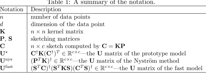
Table 1: A summary of the notation.
Notation Description
n number of data points
d dimension of the data point
K n×nkernel matrix
P,S sketching matrices
C n×csketch computed byC=KP
U? C†K(C†)T ∈
Rc×c—theUmatrix of the prototype model
Unys (PTK)†∈
Rc×c—theUmatrix of the Nystr¨om method
Ufast (STC)†(STKS)(CTS)† ∈Rc×c—theUmatrix of the fast model
approximation. Section 4 describes our fast model and analyze the time complexity and error bound. Section 5 applies the technique of the fast model to compute the CUR matrix decomposition more efficiently. Section 6 conducts empirical comparisons to show the effect of the U matrix. The proofs of the theorems are in the appendix.
2. Notation
The notation used in this paper are defined as follows. Let [n] = {1, . . . , n}, In be the
n×n identity matrix, and 1n be the n×1 vector of all ones. We let x ∈ y ±z denote
y−z ≤ x ≤ y+z. For an m×n matrix A = [Aij], we let ai: be its i-th row, a:j be its
j-th column, nnz(A) be the number of nonzero entries of A, kAkF = (Pi,jA2ij)1/2 be its
Frobenius norm, and kAk2 = maxx6=0kAxk2/kxk2 be its spectral norm.
Let ρ = rank(A). The condensed singular value decomposition (SVD) of A is defined as
A = UΣVT =
ρ
X
i=1
σiuiviT
where σ1,· · · , σr are the positive singular values in the descending order. We also use
σi(A) to denote the i-th largest singular value of A. Unless otherwise specified, in this
paper “SVD” means the condensed SVD. Let Ak = Pki=1σiuiviT be the top k principal
components of A for any positive integer k less than ρ. In fact, Ak is the closest to A
among all the rankk matrices. LetA†=VΣ−1UT be theMoore-Penrose inverseof A.
Assume that ρ = rank(A) < n. The column leverage scores of A are li = kvi:k22 for
i = 1 to n. Obviously, l1 +· · ·+ln = ρ. The column coherence is defined by ν(A) = n
ρmaxj∈[n]kvj:k 2
2. Ifρ= rank(A)< m, the row leverage scores and coherence are similarly
defined. The row leverage scores are ku1:k2
2,· · · ,kum:k22 and the row coherence is µ(A) = m
ρ maxi∈[m]kui:k22.
We also list some frequently used notation in Table 1. Given the decomposition ˜K=
3. Related Work
In Section 3.1 we introduce matrix sketching. In Section 3.2 we describe two SPSD matrix approximation methods.
3.1 Matrix Sketching
Popular matrix sketching methods include uniform sampling, leverage score sampling (Drineas et al., 2006, 2008; Woodruff, 2014), Gaussian projection (Johnson and Linden-strauss, 1984), subsampled randomized Hadamard transform (SRHT) (Drineas et al., 2011; Lu et al., 2013; Tropp, 2011), count sketch (Charikar et al., 2004; Clarkson and Woodruff, 2013; Meng and Mahoney, 2013; Nelson and Nguyˆen, 2013; Pham and Pagh, 2013; Thorup and Zhang, 2012; Weinberger et al., 2009), etc.
3.1.1 Column Sampling
Let p1,· · · , pn ∈ (0,1) with
Pn
i=1pi = 1 be the sampling probabilities. Let each integer
in [n] be independently sampled with probabilities sp1,· · · , spn, where s ∈ [n] is integer.
Assume that ˜s integers are sampled from [n]. Let i1,· · · , i˜s denote the selected integers,
and let E[˜s] =s. We scale each selected column by √1
spi1,
· · · ,√1
spi˜s, respectively. Uniform
sampling means that the sampling probabilities are p1 = · · · = pn = 1n. Leverage score
sampling means that the sampling probabilities are proportional to the leverage scores
l1,· · · , ln of a certain matrix.
We can equivalently characterize column selection by the matrixS∈Rn×s˜. Each column of S has exactly one nonzero entry; let (ij, j) be the position of the nonzero entry in the
j-th column forj ∈[˜s]. For j= 1 to ˜s, we set
Sij,j=
1
√
spij
. (1)
The expectation E[˜s] equals to s, and ˜s = Θ(s) with high probability. For the sake of simplicity and clarity, in the rest of this paper we will not distinguish ˜sand s.
3.1.2 Random Projection
LetG∈Rn×sbe a standard Gaussian matrix, namely each entry is sampled independently
fromN(0,1). The matrixS= √1
sGis a Gaussian projection matrix. Gaussian projection is
also well known as the Johnson-Lindenstrauss (JL) transform (Johnson and Lindenstrauss, 1984); its theoretical property is well established. It takesO(mns) time to applyS∈Rn×s
to any m×n dense matrix, which makes Gaussian projection inefficient.
The subsampled randomized Hadamard transform (SRHT) is usually a more efficient alternative of Gaussian projection. Let Hn ∈ Rn×n be the Walsh-Hadamard matrix with +1 and−1 entries,D∈Rn×nbe a diagonal matrix with diagonal entries sampled uniformly from {+1,−1}, andP∈Rn×s be the uniform sampling matrix defined above. The matrix S = √1
nDHnP∈R
n×s is an SRHT matrix, and it can be applied to any m×n matrix in
O(mnlogs) time.
matrix S ∈ Rn×s can be applied to any matrix A in O(nnz(A)) time where nnz denotes
the number of non-zero entries. The readers can refer to (Woodruff, 2014) for detailed descriptions of count sketch.
3.1.3 Theories
The following lemma shows important properties of the matrix sketching methods. In the lemma, leverage score sampling means that the sampling probabilities are proportional to the row leverage scores of the column orthogonal matrix U ∈ Rn×k. (Here U is different
from the notation elsewhere in the paper.) We prove the lemma in Appendix C.
Lemma 2 Let U∈Rn×k be any fixed matrix with orthonormal columns andB∈Rn×d be any fixed matrix. LetS∈Rn×s be any sketching matrix considered in this section; the order
of s (with theO-notation omitted) is listed in Table 2. Then
P
n
UTSSTU−Ik
2 ≥η
o
≤ δ1 (Property 1),
P
n
UTB−UTSSTB
2
F ≥kBk 2 F
o
≤ δ2 (Property 2),
P
n
UTB−UTSSTB
2 2 ≥
0kBk2 2+
0
kkBk
2 F
o
≤ δ3 (Property 3).
Table 2: The leverage score sampling is w.r.t. the row leverage scores of U. For uniform sampling, the notationµ(U)∈[1, n] is the row coherence ofU.
Sketching Property 1 Property 2 Property 3 Leverage Sampling ηk2 logδk
1
k
δ2 —
Uniform Sampling µ(ηU2)klogδk 1
µ(U)k
δ2 —
Gaussian Projection k+log(1/δ1)
η2 δk2 10 k+ logkδd
3
SRHT k+logη2 nlogδk 1
k+logn δ2
1
0 k+ logkδnd 1
logδd
3
Count Sketch δk2
1η2
k
δ2 —
Property 1 is known as the subspace embedding property (Woodruff, 2014). It shows that all the singular values ofSTUare close to one. Properties 2 and 3 show that sketching preserves the multiplication of a row orthogonal matrix and an arbitrary matrix.
3.2 SPSD Matrix Approximation Models
We first describe the prototype model and the Nystr¨om method, which are most relevant to this work. We then introduce several other SPSD matrix approximation methods.
3.2.1 Most Relevant Work
Given an n×n matrix K and an n×c sketching matrix P, we let C = KP and W =
PTC=PTKP. The prototype model (Wang and Zhang, 2013) is defined by
˜
Kprotoc , CU?CT = CC†K(C†)TCT, (2) and the Nystr¨om method is defined by
˜
Knysc , CUnysCT = CW†CT
= C PTC† PTKP CTP†CT. (3)
The only difference between the two models is theirUmatrices, and the difference leads to big difference in their approximation accuracies. Wang and Zhang (2013) provided a lower error bound of the Nystr¨om method, which shows that no algorithm can select less than Ω(pnk/) columns ofK to formCsuch that
kK−CUnysCTk2F ≤(1 +)kK−Kkk2F.
In contrast, the prototype model can attain the 1 +relative-error bound withc=O(k/) (Wang et al., 2016), which is optimal up to a constant factor.
While we have mainly discussed the time complexity of kernel approximation in the previous sections, the memory cost is often a more important issue in large scale problems due to the limitation of computer memory. The Nystr¨om method and the prototype model require O(nc) memory to hold Cand U to approximately solve the aforementioned eigenvalue decomposition or the linear system.2 Therefore, we hope to make c as small as possible while achieving a low approximation error. There are two elements: (1) a good sketch C=KP, and (2) a high-qualityU matrix. We focus on the latter in this paper.
3.2.2 Less Relevant Work
We note that there are many other kernel approximation approaches in the literature. However, these approaches do not directly address the issue we consider here, so they are complementary to our work. These studies are either less effective or inherently rely on the Nystr¨om method.
The Nystr¨om-like models such as MEKA (Si et al., 2014a) and the ensemble Nystr¨om method (Kumar et al., 2012) are reported to significantly outperform the Nystr¨om method in terms of approximation accuracy, but their key components are still the Nystr¨om method and the component can be replaced by any other methods such as the method studied in this work. The spectral shifting Nystr¨om method (Wang et al., 2014) also outperforms the
2. The memory costs of the prototype model isO(nc+nd) rather thanO(n2). This is because we can hold
then×ddata matrix and thec×nmatrixC† in memory, compute a small block ofKeach time, and
Nystr¨om method in certain situations, but the spectral shifting strategy can be used for any other kernel approximation models beyond the prototype model. We do not compare with these methods in this paper because MEKA, the ensemble Nystr¨om method, and the spectral shifting Nystr¨om method can all be improved if we replace the underlying Nystr¨om method or the prototype model by the new method developed here.
The column-based low-rank approximation model (Kumar et al., 2009) is another SPSD matrix approximation approach different from the Nystr¨om-like methods. Let P ∈ Rn×c
be any sketching matrix and C = KP. The column-based model approximates K by
C(CTC)−1/2CT = (CCT)1/2. Equivalently, it approximatesK2 by
KTK ≈ CCT = KTPPTK.
From Lemma 2 we can see that it is a typical sketch based approximation to the matrix multiplication. Unfortunately, the approximate matrix multiplication is effective only when
Khas much more rows than columns, which is not true for the kernel matrix. The column-based model does not have good error bound and is not empirically as good as the Nystr¨om method (Kumar et al., 2009).
The random feature mapping (Rahimi and Recht, 2007) is a family of kernel approxima-tion methods. Each random feature mapping method is applicable to certain kernel rather than arbitrary SPSD matrix. Furthermore, they are known to be noticeably less effective than the Nystr¨om method (Yang et al., 2012).
4. The Fast SPSD Matrix Approximation Model
In Section 4.1 we present the motivation behind the fast model. In Section 4.2 we provide an alternative perspective on our fast model and the Nystr¨om method by formulating them as approximate solutions to an optimization problem. In Section 4.3 we analyze the error bound of the fast model. Theorem 3 is the main theorem, which shows that in terms of the Frobenius norm approximation, the fast model is almost as good as the prototype model. In Section 4.4 we describe the implementation of the fast model and analyze the time complexity. In Section 4.5 we give some implementation details that help to improve the approximation quality. In Section 4.6 we show that our fast model exactly recoversK
under certain conditions, and we provide a lower error bound of the fast model.
4.1 Motivation
Let P ∈ Rn×c be sketching matrix and C = KP ∈ Rn×c. The fast SPSD matrix approximation model is defined by
˜
Kfastc,s , C STC† STKS CTS†CT,
whereS is n×ssketching matrix.
From (2) and (3) we can see that the Nystr¨om method is a special case of the fast model where S is defined as Pand that the prototype model is a special case where S is defined asIn.
The fast model allows us to trade off the accuracy and the computational cost—larger
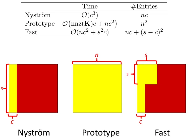
Table 3: Summary of the time cost of the models for computing the U matrices and the number of entries ofKrequired to be observed in order to compute theUmatrices. As for the fast model, assume that S is column selection matrix. The notation is defined previously in Table 1.
Time #Entries
Nystr¨om O(c3) nc
Prototype O nnz(K)c+nc2 n2
Fast O(nc2+s2c) nc+ (s−c)2
Nyström
Prototype
Fast
s n
c c
s
n
Figure 1: The yellow blocksdenote the submatrices of Kthat must be seen by the kernel approximation models. The Nystr¨om method computes an n×c block of K, provided that P is column selection matrix; the prototype model computes the entiren×nmatrixK; the fast model computes ann×cblock and an (s−c)×(s−c) block of K (due to the symmetry of K), provided that P and S are column selection matrices.
sacrifices too much accuracy, whereas setting s as large as n is unnecessarily expensive. Later on, we will show that s = O(cpn/) n is a good choice. The setting s n
makes the fast model much cheaper to compute than the prototype model. When applied to kernel methods, the fast model avoids computing the entire kernel matrix. We summarize the time complexities of the three matrix approximation methods in Table 3; the middle column lists the time cost for computing theU matrices given Cand K; the right column lists the number of entry ofKwhich much be observed. We show a very intuitive comparison in Figure 1.
4.2 Optimization Perspective
With the sketch C = KP ∈ Rn×c at hand, we want to find the U matrix such that
tight:
U? = argmin U
CUCT −K
2 F = C
†K(C†)T. (4)
This is the prototype model. Since solving this system is time expensive, we propose to draw a sketching matrix S∈Rn×s and solve the following problem instead:
Ufast = argmin U
ST(CUCT −K)S
2 F
= argmin
U
(STC)U(STC)T −STKS
2 F
= (STC)†(STKS)(CTS)†, (5)
which results in the fast model. Similar ideas have been exploited to efficiently solve the least squares regression problem (Drineas et al., 2006, 2011; Clarkson and Woodruff, 2013), but their analysis can not be directly applied to the more complicated system (5).
This approximate linear system interpretation offers a new perspective on the Nystr¨om method. The U matrix of the Nystr¨om method is in fact an approximate solution to the problem minUkCUCT −Kk2F. The Nystr¨om method uses S=Pas the sketching matrix,
which leads to the solution
Unys = argmin U
PT(CUCT −K)P
2
F = (P
TKP)† = W†.
4.3 Error Analysis
LetUfast correspond to the fast model (5). Any of the five sketching methods in Lemma 2 can be used to compute Ufast, although column selection is more useful than random
projection in this application. In the following we show that Ufast is nearly as good as
U? in terms of the objective function value. The proof is in Appendix D.
Theorem 3 (Main Result) Let Kbe any n×n fixed symmetric matrix, Cbe anyn×c
fixed matrix,kc= rank(C), andUfast be thec×cmatrix defined in (5). LetS∈Rn×s be any of the five sketching matrices defined in Table 4. Assume that −1 =o(n) or −1 =o(n/c). The inequality
K−CUfastCT
2
F ≤ (1 +) minU
K−CUCT
2
F (6)
holds with probability at least 0.8.
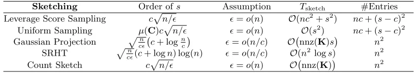
In the theorem, Gaussian projection and SRHT require smaller sketch size than the other three methods. It is because Gaussian projection and SRHT enjoys all of Properties 1, 2, 3 in Lemma 2, whereas leverage score sampling, uniform sampling, and count sketch does not enjoy Property 3.
Remark 4 Wang et al. (2016) showed that there exists an algorithm (though not linear-time algorithm) attaining the error bound
K−CC†K(C†)TCT
2
F ≤ (1 +)
K−Kk
Table 4: Leverage score sampling means sampling according to the row leverage scores of
C. For uniform sampling, the parameterµ(C)∈[1, n] is the row coherence of C.
Sketching Order ofs Assumption Tsketch #Entries
Leverage Score Sampling cp
n/ =o(n) O(nc2+s2) nc+ (s−c)2
Uniform Sampling µ(C)cp
n/ =o(n) O(s2) nc+ (s−c)2
Gaussian Projection pn
c c+ log
n c
=o(n/c) O nnz(K)s
n2
SRHT pn
c(c+ logn) log(n) =o(n/c) O(n
2 logs) n2
Count Sketch cp
n/ =o(n) O nnz(K)
n2
Algorithm 1 The Fast SPSD Matrix Approximation Model.
1: Input: ann×nsymmetric matrix Kand the number of selected columns or target dimension
of projectionc (< n).
2: Sketching: C=KPusing an arbitraryn×c sketching matrixP(not studied in this work);
3: Optional: replaceC by any orthonormal bases of the columns ofC;
4: Compute anothern×ssketching matrixS, e.g. the leverage score sampling in Algorithm 2;
5: Compute the sketches STC∈Rs×c andSTKS∈Rs×s;
6: ComputeUfast= (STC)†(STKS)(CTS)†∈Rc×c;
7: Output: CandUfast such thatK≈CUfastCT.
with high probability by sampling c = O(k/) columns of K to form C. Let C ∈ Rn×c
be formed by this algorithm and S ∈ Rn×s be the leverage score sampling matrix. With
c=O(k/) and s= ˜O(n1/2k−3/2), the fast model satisfies
K−CUfastCT
2
F ≤ (1 +)
K−Kk
2 F
with high probability.
4.4 Algorithm and Time Complexity
We describe the whole procedure of the fast model in Algorithm 1, where S∈Rn×scan be
one of the five sketching matrices described in Table 4. Given Cand (the whole or a part of)K, it takes time
O s2c+Tsketch
to compute Ufast, where Tsketch is the time cost of forming the sketches STC and STKS
and is described in Table 4. In Table 4 we also show the number of entries ofK that must be observed. From Table 4 we can see that column selection is much more efficient than random projection, and column selection does not require the full observation ofK.
Algorithm 2 The Leverage Score Sampling Algorithm.
1: Input: ann×cmatrixC, an integers.
2: Compute the condensed SVD of C (by discarding the zero singular values) to obtain the
orthonormal basesUC∈Rn×ρ, whereρ= rank(C)≤c;
3: Compute the sampling probabilities pi=s`i/ρ, where`i=keTi UCk22 is thei-th leverage score;
4: InitializeSto be an matrices of sizen×0;
5: fori= 1 tondo
6: With probabilitypi, add
q c
s`ieito be a new column ofS, whereeiis thei-th standard basis;
7: end for
8: Output: S, whose expected number of columns iss.
4.5 Implementation Details
In practice, the approximation accuracy and numerical stability can be significantly improved by the following techniques and tricks.
If P and S are both random sampling matrices, then empirically speaking, enforcing
P ⊂ S significantly improves the approximation accuracy. Here P and S are the subsets of [n] selected by Pand S, respectively. Instead of directly samplingsindices from [n] by Algorithm 2, it is better to sample s indices from [n]\ P to form S0 and let S = S0 ∪ P. In this way, s+c columns are sampled. Whether the requirement P ⊂ S improves the accuracy is unknown to us.
Corollary 5 Theorem 3 still holds when we restrict P ⊂ S.
Proof Letp1,· · ·, pnbe the original sampling probabilities without the restriction P ⊂ S.
We define the modified sampling probabilities by
˜
pi =
1 ifi∈ P;
pi otherwise .
The column sampling with restriction P ⊂ S amounts to sampling columns according to ˜
p1,· · ·,p˜n. Since ˜pi ≥pi for alli∈[n], it follows from Remark 14 that the error bound will
not get worse if pi is replaced by ˜pi.
If S is the leverage score sampling matrix, we find it better not to scale the entries of
S, although the scaling is necessary for theoretical analysis. According to our observation, the scaling sometimes makes the approximation numerically unstable.
4.6 Additional Properties
WhenKis a low-rank matrix, the Nystr¨om method and the prototype model are guaranteed to exactly recoverK(Kumar et al., 2009; Talwalkar and Rostamizadeh, 2010; Wang et al., 2016). We show in the following theorem that the fast model has the same property. We prove the theorem in Appendix E.
In the following we establish a lower error bound of the fast model, which implies that to attain the 1 + Frobenius norm bound relative to the best rank k approximation, the fast model must satisfy
c≥Ω k/ and s≥Ω pnk/.
Notice that the theorem only holds for column selection matrices P and S. We prove the theorem in Appendix F.
Theorem 7 (Lower Bound) Let P ∈ Rn×c and S ∈ Rn×s be any two column selection matrices such that P ⊂ S ⊂ [n], where P and S are the index sets formed by P and S, respectively. There exists ann×n symmetric matrix K such that
kK−K˜fastc,s k2F
kK−Kkk2F
≥ n−c
n−k
1 +2k
c
+ n−s
n−k
k(n−s)
s2 , (7)
where k is arbitrary positive integer smaller than n, C=KP∈Rn×c, and
˜
Kfastc,s = C(STC)†(STKS)(CTS)†CT
is the fast model.
Interestingly, Theorem 7 matches the lower bounds of the Nystr¨om method and the prototype model. When s=c, the right-hand side of (7) becomes Ω(1 +kn/c2), which is the lower error bound of the Nystr¨om method given by Wang and Zhang (2013). When
s=n, the right-hand side of (7) becomes Ω(1 +k/c), which is the lower error bound of the prototype model given by Wang et al. (2016).
5. Extension to CUR Matrix Decomposition
In Section 5.1 we describe the CUR matrix decomposition and establish an improved error bound of CUR in Theorem 8. In Section 5.2 we use sketching to more efficiently compute theU matrix of CUR. Theorem 8 and Theorem 9 together show that our fast CUR method satisfies 1 + error bound relative to the best rank k approximation. In Section 5.3 we provide empirical results to intuitively illustrate the effectiveness of our fast CUR. In Section 5.4 we discuss the application of our results beyond the CUR decomposition.
5.1 The CUR Matrix Decomposition
Given any m×n matrix A, the CUR matrix decomposition is computed by selecting c
columns ofA to formC∈Rm×cand r rows ofA to formR∈Rr×n and computing the U matrix such that kA−CURk2
F is small. CUR preserves the sparsity and non-negativity
properties ofA; it is thus more attractive than SVD in certain applications (Mahoney and Drineas, 2009). In addition, with the CUR ofA at hand, the truncated SVD of A can be very efficiently computed.
A standard way to finding the U matrix is by minimizingkA−CURk2
F to obtain the
optimalU matrix
U? = argmin U
which has been used by Stewart (1999); Wang and Zhang (2013); Boutsidis and Woodruff (2014). This approach costs timeO(mc2+nr2) to compute the Moore-Penrose inverse and
O(mn·min{c, r}) to compute the matrix product. Therefore, even ifCandRare uniformly sampled fromA, the time cost of CUR is O(mn·min{c, r}).
At present the strongest theoretical guarantee is by Boutsidis and Woodruff (2014). They use the adaptive sampling algorithm to select c = O(k/) column and r = O(k/) rows to form C and R, respectively, and form U? =C†AR†. The approximation error is bounded by
kA−CU?Rk2F ≤ (1 +)kA−Akk2F.
This result matches the theoretical lower bound up to a constant factor. Therefore this CUR algorithm is near optimal. We establish in Theorem 8 an improved error bound of the adaptive sampling based CUR algorithm, and the constants in the theorem are better than the those in (Boutsidis and Woodruff, 2014). Theorem 8 is obtained by following the idea of Boutsidis and Woodruff (2014) and slightly changing the proof of Wang and Zhang (2013). The proof is in Appendix G.
Theorem 8 Let A be any given m×n matrix, k be any positive integer less than m and
n, and∈(0,1)be an arbitrary error parameter. LetC∈Rm×c and R∈
Rr×n be columns and rows of A selected by the near-optimal column selection algorithm of Boutsidis et al. (2014). Whenc andr are both greater than 4k−1 1 +o(1)
, the following inequality holds:
EA−CC†AR†Rk2F ≤ (1 +)kA−Akk2F,
where the expectation is taken w.r.t. the random column and row selection.
5.2 Fast CUR Decomposition
Analogous to the fast SPSD matrix approximation model, the CUR decomposition can be sped up while preserving its accuracy. Let SC ∈ Rm×sc and SR ∈ Rn×sr be any sketching matrices satisfying the approximate matrix multiplication properties. We propose to computeU more efficiently by
˜
U = argmin U
kSTCASR−(SCTC)U(RSR)k2F
= (STCC)†
| {z }
c×sc
(STCASR)
| {z }
sc×sr
(RSR)†
| {z }
sr×r
, (9)
which costs time
O(srr2+scc2+scsr·min{c, r}) +Tsketch,
where Tsketch denotes the time for forming the sketches STCASR, STCC, and RSR. As for
Gaussian projection, SRHT, and count sketch,Tsketchare respectivelyO nnz(A) min{sc, sr}
,
O mnlog(min{sc, sr})
, and O nnz(A). As for leverage score sampling and uniform sampling, Tsketch are respectively O(mc2+nr2+scsr) and O(scsr). Forming the sketches
by column selection is more efficient than by random projection.
The following theorem shows that when sc and sr are sufficiently large, ˜U is nearly as
good as the best possible U matrix. In the theorem, leverage score sampling means that
SC andSRsample columns according to the row leverage scores ofCand RT, respectively.
Theorem 9 Let A ∈Rm×n, C∈
Rm×c, R∈Rr×n be any fixed matrices with c n and
r m. Let q = min{m, n} and q˜= min{m/c, n/r}. The sketching matrices SC ∈ Rm×sc and SR∈Rn×sr are described in Table 5. Assume that −1 =o(q) or −1 =o(˜q), as shown in the table. The matrix U˜ is defined in (9). Then the inequality
kA−CUR˜ k2F ≤ (1 +) min
U kA−CURk
2 F
holds with probability at least 0.7.
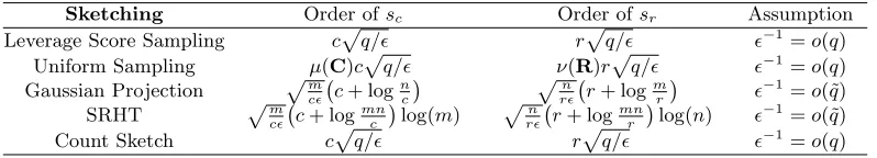
Table 5: Leverage score sampling means sampling according to the row leverage scores of
C and the column leverage scores of R, respectively. For uniform sampling, the parameter µ(C) is the row coherence of Cand ν(R) is the column coherence of
R.
Sketching Order ofsc Order ofsr Assumption
Leverage Score Sampling cp
q/ rp
q/ −1=o(q)
Uniform Sampling µ(C)cp
q/ ν(R)rp
q/ −1=o(q)
Gaussian Projection pm
c c+ log
n c
pn
r r+ log
m r
−1=o(˜q)
SRHT pm
c c+ log
mn c
log(m) pn
r r+ log
mn r
log(n) −1=o(˜q)
Count Sketch cp
q/ rp
q/ −1=o(q)
As for leverage score sampling, uniform sampling, and count sketch, the sketch sizes
sc = O(c
p
q/) and sr = O(r
p
q/) suffice, where q = min{m, n}. As for Gaussian projection and SRHT, much smaller sketch sizes are required: sc = O˜(
p
mc/) and
sr = ˜O(
p
nr/) suffice. However, these random projection methods are inefficient choices in this application and only have theoretical interest. Only column sampling methods have linear time complexities. IfSC and SR are leverage score sampling matrices (according to
the row leverage scores ofCandRT, respectively), it follows from Theorem 9 that ˜Uwith 1 +bound can be computed in time
O srr2+scc2+scsr·min{c, r}
+Tsketch = O cr−1·min{m, n} ·min{c, r}
,
which is linear in O(min{m, n}).
5.3 Empirical Comparisons
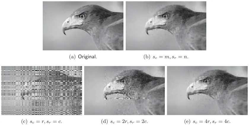
To intuitively demonstrate the effectiveness of our method, we conduct a simple experiment on a 1920×1168 natural image obtained from the internet. We first uniformly sample
c= 100 columns to form Cand r = 100 rows to formR, and then compute theU matrix by varyingscand sr. We show the image ˜A=CURin Figure 2.
Figure 2(b) is obtained by computing the U matrix according to (8), which is the best possible result whenCandRare fixed. TheUmatrix of Figure 2(c) is computed according to Drineas et al. (2008):
wherePC and PRare column selection matrices such thatC=APC andR=PTRA. This
is equivalently to (9) by setting SC = PR and SR =PC. Obviously, this setting leads to
very poor quality. In Figures 2(c) and (d) the sketching matrices SC and SR are uniform
sampling matrices. The figures show that when sc and sr are moderately greater than r
and c, respectively, the approximation quality is significantly improved. Especially, when
sc = 4r and sr = 4c, the approximation quality is nearly as good as using the optimal U
matrix defined in (8).
(a)Original. (b)sc=m, sr=n.
(c)sc=r, sr=c. (d) sc= 2r, sr= 2c. (e)sc= 4r, sr= 4c.
Figure 2: (a): the original 1920×1168 image. (b) to (e): CUR decomposition withc=r= 100 and different settings ofsc and sr.
5.4 Discussions
We note that we are not the first to use row and column sampling to solve the CUR problem more efficiently, though we are the first to provide rigorous error analysis. Previous work has exploited similar ideas as heuristics to speed up computation and to avoid visiting every entry ofA. For example, the MEKA method (Si et al., 2014a) partitions the kernel matrix
Kintob2 blocks K(i,j) (i= 1,· · · , b andj = 1,· · · , b), and requires solving L(i,j) = argmin
L
W(i)LW(j)
T
−K(i,j)
2 F
Table 6: A summary of the datasets for kernel approximation. Dataset Letters PenDigit Cpusmall Mushrooms WineQuality
#Instance 15,000 10,992 8,192 8,124 4,898
#Attribute 16 16 12 112 12
σ(whenη= 0.90) 0.400 0.101 0.075 1.141 0.314
σ(whenη= 0.99) 0.590 0.178 0.180 1.960 0.486
our analysis answers why this approach is correct. This also implies that our algorithms and analysis may have broad applications and impacts beyond the CUR decomposition and SPSD matrix approximation.
0 0.1 0.2 0.3 0.4 0.32
0.34 0.36 0.38 0.4
Error Ratio
s/n
(a)Letters,η= 0.9.
0 0.1 0.2 0.3 0.4 0.04
0.045 0.05 0.055 0.06
Error Ratio
s/n
(b) Letters,η= 0.99.
0 0.1 0.2 0.3 0.4 0.28
0.3 0.32 0.34 0.36 0.38
Error Ratio
s/n
(c)PenDigit,η= 0.9.
0 0.1 0.2 0.3 0.4 0.05
0.06 0.07 0.08 0.09
Error Ratio
s/n
(d) PenDigit,η= 0.99.
0 0.1 0.2 0.3 0.4 0.32
0.34 0.36 0.38 0.4
Error Ratio
s/n
(e)Cpusmall,η= 0.9.
0 0.1 0.2 0.3 0.4 0.032
0.034 0.036 0.038 0.04 0.042 0.044 0.046
Error Ratio
s/n
(f)Cpusmall,η= 0.99.
0 0.1 0.2 0.3 0.4 0.26
0.28 0.3 0.32 0.34 0.36
Error Ratio
s/n
(g)Mushrooms,η= 0.9.
0 0.1 0.2 0.3 0.4 0.045
0.05 0.055 0.06 0.065 0.07 0.075
Error Ratio
s/n
(h)Mushrooms,η= 0.99.
0 0.1 0.2 0.3 0.4 0.24
0.26 0.28 0.3 0.32 0.34
Error Ratio
s/n
(i)Wine,η= 0.9.
0 0.1 0.2 0.3 0.4 0.03
0.035 0.04 0.045 0.05 0.055
Error Ratio
s/n
(j)Wine,η= 0.99.
Fast (leverage) Fast (uniform) Nystrom Prototype
(k)Legend.
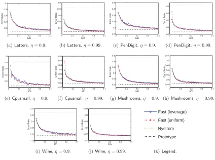
Figure 3: The plot of sn against the approximation errorkK−CUCTk2
F/kKk2F, where C
0 0.1 0.2 0.3 0.4 0.22 0.23 0.24 0.25 0.26 0.27 0.28 0.29 Error Ratio s/n
(a)Letters,η= 0.9.
0 0.1 0.2 0.3 0.4 0.03 0.035 0.04 0.045 0.05 Error Ratio s/n
(b) Letters,η= 0.99.
0 0.1 0.2 0.3 0.4 0.24 0.26 0.28 0.3 0.32 0.34 Error Ratio s/n
(c)PenDigit,η= 0.9.
0 0.1 0.2 0.3 0.4 0.035 0.04 0.045 0.05 0.055 0.06 Error Ratio s/n
(d) PenDigit,η= 0.99.
0 0.1 0.2 0.3 0.4 0.195 0.2 0.205 0.21 0.215 0.22 0.225 0.23 Error Ratio s/n
(e)Cpusmall,η= 0.9.
0 0.1 0.2 0.3 0.4 0.028 0.03 0.032 0.034 0.036 Error Ratio s/n
(f)Cpusmall,η= 0.99.
0 0.1 0.2 0.3 0.4 0.26 0.28 0.3 0.32 0.34 0.36 Error Ratio s/n
(g)Mushrooms,η= 0.9.
0 0.1 0.2 0.3 0.4 0.04 0.045 0.05 0.055 0.06 0.065 Error Ratio s/n
(h)Mushrooms,η= 0.99.
0 0.1 0.2 0.3 0.4 0.22 0.24 0.26 0.28 0.3 0.32 Error Ratio s/n
(i)Wine,η= 0.9.
0 0.1 0.2 0.3 0.4 0.03 0.032 0.034 0.036 0.038 0.04 0.042 0.044 Error Ratio s/n
(j)Wine,η= 0.99.
Fast (leverage) Fast (uniform) Nystrom Prototype
(k)Legend.
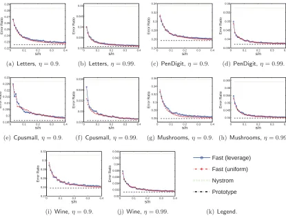
Figure 4: The plot of sn against the approximation errorkK−CUCTk2
F/kKk2F, where C
contains c = dn/100e column of K ∈ Rn×n selected by the uniform+adaptive2
sampling algorithm (Wang et al., 2016).
6. Experiments
In this section we conduct several sets of illustrative experiments to show the effect of the
U matrix. We compare the three methods with different settings of c and s. We do not compare with other kernel approximation methods for the reasons stated in Section 3.2.2.
6.1 Setup
LetX= [x1, . . . ,xn] be the d×ndata matrix, andKbe the RBF kernel matrix with each
entry computed byKij = exp −
kxi−xjk22 2σ2
where σ is the scaling parameter. When comparing the kernel approximation error kK−CUCTk2
F, we set the scaling
parameterσ in the following way. We letk=dn/100eand define
η = kKkk
2 F kKk2
F
=
Pk
i=1σ 2 i(K)
Pn
which indicate the importance of the top one percent singular values of K. In general η
grows withσ. We set σ such that η= 0.9 or 0.99.
All the methods are implemented in MATLAB and run on a laptop with Intel i5 2.5GHz CUP and 8GB RAM. To compare the running time, we set MATLAB in the single thread mode.
6.2 Kernel Approximation Accuracy
We conduct experiments on several datasets available at the LIBSVM site. The datasets are summarized in Table 6. In this set of experiments, we study the effect of the U matrices. We use two methods to form C ∈ Rn×c: uniform sampling and the uniform+adaptive2
sampling (Wang et al., 2016); we fix c=dn/100e. For our fast model, we use two kinds of sketching matricesS∈Rn×s: uniform sampling and leverage score sampling; we varysfrom
2c to 40c. We plot ns against the approximation error kK−CUCTk2
F/kKk2F in Figures 3
and 4. The Nystr¨om method and the prototype model are included for comparison. Figures 3 and 4 show that the fast SPSD matrix approximation model is significantly better than the Nystr¨om method when sis slightly larger than c, e.g., s= 2c. Recall that the prototype model is a special case of the fast model wheres=n. We can see that the fast model is nearly as accurate as the prototype model when sis far smaller than n, e.g.,
s= 0.2n.
The results also show that using uniform sampling and leverage score sampling to generate S does not make much difference. Thus, in practice, one can simply compute
S by uniform sampling.
By comparing the results in Figures 3 and 4, we can see that computing C by uniform+adaptive2 sampling is substantially better than uniform sampling. However, adaptive sampling requires the full observation of K; thus with uniform+adaptive2 sampling, our fast model does not have much advantage over the prototype model in terms of time efficiency. Our main focus of this work is the U matrix, so in the rest of the experiments we simply use uniform sampling to computeC.
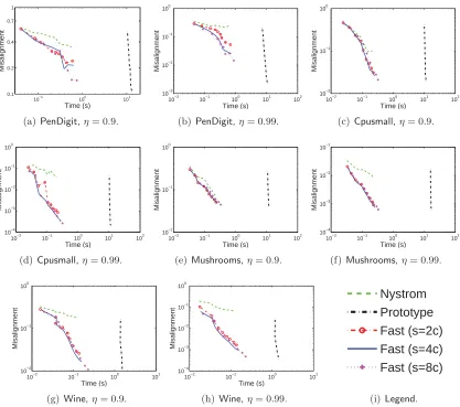
6.3 Approximate Kernel Principal Component Analysis
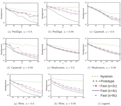
We apply the three methods to approximately compute kernel principal component analysis (KPCA), and contrast with the exact solution. The experiment setting follows Zhang and Kwok (2010). We fix k and vary c. For our fast model, we set s = 2c, 4c, or 8c. Since computing S by uniform sampling or leverage score sampling yields the same empirical performance, we use only uniform sampling. Let CUCT be the low-rank approximation formed by the three methods. Let ˜VΛ˜V˜T be thek-eigenvalue decomposition ofCUCT.
6.3.1 Quality of the Approximate Eigenvectors
Let UK,k ∈ Rn×k contain the top k eigenvectors of K. In the first set of experiments, we measure the distance between UK,k and the approximate eigenvectors ˜Vby
Misalignment = 1
k
UK,k−V˜V˜TUK,k
2
F (∈ [0,1]). (10)
10−1 100 101 0.1
0.2 0.4 0.7 1
Misalignment
Time (s)
(a)PenDigit,η= 0.9.
10−2 10−1 100 101 102 10−3
10−2 10−1 100
Misalignment
Time (s)
(b)PenDigit,η= 0.99.
10−2 10−1 100 101 102 10−2
10−1 100
Misalignment
Time (s)
(c) Cpusmall,η= 0.9.
10−2 10−1 100 101 102 10−4
10−3 10−2 10−1 100
Misalignment
Time (s)
(d)Cpusmall,η= 0.99.
10−2 10−1 100 101 102 10−2
10−1 100
Misalignment
Time (s)
(e) Mushrooms,η= 0.9.
10−2 10−1 100 101 102 10−4
10−3 10−2 10−1
Misalignment
Time (s)
(f) Mushrooms,η= 0.99.
10−2 10−1 100 101 10−2
10−1 100
Misalignment
Time (s)
(g)Wine,η= 0.9.
10−2 10−1 100 101 10−4
10−3 10−2 10−1 100
Misalignment
Time (s)
(h)Wine,η= 0.99.
Nystrom Prototype Fast (s=2c) Fast (s=4c) Fast (s=8c)
(i)Legend.
Figure 5: The plot of (log-scale) elapsed time against the (log-scale) misalignment defined in (10).
We conduct experiments on the datasets summarized in Table 6. We record the elapsed time of the entire procedure—computing (part of) the kernel matrix, computing C and
U by the kernel approximation methods, computing the k-eigenvalue decomposition of
CUCT. We plot the elapsed time against the misalignment defined in Figure 5. Results on the Letters dataset are not reported because the exact k-eigenvalue decomposition on MATLAB ran out of memory, making it impossible to calculate the misalignment.
At the end of Section 3.2.1 we have mentioned the importance of memory cost of the kernel approximation methods and that all three compared methods cost O(nc+nd) memory. Since n and d are fixed, we plot c against the misalignment in Figure 6 to show the memory efficiency.
30 60 90 120 150 10−1
100
Misalignment
c
(a)PenDigit,η= 0.9.
30 60 90 120 150
10−3 10−2 10−1 100
Misalignment
c
(b)PenDigit,η= 0.99.
30 60 90 120 150
10−2 10−1 100
Misalignment
c
(c) Cpusmall,η= 0.9.
30 60 90 120 150
10−4 10−3 10−2 10−1 100
Misalignment
c
(d)Cpusmall,η= 0.99.
40 60 80 100 120 140 10−2
10−1 100
Misalignment
c
(e) Mushrooms,η= 0.9.
40 60 80 100 120 140 10−4
10−3 10−2 10−1
Misalignment
c
(f) Mushrooms,η= 0.99.
40 60 80 100 120 140 10−2
10−1 100
Misalignment
c
(g)Wine,η= 0.9.
30 60 90 120 150
10−4 10−3 10−2 10−1 100
Misalignment
c
(h)Wine,η= 0.99.
Nystrom Prototype Fast (s=2c) Fast (s=4c) Fast (s=8c)
(i)Legend.
Figure 6: The plot ofc against the (log-scale) misalignment defined in (10).
Table 7: A summary of the datasets for clustering and classification.
Dataset MNIST Pendigit USPS Mushrooms Gisette DNA
#Instance 60,000 10,992 9,298 8,124 7,000 2,000
#Attribute 780 16 256 112 5,000 180
#Class 10 10 10 2 2 3
Scaling Parameterσ 10 0.7 15 3 50 4
experiment also shows that with fixedc, the fast model is nearly as accuracy as the prototype model whens= 8cn.
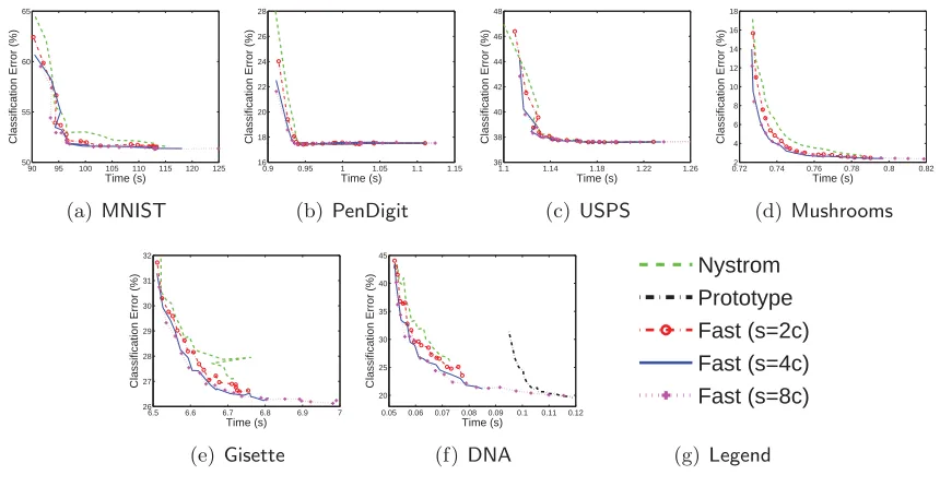
6.3.2 Quality of the Generalization
0 20 40 60 80 100 50
55 60 65
Classification Error (%)
c
(a) MNIST
0 20 40 60 80 100 16 18 20 22 24 26 28
Classification Error (%)
c
(b) PenDigit
0 20 40 60 80 100 38 40 42 44 46 48
Classification Error (%)
c
(c)USPS
0 20 40 60 80 100 2 4 6 8 10 12 14 16 18
Classification Error (%)
c
(d) Mushrooms
0 20 40 60 80 100 25 26 27 28 29 30 31 32
Classification Error (%)
c
(e)Gisette
0 20 40 60 80 100 15 20 25 30 35 40 45
Classification Error (%)
c (f)DNA Nystrom Prototype Fast (s=2c) Fast (s=4c) Fast (s=8c) (g) Legend
Figure 7: The plot of c against the classification error. Herek= 3.
90 95 100 105 110 115 120 125 50
55 60 65
Classification Error (%)
Time (s)
(a) MNIST
0.9 0.95 1 1.05 1.1 1.15 16 18 20 22 24 26 28
Classification Error (%)
Time (s)
(b) PenDigit
1.1 1.14 1.18 1.22 1.26 36 38 40 42 44 46 48
Classification Error (%)
Time (s)
(c)USPS
0.722 0.74 0.76 0.78 0.8 0.82 4 6 8 10 12 14 16 18
Classification Error (%)
Time (s)
(d) Mushrooms
6.5 6.6 6.7 6.8 6.9 7 26 27 28 29 30 31 32
Classification Error (%)
Time (s)
(e)Gisette
0.05 0.06 0.07 0.08 0.09 0.1 0.11 0.12 20 25 30 35 40 45
Classification Error (%)
Time (s) (f)DNA Nystrom Prototype Fast (s=2c) Fast (s=4c) Fast (s=8c) (g) Legend
Figure 8: The plot of elapsed time against the classification error. Here k= 3.
Table 7. For each dataset, we randomly samplen1 = 50%ndata points for training and the
rest 50%nfor test. In this set of experiments, we set k= 3 and k= 10.
We let K ∈ Rn1×n1 be the RBF kernel matrix of the training data and k(x) ∈
Rn1 be defined by [k(x)]i = exp −
kx−xik22 2σ2
, where xi is the i-th training data point. In the
20 40 60 80 100 8 10 12 14 16 18
Classification Error (%)
c
(a) MNIST
20 40 60 80 100 1.5 1.6 1.7 1.8 1.9 2 2.1 2.2 2.3
Classification Error (%)
c
(b) PenDigit
20 40 60 80 100 7 7.5 8 8.5 9 9.5
Classification Error (%)
c
(c)USPS
20 40 60 80 100 0 0.5 1 1.5 2 2.5 3 3.5
Classification Error (%)
c
(d) Mushrooms
20 40 60 80 100 5 5.5 6 6.5 7 7.5 8 8.5 9
Classification Error (%)
c
(e)Gisette
20 40 60 80 100 12 14 16 18 20 22 24 26
Classification Error (%)
c (f)DNA Nystrom Prototype Fast (s=2c) Fast (s=4c) Fast (s=8c) (g) Legend
Figure 9: The plot of cagainst the classification error. Here k= 10.
174 175 176 177 178 8 10 12 14 16 18
Classification Error (%)
Time (s)
(a) MNIST
1.52 1.55 1.58 1.61 1.64 1.67 1.7 1.5 1.6 1.7 1.8 1.9 2 2.1 2.2 2.3
Classification Error (%)
Time (s)
(b) PenDigit
2 2.05 2.1 2.15 2.2 2.25 2.3 6.5 7 7.5 8 8.5 9 9.5
Classification Error (%)
Time (s)
(c)USPS
1.2 1.25 1.3 1.35 1.4 0 0.5 1 1.5 2 2.5 3 3.5
Classification Error (%)
Time (s)
(d) Mushrooms
11.84 12 12.2 12.4 12.6 12.8 5 6 7 8 9 10
Classification Error (%)
Time (s)
(e)Gisette
0.08 0.1 0.12 0.14 0.16 0.18 0.2 12 14 16 18 20 22 24 26
Classification Error (%)
Time (s) (f)DNA Nystrom Prototype Fast (s=2c) Fast (s=4c) Fast (s=8c) (g) Legend
Figure 10: The plot of elapsed time against the classification error. Here k= 10.
˜
Λ ∈ Rk×k and ˜V ∈
Rn1×k. The feature vector (extracted by KPCA) of the i-th training data point is the i-th column of ˜Λ0.5V˜T. In the test step, the feature vector of test data
Table 7. Since the kernel approximation methods are randomized, we repeat the training and test procedure 20 times and record the average elapsed time and average classification error.
We plot c against the classification error in Figures 7 and 9, and plot the elapsed time (excluding the time cost of KNN) against the classification error in Figures 8 and 10. Using the same amount of memory, the fast model is significantly better than the Nystr¨om method, especially whencis small. Using the same amount of time, the fast model outperforms the Nystr¨om method by one to two percent of classification error in many cases, and it is at least as good as the Nystr¨om method in the rest cases. This set of experiments also indicate that the fast model withs= 4cor 8c has the best empirical performance.
0 20 40 60 80 100 0.32
0.34 0.36 0.38 0.4 0.42 0.44 0.46 0.48
NMI
c
(a) MNIST
0 20 40 60 80 100 0.6
0.61 0.62 0.63 0.64 0.65 0.66 0.67 0.68
NMI
c
(b) PenDigit
0 20 40 60 80 100 0.52
0.54 0.56 0.58 0.6 0.62 0.64 0.66
NMI
c
(c)USPS
0 20 40 60 80 100 0.45
0.47 0.49 0.51 0.53 0.55 0.57
NMI
c
(d) Mushrooms
0 20 40 60 80 100 0.08
0.085 0.09 0.095 0.1 0.105 0.11 0.115 0.12
NMI
c
(e)Gisette
0 20 40 60 80 100 0.05
0.1 0.15 0.2 0.25 0.3
NMI
c
(f) DNA
Nystrom Prototype Fast (s=2c)
Fast (s=4c) Fast (s=8c)
(g)Legend
Figure 11: The plot of cagainst NMI.
6.4 Approximate Spectral Clustering
Following the work of Fowlkes et al. (2004), we evaluate the performance of the kernel approximation methods on the spectral clustering task. We conduct experiments on the datasets summarized in Table 7.
We describe the approximate spectral clustering in the following. The target is to cluster ndata points into kclasses. We use the RBF kernel matrixKas the weigh matrix and let CUCT ≈ K be the low-rank approximation. The degree matrix D = diag(d) is a diagonal matrix with d = CUCT1n, and the normalized graph Laplacian is L = In−D−1/2(CUCT)D−1/2. The bottomk eigenvectors ofL are the topk eigenvectors of
(D−1/2C)
| {z }
n×c U
|{z}
c×c
(D−1/2C)T
| {z }
c×n
,
which can be efficiently computed according to Appendix A. We denote the top k
0.4 0.6 0.8 1 1.2 1.4 1.6 1.8 0.32
0.34 0.36 0.38 0.4 0.42 0.44 0.46 0.48
NMI
Time (s)
(a) MNIST
0 0.1 0.2 0.3 0.4 0.6
0.61 0.62 0.63 0.64 0.65 0.66 0.67 0.68
NMI
Time (s)
(b) PenDigit
0 0.03 0.06 0.09 0.12 0.15 0.18 0.21 0.5
0.55 0.6 0.65 0.7
NMI
Time (s)
(c)USPS
0 0.1 0.2 0.3 0.4 0.44
0.46 0.48 0.5 0.52 0.54 0.56
NMI
Time (s)
(d) Mushrooms
0.2 0.4 0.6 0.8 1 0.08
0.085 0.09 0.095 0.1 0.105 0.11 0.115 0.12
NMI
Time (s)
(e)Gisette
0 0.01 0.02 0.03 0.04 0.05 0.06 0.05
0.1 0.15 0.2 0.25 0.3
NMI
Time (s)
(f) DNA
Nystrom Prototype Fast (s=2c)
Fast (s=4c) Fast (s=8c)
(g)Legend
Figure 12: The plot of elapsed time against NMI.
of ˜V as the input of the k-means clustering. Since the matrix approximation methods are randomized, we repeat this procedure 20 times and record the average elapsed time and the average normalized mutual information (NMI)3 of clustering.
We plot c against NMI in Figure 11 and the elapsed time (excluding the time cost of k-means) against NMI in Figure 12. Figure 11 shows that using the same amount of memory, the performance of the fast model is better than the Nystr¨om method. Using the same amount of time, the fast model and the Nystr¨om method have almost the same performance, and they are both better than the prototype model.
7. Concluding Remarks
In this paper we have studied the fast SPSD matrix approximation model for approximating large-scale SPSD matrix. We have shown that our fast model potentially costs time linear in n, while it is nearly as accurate as the best possible approximation. The fast model is theoretically better than the Nystr¨om method and the prototype model because the latter two methods cost time quadratic innto attain the same theoretical guarantee. Experiments show that our fast model is nearly as accurate as the prototype model and nearly as efficient as the Nystr¨om method.
The technique of the fast model can be straightforwardly applied to speed up the CUR matrix decomposition, and theoretical analysis shows that the accuracy is almost unaffected. In this way, for any m×n large-scale matrix, the time cost of computing the U matrix drops fromO(mn) to O(min{m, n}).
Acknowledgments
We thank the anonymous reviewer for their helpful feedbacks. Shusen Wang acknowledges the support of Cray Inc., the Defense Advanced Research Projects Agency, the National Science Foundation, and the Baidu Scholarship. Zhihua Zhang acknowledges the support of National Natural Science Foundation of China (No. 61572017) and MSRA Collaborative Research Grant awards. Tong Zhang acknowledges NSF IIS-1250985, NSF IIS-1407939, and NIH R01AI116744.
Appendix A. Approximately Solving the Eigenvalue Decomposition and Matrix Inversion
In this section we show how to use the SPSD matrix approximation methods to speed up eigenvalue decomposition and linear system. The two lemmas are well known results. We show them here for the sake of self-containing.
Lemma 10 (Approximate Eigenvalue Decomposition) Given C ∈ Rn×c and U ∈
Rc×c. Then the eigenvalue decomposition of K˜ =CUCT can be computed in timeO(nc2).
Proof It cost O(nc2) time to compute the SVD
C= UC
|{z}
n×c ΣC
|{z}
c×c VCT
|{z}
c×c
and O(c3) time to compute Z = (ΣCVTC)U(ΣCVCT)T ∈ Rc×c. It costs O(c3) time to compute the eigenvalue decomposition Z = VZΛZVTZ. Combining the results above, we obtain
CUCT = (UCΣCVCT)U(UCΣCVTC)T
= UCZUTC = (UCVZ)ΛZ(UCVZ)T.
It then cost time O(nc2) to compute the matrix product UCVZ. Since (UCVZ) has orthonormal columns and ΛZ is diagonal matrix, the eigenvalue decomposition ofCUCT is solved. The total time cost isO(nc2) +O(c3) =O(nc2).
Lemma 11 (Approximately Solving Matrix Inversion) Given C ∈ Rn×c, SPDS
matrix U ∈ Rc×c, vector y ∈ Rn, and arbitrary positive real number α. Then it costs time O(nc2) to solve the n×n linear system(CUCT +αIn)w=y to obtainw∈Rn.
In addition, if the SVD of C is given, then it takes only O(c3 +nc) time to solve the linear system.
Proof Since the matrix (CUCT +αIn) is nonsingular when α > 0 and U is SPSD, the
solution is w? = (CUCT +αIn)−1y. Instead of directly computing the matrix inversion,
we can expand the matrix inversion by the Sherman-Morrison-Woodbury matrix identity and obtain
Thus the solution to the linear system is
w?=α−1y−α−1 C |{z}
n×c
(αU−1+CTC)−1
| {z }
c×c
CT |{z}
c×n
y.
Suppose we are given onlyCandU. The matrix multiplicationCTCcosts timeO(nc2), the matrix inversions cost timeO(c3), and multiplying matrix with vector costs timeO(nc). Thus the total time cost isO(nc2) +O(c3) +O(nc) =O(nc2).
Suppose we are given U and the SVDC=UCΣCVCT. The matrix product
CTC=VCΣCUTCUCΣCVC=VCΣ2CVC
can be computed in timeO(c3). Thus the total time cost is merely O(c3+nc).
Appendix B. Proof of Theorem 1
The prototype model trivially satisfies requirement R1 with = 0. However, it violates requirement R2 because computing the U matrix by solving minUkK−CUCTk2F costs
timeO(n2c).
For the Nystr¨om method, we provide such an adversarial case that assumptions A1 and A2 can both be satisfied and that requirements R1 and R2 cannot hold simultaneously. The adversarial case is the block diagonal matrix
K=diag(B,· · · ,B
| {z }
kblocks
),
where
B= (1−a)Ip+a1p1Tp, a <1, and p=
n
k,
and let a → 1. Wang et al. (2016) showed that sampling c = 3kγ−1 1 +o(1) columns of K to form C makes assumptions A1 and A2 in Question 1 be satisfied. This indicates that C is a good sketch of K. The problem is caused by the way the Unys matrix is computed. Wang and Zhang (2013, Theorem 12) showed that to make requirement R1 in Question 1 satisfied,cmust be greater than Ω(pnk/(+γ)). Thus it takes timeO(nc2) = Ω(n2k/(+γ)) to compute the rank-keigenvalue decomposition of CUnysCT or the linear
system (CUnysCT +αIn)w=y. Thus, requirement R2 is violated.
Appendix C. Proof of Lemma 2
Lemma 2 is a simplified version of Lemma 12. We prove Lemma 12 in the subsequent subsections. In the lemma, leverage score sampling means that the sampling probabilities are proportional to the row leverage scores of U ∈ Rn×k. For uniform sampling, µ(U) is
Lemma 12 Let U ∈ Rn×k be any fixed matrix with orthonormal columns and B ∈
Rn×d be any fixed matrix. Let S∈Rn×s be any sketching matrix described in Table 8. Then
P
n
UTSSTU−Ik
2 ≥η
o
≤ δ1 (Property 1),
P
n
UTB−UTSSTB
2
F ≥kBk 2 F
o
≤ δ2 (Property 2),
P
n
UTB−UTSSTB
2 2 ≥
0k
Bk22+ 0
kkBk
2 F
o
≤ δ3 (Property 3).
Table 8: The sketch size s for satisfying the three properties. For SRHT, we define λ = 1 +p8k−1log(100n)2
and λ0=1 +
q
4k−1log nd kδ1
2
.
Sketching Property 1 Property 2 Property 3
Leverage Sampling k6+23η2ηlog
k δ1
k
δ2 —
Uniform Sampling µ(U)k6+23η2ηlog
k δ1
µ(U)k
δ2 —
SRHT λk6+23η2ηlog
k δ1−0.01
λk
(δ2−0.01) λ
0k24+4√20
30 log
2d δ3−0.01
Gaussian Projection 9
√
k+√2 log(2/δ1)
2 η2 18k δ2 36k 0
1 +qk−1log 2d
kδ3
2
Count Sketch k2+k
δ1η2
2k
δ2 —
C.1 Column Selection
In this subsection we prove Property 1 and Property 2 of leverage score sampling and uniform sampling. We cite the following lemma from (Wang et al., 2016); the lemma was firstly proved by the work Drineas et al. (2008); Gittens (2011); Woodruff (2014).
Lemma 13 Let U∈Rn×k be any fixed matrix with orthonormal columns. The column se-lection matrixS∈Rn×ssamplesscolumns according to arbitrary probabilitiesp
1, p2,· · · , pn.
Assume α≥k and
max
i∈[n] kui:k22
pi
≤ α.
If s ≥ α6+23η2ηlog(k/δ1), it holds that
P
n
Ik−UTSSTU
2 ≥ η
o
≤ δ1.
If s ≥ α
δ2, it holds that
P
n
UB−UTSSTB
2
F ≥ kBk 2 F
o
≤ δ2.
Leverage score sampling satisfies maxi∈[n]
kui:k22
pi ≤ k. Uniform sampling satisfies
maxi∈[n]
kui:k22
pi ≤ µ(U)k, where µ(U) is the row coherence of U. Then Property 1 and
Remark 14 Letp1,· · · , pn be the sampling probabilities corresponding to the leverage score
sampling or uniform sampling, and letp˜i ∈[pi,1]for all i∈[n]be arbitrary. For alli∈[n],
if the i-th column is sampled with probability sp˜i and scaled by √1sp˜i if it gets sampled, then
Lemma 2 still holds. This can be easily seen from the proof of the above lemma (in (Wang et al., 2016)). Intuitively, it indicates that if we increase the sampling probabilities, the resulting error bound will not get worse.
C.2 Count Sketch
Count sketch stems from the data stream literature (Charikar et al., 2004; Thorup and Zhang, 2012). Theoretical guarantees were first shown by Weinberger et al. (2009); Pham and Pagh (2013); Clarkson and Woodruff (2013). Meng and Mahoney (2013); Nelson and Nguyˆen (2013) strengthened and simplified the proofs. Because the proof is involved, we will not show the proof here. The readers can refer to (Meng and Mahoney, 2013; Nelson and Nguyˆen, 2013; Woodruff, 2014) for the proof.
C.3 Property 1 and Property 2 of SRHT
The properties of SRHT were established in the previous work (Drineas et al., 2011; Lu et al., 2013; Tropp, 2011). Following (Tropp, 2011), we show a simple proof of the properties of SRHT. Our analysis is based on the following two key observations.
• The scaled Walsh-Hadamard matrix √1
nHn and the diagonal matrix D are both
orthogonal, so √1
nDHnis also orthogonal. IfU has orthonormal columns, the matrix 1
√
n(DHn)
TU has orthonormal columns.
• For any fixed matrix U ∈ Rn×k (k n) with orthonormal columns, the matrix 1
√
n(DHn) TU ∈
Rn×k has low row coherence with high probability. Tropp (2011) showed that the row coherence of √1
n(DHn)
TU satisfies
µ , n
k maxi∈[n]
1
√
n(DHn)
TU
i:
2 2
≤
1 +
r
8 log(n/δ)
k
2
with probability at least 1−δ. In other words, the randomized Hadamard transform flats out the leverage scores. Consequently uniform sampling can be safely applied to form a sketch.
In the following, we use the properties of uniform sampling and the bound on the coherence µto analyze SRHT. Let V, √1
n(DHn) TU∈
Rn×k, ¯B, √1n(DHn)TB∈Rn×d, and µbe the row coherence ofV. It holds that
VTV=UTU=Ik, VTPPTV=UTSSTU,
VTB¯ =UTB, VTPPTB¯ =UTSSTB, kB¯kF =kBkF,
P
n
µ > 1 +p8k−1log(100n)2o