Stationary-Sparse Causality Network Learning
Yuejia He [email protected]
Department of Electrical and Computer Engineering University of Florida
Gainesville, FL 32611-6130
Yiyuan She [email protected]
Department of Statistics Florida State University Tallahassee, FL 32306-4330
Dapeng Wu [email protected]
Department of Electrical and Computer Engineering University of Florida
Gainesville, FL 32611-6130
Editor:Hui Zou
Abstract
Recently, researchers have proposed penalized maximum likelihood to identify network topology underlying a dynamical system modeled by multivariate time series. The time series of interest are assumed to be stationary, but this restriction is never taken into consideration by existing es-timation methods. Moreover, practical problems of interest may have ultra-high dimensionality and obvious node collinearity. In addition, none of the available algorithms provides a probabilis-tic measure of the uncertainty for the obtained network topology which is informative in reliable network identification. The main purpose of this paper is to tackle these challenging issues. We propose theS2learning framework, which stands forstationary-sparsenetwork learning. We pro-pose a novel algorithm referred to as the Berhu iterative sparsity pursuit with stationarity (BISPS), where the Berhu regularization can improve the Lasso in detection and estimation. The algorithm is extremely easy to implement, efficient in computation and has a theoretical guarantee to converge to a global optimum. We also incorporate a screening technique into BISPS to tackle ultra-high dimensional problems and enhance computational efficiency. Furthermore, a stationary bootstrap technique is applied to provide connection occurring frequency for reliable topology learning. Ex-periments show that our method can achieve stationary and sparse causality network learning and is scalable for high-dimensional problems.
Keywords: stationarity, sparsity, Berhu, screening, bootstrap
1. Introduction
regulation between genes or detect unusual behaviors to help diagnose and cure genetic diseases. Similarly, the modeling and estimation of dynamical networks are of great importance for various domains including stock market (Mills and Markellos, 2008), brain network (Bullmore and Sporns, 2009) and social network (Hanneke et al., 2010). To accurately identify the topology and dynamics underlying those networks, scientists are devoted to developing appropriate mathematical models and corresponding estimation methods.
In practice, we can obtain discrete observations of the network over a period of time, which can usually be modeled by multivariate time series from a statistical perspective. For example, the fMRI data of the human brain is taken every one minute during a two-hour experiment; stock prices are often recorded daily or weekly. These multivariate time series contain important information of the network topology and dynamics. Vector autoregressive (VAR) process (Sims, 1980) is one of the most commonly used models for characterizing the relations between the time series. In this model, the state of each node is characterized by a time series. The value of a node at a time point is a linear combination of the past values of itself and the nodes regulating it. This kind of regulation relationship is regarded as theGranger causal connection(Granger, 1969). By estimating the transition matrix of the model, we can understand the Granger causal relations between nodes.
In estimating the transition matrix, one must bare in mind two most important objectives: first, the estimate fitted on the training data should provide accurate prediction; second, a sparse topology that illustrates the most prominent network connections is desired. Recently, compressive sensing approaches based on penalized maximum likelihood (PML) are applied to achieve accurate predic-tion and sparse representapredic-tion simultaneously (Donoho, 2006; Tsaig and Donoho, 2006; Songsiri and Vandenberghe, 2010). Different penalties and algorithms are proposed (Fan and Li, 2006, 2001; Zou, 2006; Zou and Hastie, 2005; Blumensath and Davies, 2010). Theℓ1penalty (Tibshirani, 1996)
is popular for its computational efficiency and theoretical elegance. Nevertheless, the major prob-lem of the ℓ1 penalty for dynamical network learning is its incapability of handling collinearity,
which typically exists in network data as a result of the interaction between nodes. The elastic net (Zou and Hastie, 2005) uses a linear combination of theℓ1andℓ2penalties to deal with collinearity and large noise. However, itsℓ2component may counteract sparsity and bring the so-called “double
shrinkage” issue. To improve these drawbacks, we study a new ‘ℓ1+ℓ2’ variant—Berhu (Owen,
2007), which fuses theℓ1andℓ2penalties in a nonlinear fashion and thus can deal with collinearity as well as achieve sufficient sparsity. We propose a Berhu thresholding operator to efficiently solve the Berhu penalized problem.
guaranteed to converge to a global optimum. Experimentation demonstrates that our method can guarantee a stationary and sparse estimate. It not only gives satisfactory identification accuracy, but also outperforms the plain PML method significantly in prediction.
Another challenge in network identification lies in the high dimensionality of the data (Fan and Lv, 2010). For a network withpnodes andnobservations, the number of unknown variables in the transition matrix isp2, and we frequently face practical data sets withp2≫n, for example, microar-ray data sets consisting of thousands of genes but fewer than a hundred observations. This so-called “ultra-high dimensional” problem (Fan and Lv, 2008) adds tremendous difficulties to the inference methods in terms of statistical estimation accuracy as well as computational complexity. To address this challenging issue, we propose two efficient techniques. First, thequantile thresholding iterative screening(QTIS) is designed to “preselect” connections for the BISPS algorithm in a supervised manner. QTIS differs from existing screening techniques such as the sure independence screening (Fan and Lv, 2008) in that it takes into account of collinearity in the data. Secondly, we propose thestationary bootstrapenhanced BISPS (SB-BISPS). Bootstrap is a nonparametric technique for approximating the distributions of statistics or constructing confidence intervals. Our work applies this powerful tool with stationarity guarantee to network identification and provides a confidence level for the occurrence of each possible connection in the network.
The remainder of the paper is organized as follows: Section 2 introduces the stationary and sparse network model and formulates the S2 learning framework. Section 3 proposes our algo-rithms, mainly the Berhu iterative sparsity pursuit with stationarity (BISPS) and the quantile thresh-olding iterative screening (QTIS), and provides theoretical proofs for their convergence. Section 4 describes the stationary bootstrap enhanced BISPS (SB-BISPS). In Section 5, we show experimen-tal results on synthetic data. In Section 6, we apply the proposed method to the U.S. macroeconomic data. Section 7 concludes our work.
2. The Stationary-Sparse (S2) Network Learning Framework
Letxbe ap-dimensional random vector with each component being a time series associated with one node in a dynamical network, where p is the number of nodes. We are interested in charac-terizing the observations ofxat different time points using mathematical models, based on which we can conduct useful network analysis. In particular, we are interested in understanding the causal relations between nodes and making predictions for future. A commonly used model describes the current statext of the system as a linear transformation of its previous statext−1:
xt=Bxt−1+εt, εt ∼
N
(0,Σε), (1)whereBis thetransition matrixandεt is random noise. This corresponds to the first-order vector autoregressive (VAR) model (Sims, 1980). It can be generalized to a VAR model with order m, where the current state is a linear combination of the most recentmstates. On the other hand, any mth-order VAR model can be converted to a first-order VAR model by appropriately redefining the node variables (L¨utkepohl, 2007), and thus we focus on the former one withm=1 in this paper.
0.2 -0.1 0.2 0.4 -0.3 0.3 0.3 0.3 1 2 3 4 5 6
(a) causality network (b) multivariate time series
Figure 1: Example of a network (1) with transition matrix (2).
and a transition matrix as
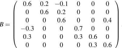
B=
0.6 0.2 −0.1 0 0 0
0 0.6 0.2 0 0 0
0 0 0.6 0 0 0.4
−0.3 0 0 0.7 0 0
0.3 0 0 0.3 0.6 0
0 0 0 0 0.3 0.6
, (2)
Figure 1a shows its topology (self-connections are removed). The nodes evolve and interact with each other through the Granger causal connections, resulting in the random processes plotted in Figure 1b. Therefore, matrixBnot only illustrates the dynamic rules that govern the evolution of the system, but also captures a linearcausality networkthat describes the (Granger) casual relations between nodes.
2.1 Sparse Network Learning by Penalized Maximum Likelihood Estimation
Givennobservations of the dynamical networkx1,···,xn, we wish to estimateB. Due to Markov-chain property, we can write the likelihood ofBas
L(B|x1,···,xn) = n
∏
t=2
f(xt|xt−1,···,x1,B)f(x1|B) =
n
∏
t=2
f(xt|xt−1,B)f(x1|B).
The exact maximum likelihood (ML) estimate requires solving a nonlinear optimization problem. For simplicity, researchers often use theconditionallikelihood where the initial statex1is assumed
to be fixed. Due to normality, we have the conditional likelihood
Lc(B) = n
∏
t=2
f(xt|xt−1,B) = n
∏
t=2
(2π)−p/2|Σε|−1/2exp{−1
2(xt−Bxt−1) TΣ−1
ε (xt−Bxt−1)}.
So the (conditional) ML estimate ofBcan be obtained by solving
min B 1 2 n
∑
t=2LettingY = [xT2,xT3,···,xTn]T,X = [xT
1,xT2,···,xnT−1]TandA=BT, we can formulate the problem
in matrix form:
AML=arg min A l(A) =
1
2kY−X Ak
2
F.
For convenience, we use Ainstead of B to represent the network in the remainder of the paper. Note thatai j describes the directed connection strength from nodeito node j. The estimate ˆAML has been investigated and applied to many real-world data. For stationary process, the consistency and asymptotic efficiency of ˆAML are analyzed in Reinsel (1997). The small-sample properties are discussed in L¨utkepohl (2007).
Nevertheless, the plain ML estimation is not ideal for network learning. In practice, X usually demonstrates high collinearity, especially when some nodes have similar dynamical behaviors and when the number of observations is limited. Moreover, the ML estimation does not promote sparsity and consequently the resulting model is difficult to interpret. To improve prediction accuracy and obtain interpretable model,shrinkage estimationis necessary. It can be done by adding a penalty and/or constraint. For example, we can estimateAvia penalized maximum likelihood (PML):
ˆ
APML=arg min
A l(A) +P(A;λ). (3)
We consider only the additive penalties and denoteP(A;λ) =∑i,jP(ai j;λi j), whereP(·)is a penalty function applied to each component ofA, andλi j is the corresponding regularization parameter(s). Alternatively, constraints can also be used. See Section 2.3 and Section 3.4.
Different penalties have been proposed. The famous Lasso (Tibshirani, 1996) solves the ℓ1
penalized problem. It is fast in computation. Nevertheless, Lasso suffers from some drawbacks such as selection inconsistency, estimation bias and incapability of dealing with collinearity, in particular. Zou and Hastie (2005) propose the elastic net (eNet for short in this paper) which adds an additional ridge regularization (Hoerl and Kennard, 1970) to deal with collinearity and large noise. However, the design counteracts sparsity to some extend and may bring the double shrinkage issue. Some nonconvex alternatives, including the ‘ℓ0+ℓ1’ SCAD (Fan and Li, 2001) and the
‘ℓ0+ℓ2’ hard-ridge (She, 2009, 2012), are advocated to promote more sparsity. However, due to nonconvexity, the convergent solution may be only locally optimal and depend on the choices of the initial point. They are also more computationally expensive than convex approaches. Therefore, we do not consider nonconvex regularizations hereinafter.
2.2 The S2Network Learning
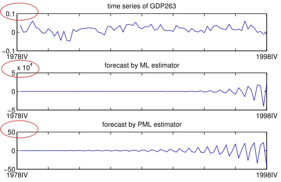
Many real-world time series (possibly after proper transformations such as taking logarithm and/or differencing) are stationary. Stationary and nonstationary processes behave in fundamentally dif-ferent manners. See Figure 2. For a stationary process, its probability distribution is invariant with respect to the shift in time. In the nonstationary process, however, we can clearly see drift-ing and trenddrift-ing behaviors. In practice, given raw observations sampled from a dynamical system, researchers first stationarize the time series and then input them to the ML/PML estimator. The resulting estimate ˆAML/AˆPMLis used for analysis and forecast. Unfortunately, however, the station-arity requirement may be violated by ˆAML/AˆPML in practice. Figure 3 shows a real-data example. We apply ML and PML (adopting the ℓ1 penalty) respectively to the U.S. macroeconomic data
0 50 100 150 −20
−10 0 10 20
stationary process
X
0 50 100 150
−1 −0.5 0 0.5
1x 10
26 non−stationary process
t
X
Figure 2: Example of stationary and nonstationary processes. The number of nodes isp=50. The stationary process hasρ(A) =0.95 and the nonstationary process hasρ(A) =1.05.
1978IV 1998IV
−0.1 0 0.1
time series of GDP263
1978IV−5 1998IV
0 5x 10
4 forecast by ML estimator
1978IV 1998IV
−50 0 50
forecast by PML estimator
Figure 3: Forecasts of GDP263 given by ML and PML estimation. The time series of GDP263 is obtained from seasonal observations between 1978:IV and 1998:IV. It is a stationary process. However, the forecasts given by ML and PML exhibit nonstationary behaviors. ρ(AˆML) =1.171,ρ(AˆPML) =1.073.
In this paper, we propose the framework ofstationary-sparse(S2) network learning to address
the limitation of PML to guarantee the stationarity property of the network. We invoke the station-arity condition and design an efficient algorithm to solve the optimization problem.
A random process as in (1) is stationary if and only if its spectral radius ρ(A) satisfies the stationarity condition:
ρ(A)=∆ max
i |λi|<1, (4)
whereλiis theith eigenvalue ofA, possibly complex, and| · |is the complex norm (Reinsel, 1997). This leads to the following optimization problem:
min
A f(A) = 1
2kY−X Ak
2
F+P(A;λ)
s.t.ρ(A)<1.
(5)
Nevertheless, problem (5) is extremely challenging due to the fact thatρ(A)is a nonconvex and non-Lipschitz-continuous function ofA. An optimization method proposed by Curtis and Overton (2012), which combines sequential quadratic programming and gradient sampling, sheds some light on solving (5). However, at each iteration, the gradient sampling needs to sample p2 points and calculate the gradient of the spectral radius at each point. As discussed in Overton and Womersley (1988), calculating the gradient of spectral radius for a single point is already a challenging and computationally demanding problem. It is prohibitive to do so forp2points at each iteration in our problem. Moreover, this method only guaranteesρ(A)≤1, notρ(A)<1.
We consider a reasonable convex relaxation of (4) as the stationarity constraint:
kAk2
∆
=max
i |νi| ≤1,
whereνi is theith singular value ofAand thuskAk2is the spectral norm. For an arbitrary square
matrix, we haveρ(A)≤ kAk2, where the equality holds whenAis a symmetric matrix. In all our
applications, we haveρ(A)<1.
TheS2learning problem is given by ˆ
AS2 =arg min
A f(A)
s.t.kAk2≤1.
(6)
Note that the stationarity constraint also has a “shrinking” effect on the estimate, which contributes to the shrinkage estimation we are seeking, as discussed in Section 2.1.
2.3 The “Berhu” Penalty for Sparsity Pursuit and Model Decorrelation
linear at large ones, which makes it more robust to outliers than the squared-error criterion. Inspired by the Huber function, Owen (2007) designed a convex penalty function Berhu
PB(t;λ,M) = (
λ|t| if|t| ≤M λt2+M2
2M if|t|>M.
(7)
As implied by its name, Berhu reverses the composition of Huber: it is linear at small values and quadratic at large ones.
−2 0 2
0 0.5 1
Lasso penalty
−2 0 2
0 0.5 1 1.5 2 ridge penalty
−20 0 2
1 2 3 4
eNet penalty
−2 0 2
0 0.5 1 1.5
Berhu penalty
−2 0 2
−2 −1 0 1 2 Soft thresholding
−2 0 2
−2 −1 0 1 2 ridge thresholding
−2 0 2
−2 −1 0 1 2 eNet thresholding
−2 0 2
−2 −1 0 1 2 Berhu thresholding
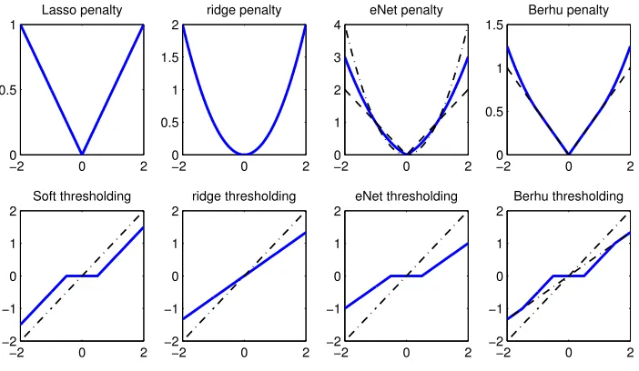
Figure 4: Penalty functions and corresponding solutions.
Figure 4 compares Berhu with the ridge penalty PR(t;η) = 12ηt2, Lasso PL(t;λ) =λ|t| and eNetPE(t;λ,η) =λ|t|+12ηt2. The upper panel plots the functions, while the lower panel shows their corresponding solutions in the univariate and orthogonal case (see Section 3.2 for details). The ridge penalty shrinks the coefficients to compensate for collinearity. But it can not produce exact zero coefficients in the estimate. The Lasso soft-thresholds the coefficients to encourage sparsity. However, it does not shrink the large coefficients effectively and does not work well for correlated data. The eNet incorporates the ridge component into the ℓ1. However, the singularity of the penalty function at zero is smoothed out to some extent by the ℓ2 part, which may lead to
an estimate not parsimonious enough. Also, it tends to over-shrink medium and large coefficients (Zou and Hastie, 2005). Berhu overcomes these drawbacks by using a nonlinear fusion of theℓ1
andℓ2 penalties: for small coefficients, theℓ1 regularization is enforced to achieve sparsity; for
large coefficients, theℓ2regularization is enforced to compensate collinearity (Hoerl and Kennard,
and shrinks large ones. It does selection and decorrelation separately, which better serves two important objectives of network learning: accurate prediction and parsimonious representation.
SubstitutingPB(A;λ,M)into (6), we focus on solving
arg min
A fB(A) = 1
2kY−X Ak
2
F+PB(A;λ,M)
s.t.kAk2≤1.
(8)
In this problem,PB(A;λ,M)is typically nondifferentiable at zero and piecewise. The stationarity constraint adds more difficulties to the problem. Moreover, in practice we are frequently confronted with large-scale networks. Hence, an efficient and scalable algorithm is desired for S2 network learning.
3. Computation of BISPS
In this section, we propose an algorithm namedBerhu iterative sparsity pursuit with stationarity (BISPS) to effectively solve theS2 learning problem (8). Some algorithms based on conventional techniques will be developed first. They suffer from high computational complexity, poor numerical accuracy, and/or insufficient sparsity. We then propose the novel BISPS which is easy to implement and computationally efficient. Finally, to facilitate BISPS for ultra-high dimensional problems, we propose the quantile thresholding iterative screening (QTIS). Convergence proofs are provided. We assume the data matrices X,Y has been centered before all the computation. Precalculations ΣX X=∆ XTX andΣXY =∆ XTY help avoid repeated computation.
3.1 Algorithms Based on Conventional Techniques
Problem (8) can be reformulated and then solved by well-known optimization techniques, such as semidefinite programming, projected subgradient method, and alternating direction method of multipliers. We briefly discuss these algorithms before introducing BISPS.
3.1.1 SEMIDEFINITEPROGRAMMING
Problem (8) can be reformulated as a semidefinite programming (SDP) problem
min A fB(A)
s.t.
I A
AT I
0
and can be solved by general SDP solvers. However, since most of the SDP solvers use interior point methods, they suffer from extremely high space complexity. For example, we tried the popular SDP solvers SeDuMi (Sturm, 1998) and SDPT3 (T¨ut¨unc¨u et al., 2003) using MATLAB7.11.0 on a PC with 4GB memory; when the number of network nodes is larger than 100, both solvers ran out of memory.
3.1.2 PROJECTEDSUBGRADIENTMETHOD
Define the subgradient of fB(A)atAas
where∂PB(A;λ,M)is the subdifferential (Alber et al., 1998) ofPB(·), and∇l(A)is the gradient of l(A):∇l(A) =ΣX XA−ΣXY. The projected subgradient method (PSGM) for problem (8) computes a sequence of feasible points{Ak}with the update rule
Ak+1=Π(Ak−αkUk; 1),whereUk∈∂fB(Ak),
until Ak satisfies 0∈∂fB(Ak). The operator Π stands for spectral norm projection defined in Lemma 5.
PSGM is simple to implement. At each step, one performs subgradient evaluation and spectral norm projection. Nevertheless, due to the uncertainty of the subgradient at the non-differentiable point of the penalty function, it suffers from slow convergence and insufficiency of sparsity. For example, in an experiment where the number of nodesp=100 and number of observationsn=80, it does not converge yet after 104iterations.
3.1.3 ALTERNATINGDIRECTIONMETHOD OFMULTIPLIERS
The basic idea of alternating direction method of multipliers (ADMM) is to split the objective function and variables and update them in an alternating fashion (Boyd et al., 2010). To apply ADMM for solving problem (8), we reformulate it as
min A,B,C
1
2kY−X Ak
2
F+PB(B;λ,M)
s.t.
A A
=
B C
,
andkCk2≤1.
The augmented Lagrangian can then be written as Lρ1,ρ2(A,B,C,Γ1,Γ2) =
1
2kY −X Ak 2
F+
PB(B;λ,M) +tr{ΓT1(A−B)}+tr{ΓT2(A−C)}+
ρ1
2kA−Bk2F+ ρ2
2kA−Ck2F, whereΓ1 andΓ2 are
Lagrangian multipliers andρ1 andρ2 are the augmented Lagrangian parameters. The iteration of
ADMM consists of the following steps
Ak+1= (ΣX X+ρ1I+ρ2I)−1(ΣXY−Γk1−Γk2+ρ1Bk+ρ2Ck),
Bk+1=ΘB(Ak+1+Γk1/ρ1;λ/ρ1,M),
Ck+1=Π(Ak+1+Γk2/ρ2; 1),
Γk1+1=Γk1+ρ1(Ak+1−Bk+1),
Γk2+1=Γk2+ρ2(Ak+1−Ck+1),
whereΘB is the thresholding operator of Berhu—see Appendix A for detail. Note that matrix in-version is involved in updatingA, which increases computational difficulty. The penalty parameters ρ1 andρ2 have to be large enough; the choices of them have been shown to influence the number
of iterations significantly. To speed up convergence in practice, one can replace the constantsρ1
andρ2with two sequences{ρk1}and{ρk2}respectively, whereρk1andρk2vary along the iterations
In summary, although we have implemented some algorithms based on conventional techniques for the S2 network learning problem, they are unable to cope with large-scale networks. A more efficient and scalable algorithm is in great need.
3.2 The Berhu Thresholding Operator
Section 2.3 advocates the Berhu penalty forS2 network learning. However, in the original paper (Owen, 2007), Berhu was solved through cvx (Grant and Boyd, 2008). Practical applications call for the development of much faster algorithms. In this paper, we reparameterize Berhu and develop its coupledthresholding rule, which allows us to solve the Berhu sparsity pursuit—problem (3) with Berhu penalty—in a simple and efficient way. This formulation facilitates easy parameter tuning. Also, it helps us understand the essence of Berhu.
Letη=λ/M. Reformulate the Berhu penalty (7) as
PB(t;λ,η) = (
λ|t| if|t| ≤λ/η
η2t2+λ2
2η if|t|>λ/η.
(9)
Define a thresholding rule
ΘB(t;λ,η) =
0 if|t|<λ
t−λsgn(t) ifλ≤ |t| ≤λ+λ/η
t
1+η if|t|>λ+λ/η.
(10)
It can be verified that, as shown in Lemma 3,ΘB(·;λ,η)is the coupled thresholding rule for the Berhu penaltyPB(·;λ,η):
PB(t;λ,η) =
Z |t|
0 (sup{s:
ΘB(s;λ,η)≤u} −u)du.
For the multivariate case, the Berhu thresholding operator is applied elementwise.
With ΘB(·;λ,η), we can solve the Berhu sparsity pursuit (without the stationarity constraint) using a simple iterative procedure:
Ak+1=ΘB(Ak+αk(ΣXY−ΣX XAk);λ,η). (11)
SincePB(·;λ,η)is convex, algorithm convergence is guaranteed givenαk≤
√
2/kXk2(She, 2012).
It is worth pointing out that, based on the construction rule (13), we can also define the thresh-olding operators for other penalties including Lasso, eNet and the ridge penalty, as shown in Fig-ure 4. The Berhu thresholding operatorΘB(t;λ,η)offers a nonlinear fusion of the soft thresholding operator (coupled with Lasso) ΘS(t;λ) =sgn(t)(|t| −λ)1|t|≥λ and the ridge thresholding opera-torΘR(t;η) = 1+tη. For the difference between the Berhu thresholding and the eNet thresholding
ΘE(t;λ,η) =1+1ηsgn(t)(|t| −λ)1|t|≥λ, see the discussion in Section 2.3. 3.3 The BISPS Algorithm
Algorithm 1The Berhu iterative sparsity pursuit with stationarity (BISPS)
Input: data matrixΣX X,ΣXY; regularization parametersλ,η; stopping criteriaδ1,δ2,M1,M2; initial
estimateA0.
{Letk · k2denotes the spectral norm andk · kmaxdenote the elementwise max-norm.}
k0←any constant satisfyingk0>kXk2;
k←0;
repeat
1) B0←Ak+ 1
k2 0
(ΣXY−ΣX XAk);
2) j←0;P0←0;Q0←0;
repeat
2.1) Cj=ΘB(Bj+Pj;λ/k02,η/k20);
2.2) Pj+1=Bj+Pj−Cj; 2.3) Bj+1=Π(Cj+Qj; 1); 2.4) Qj+1=Cj+Qj−Bj+1;
j← j+1;
untilkBj−Bj−1kmax≤δ2or j≥M2
3) Ak+1←Bj; k←k+1;
untilkAk−Ak−1kmax≤δ1ork≥M1
ˆ A←Ak;
Output: Aˆ.
Π. Parameter k0 can be set to any constant that is larger than the spectral norm of X. No ad
hocalgorithmic parameters, such asρ1,ρ2 in ADMM and αk in PSGM, are involved. The inner iteration of Step 2 often converges within 10 steps in practice, where matricesC,P,Qare auxiliary variables that contribute to fast convergence of the procedure. Step 2.1 is to enforce sparsity by Berhu thresholding and Step 2.3 is to project the estimate to the convex set{B:kBk2≤1}. The
outer iteration has only a simple update step and converges fast. As a result, the algorithm is computationally efficient as well as easy to implement.
The convergence of BISPS is theoretically guaranteed. For simplicity, we assume the inner iteration is run till convergence. Theorem 1 states that Algorithm 1 solves theS2network learning problem.
Theorem 1 Supposeλ≥0,η≥0 andλη=6 0. Given k0 >kXk2, for any initial value A0, the
sequence of iterates {Ak} produced by Algorithm 1 converges to a globally optimal solution to problem(8).
See Appendix A for the detailed proof.
BISPS has more flexibility and generality. Though it is designed with the Berhu penalty, by replacingΘB with an appropriate thresholding operator in Step 2.1, the algorithm allows for any convex penalty forS2learning. Moreover, if Step 2.2 to Step 2.4 are removed, Algorithm 1 reduces to the Berhu sparsity pursuit (11).
stationarity condition (4), we accept and output this solution. Otherwise, we rerun Algorithm 1 with Step 2.2 to Step 2.4 included. 2) Moreover, we can take advantage of the fact thatAk+1is sparse and the number of singular values ofAk+1that are larger than 1 is much smaller than p. The singular value thresholding algorithm (Cai et al., 2010), among some other fast algorithms, calculates only the singular values that are above a threshold and their corresponding singular vectors, which is computationally efficient for large sparse matrix and thus fits our problem well. We use the package MODIFIED-PROPACK provided by Lin (2011) to calculate the partial SVD with threshold being 1. For p=500,n=100, the partial SVD, compared with the original SVD, can accelerate the calculation by up to 30 times.
3.4 Quantile Thresholding Iterative Screening
Nowadays, a great challenge for network identification and statistical learning comes from the large scale of the system. For example, for a network withp=1000 nodes, the number of variables in the transition matrix is as large asp2=106, which poses a great challenge for any estimation algorithm in scalability and stability. As a result, ultra-high dimensional learning has become a hot topic (Fan et al., 2009; Fan and Lv, 2010) . For regression problems, under the assumption that the number of nonzero coefficients is far smaller thann, screeningtechniques can be used to coarsely select the variables before finer estimation. This idea can be adopted in network identification: if one is sure that the average number of connections for each node is much less than ⌈µn⌉ (say µ=0.8) or the total number of connections in the network is much less than ⌈µpn⌉, one can first use fast screening techniques to selectm=⌈µpn⌉candidate connections, and then apply BISPS restricted on the candidate connections for further selection and estimation. If the screening technique can include all the true connections with high probability, dramatic computational gain can be attained with mild performance sacrifice.
Independence screening methods, such as the sure independence screening (SIS) (Fan and Lv, 2008) can be applied to preselect variables in a supervised manner. Applied to network learning, SIS sorts the elements ofW=XTY by magnitude in a decreasing order and defines a reduced model
M
µ={(i,j):|wi j|is among themlargest of all,1≤i,j≤p}.This method is simple and fast, but it relies on the assumption that the predictors areindependent, since it only studies the marginal correlation betweenY andXand selects the variables accordingly. In network settings, the nodes are interacting dynamically with each other, so there is usually high collinearity in the data. In such cases, SIS is too greedy and misses many true connections.
To derive a new screening technique that can handle network data, we first observe that SIS corresponds to the first step of the iterative procedure in (11) with A0=0 and hard thresholding ΘH(t;λ) =t1|t|≥λ with a properly chosenλ. This inspires us to apply an iterative procedure for screening: starting fromA0=0, repeat
1) Ak+1←Ak−k12 0
(ΣX XAk−ΣXY);
2) λk+1←(m+1)th largest element ofAk+1in magnitude;
3) Ak+1←ΘH(Ak+1;λk+1); 4)
M
k+1µ ← {(i,j):|aki j+1| 6=0,1≤i,j≤p};
until
M
kWe call this screening procedure thequantile thresholding iterative screening(QTIS). As shown in Step 2 and Step 3, QTIS does not select variables using a fixed thresholding parameterλ. Instead, it uses adynamicthreshold to keep a fixed numbermof nonzero elements at each iteration. The quantile parameter µ determines the number of variables to be selected. In comparison to SIS which ranks the connections based onXTY, the iterative nature of QTIS lessens the greediness by repeatedly updating the importance of each candidate connection with a theoretical guarantee of convergence.
Theorem 2 Given k0>kXk2, for any0<µ≤1, the sequence of iterates{Ak}generated by QTIS
has the function value decreasing property that l(Ak+1)≤l(Ak),where l(A) = 1
2kY−X Ak 2
F, and Ak
satisfieskAkk0≤m, wherek · k0denotes the number of nonzero elements.
See Appendix B for the detailed proof.
In practice,
M
µ usually stops changing after less than a hundred iterations. The number of unknowns is reduced from p2to⌈µpn⌉effectively by a small amount of computation. Then, more involved and sophisticated estimation, for example, BISPS, can be performed to the reduced model. It is much faster than applying BISPS directly ifp2≫n. In addition, QTIS provides BISPS with a sparse pattern, which facilitates the fast computation of partial SVD.To apply BISPS on
M
µ, we use element-wise penalty parametersλi j’s and setλi j=∞if(i,j)∈/
M
µ.This simple modification guarantees that only elements in
M
µwill be selected by BISPS.3.5 Two-dimensional Selective Cross Validation for Tuning
The reparameterization of Berhu (9) separates the roles ofℓ1andℓ2regularizations; each of them
is associated with a regularization parameter, namelyλforℓ1andηforℓ2. This provides important guidelines for parameter tuning. Based on our experience, the estimate is not very sensitive toη, so a full two-dimensional grid search is not necessary. Instead, we search along several one-dimensional solution paths including oneη-path and threeλ-paths:
• Step 1 : Run theη-path (λ=0). Do ridge regression with a grid of values forη, and choose the optimalη∗using AIC (Akaike, 1974).
• Step 2 : Run 3λ-paths with η=0.5η∗,0.05η∗,0.005η∗ respectively. For each value of η,
run BISPS with a grid of values forλ, and find the optimal oneλousing theK-fold selective cross-validation (SCV) (She, 2012). This results in threeλo’s, one from each path. Choose the optimal one from them and let it be the optimal thresholding parameterλ∗. The pair (λ∗,
η∗) is our final choice of the two parameters.
4. Stationary Bootstrap (SB) Enhanced Network Learning
TheS2learning framework proposed in Section 3 is an effective technique to identify stationary and sparse network. Nevertheless, a “one-time” estimate, without any p-value or confidence interval, provides only limited guidance in identifying the true network topology. In fact, whatever inference method is used, there will be uncertainty underlying the variable selection procedure. It would be greatly helpful if one could provide some kind of uncertainty measure for such an estimate. In our case, we would like to find a certain confidence measure for the estimated topology. This can be done by assigning a probability for the existence of each connection. Hence, we use bootstrap (Efron, 1979). In this section, we propose thestationary bootstrapenhanced BISPS (SB-BISPS) which provides a confidence level about whether a connection exists in the network by measuring the frequency with which it is chosen by the BISPS algorithm.
4.1 The SB-BISPS Framework
The SB-BISPS procedure completes the BISPS (or QTIS+BISPS) algorithm with a stationary boot-strap resampling step. The SB-BISPS is described as follows.
• Step 1 : Run BISPS over the original data set
X
. Record the pattern of ˆA, which is ap×p binary matrixΦ= [φi j]1≤i,j≤pdefined as:φi j= (
1 if ˆai j 6=0
0 if ˆai j =0.
• Step 2 : DrawBstationarybootstrap samples from
X
. Repeat Step 1 for each sample. Record Φ∗j for the jth sample.• Step 3 : Compute the matrix F = [fi j]1≤i,j≤p ofconnection occurring frequency(COF) by adding up all the patternsΦ∗j’s and normalizing the result byB:
F= 1
B
B
∑
j=1
Φ∗j.
Given a sufficiently largeB, fi j is a good approximation of the probability for BISPS to select connectionai j, which serves as a measure of how confident we are with the existence of this con-nection. For example, if fi j =80%, it means that in 80% of the bootstrap samples, a connection from nodeito node jis detected. So we can say the probability for the existence of this connection is (approximately) 80%. We can use a cutoff value f∗to threshold the COF matrix, and choose only the connections with fi j≥ f∗for further analysis. This renders us a sparse topology that shows the most significant connections within the network.
4.2 Stationary Bootstrap
dependency structure in bootstrapping. Techniques such as resampling blocks of consecutive ob-servations or resampling “blocks of blocks” can be used (Kunsch, 1989). The basic idea is that, despite the dependence of individual observations, blocks of observations can be approximately independent with each other given a proper block sizel.
When a time series is stationary, it is natural to maintain this property in the bootstrap samples. The stationary bootstrap (Politis and Romano, 1994) is a method with this property. It is based on resampling blocks of random lengths, where the length of each block follows a geometric distri-bution with mean 1/γ. We apply a simple approach to conduct such resampling. Given thatx∗i is chosen to be theJth observationxJin the original time series, we choosex∗i+1based on the following
rule:
x∗i+1=
(
xJ+1with probability 1−γ
picked randomly fromx1,···,xnwith probabilityγ.
Similar with block bootstrap, where the block sizelhas to be determined, the value ofγshould be chosen properly. Fortunately, the sensitivity ofγin stationary bootstrap is less than that oflin block bootstrap.
5. Experiments
In this section, we present the experimental results on synthetic data and demonstrate the effective-ness of the proposedS2network learning framework.
5.1 Performance Measures and Experiment Settings
To examine the performance of the proposed methods, we define the following measures.
• Stationarity violation percentage (Pv): InNrepeated experiments, if there areNvexperiments in which the estimate ˆAviolates the stationarity condition (4), then the stationarity violation percentage is defined asPv=Nv/N.
• Miss rate (Pm): Ifai j 6=0,aˆi j=0, we say there is a miss. DenoteCmas the total number of misses andCnzas the number of nonzero entries inA. The miss rate is defined asPm=Cm/Cnz.
• False alarm rate (Pf): Ifai j=0,aˆi j 6=0, we say there is a false alarm. DenoteCf as the total number of false alarms andCz as the number of zero entries in A. The false alarm rate is defined asPf =Cf/Cz.
• Testing error (T E): The testing error is defined asT E= 1
ntkY
t−XtAˆk2
F, whereYt andXt are testing data, andnt is their length. For time series, the testing data are collected right after the training data.
• Computation time: The averaged running time of an algorithm. All the algorithms are run in MATLAB7.11.0 on a PC with 4GB memory.
we use this estimate to forecast xt+h, denoting the forecast as ˆxt+h and the forecasting error as
eht =kxt+h−xˆt+hk22. This process is repeated fort=W,···,W+N−1 as we shift the window.
N is the number of window shifting that satisfies 1≤N≤T−W−h−1. Then the rolling MSE for horizonhis defined asMSErollingh = 1
N∑ W+N−1
t=W eht. When using ˆAt to forecastxt+h, we should do pseudo out-of-sample forecasting. That is, we assume the observations aftertare not available and consequently we need do h-step-ahead forecast. For our model (1), this should be done as:
ˆ xt+h=Aˆ
T
t xˆt+h−1forh≥1, where ˆxt ∆
=xt whenh=1. The testing error defined above corresponds to the rolling MSE forh=1.
We generate the p×ptransition matrixAwith both sparsity and stationarity properties. First, the topology is generated from a directed random graphG(p,ξ), where the edge from one node to another node occurs independently with probabilityξ. Then the strength of the edges is generated independently from a Gaussian distribution. This process is repeated until we obtain a matrixAthat has a desired spectral radius 0.9<ρ(A)<1. We setξ=10/p,Σε=σ2I,σ2=10.
The regularization parameters are chosen by SCV as described in Section 3.5. For aλ-path, we use a grid of 100 values forλ, which is picked from the interval[0,kA0+XTY−XTX A0kmax]. The
initial estimate is simply set asA0=0. For anη-path, we use a grid of 76 values forη, which is picked from the interval[2−10,25]. The number of folds for SCV is set to beK=5. All the statistics
collected are averaged overN=100 times of window shifting. The length of testing datant=200.
5.2 Performance of BISPS
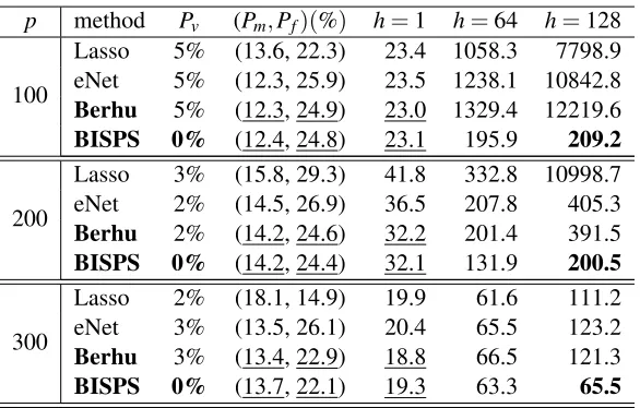
We compare the performance of BISPS with Lasso, eNet and Berhu—we use the penalty name to denote the corresponding PML estimation. The number of observations isn=80. Table 1 shows the experiment results for different network sizes, namelyp=100,200,300. Recall that for a network with sizep, the number of unknown parameters isp2. For example, for the network with 300 nodes, the number of parameters to be estimated is 9×10⁴, which is extremely high compared with the number of observations 80.
Among the three penalties, the Lasso solution gives higher miss rates. This is because when some predictors are correlated, Lasso tends to choose only a part, or even none, of them. As a result, Lasso sometimes “over-shrinks” the estimate. The eNet and Berhu, in such cases, tend to include all the correlated predictors, thanks to the ℓ2 part in the penalties. However, the sparsity of the eNet solution is affected by theℓ2regularization, so it gives high false alarm rates. On the other hand, Berhu has improved eNet to some extend by enforcing the ℓ2 regularization only to
large coefficients. As a result, Berhu achieves the smallest testing errors (h=1) among the three penalties.
As shown byPv, no matter what penalty is used, it is possible for PML to give a nonstationary estimate, whereas the proposedS2learning and BISPS can guarantee the stationarity property of ˆA.
This indicates that adding the stationarity constraint into the sparsity pursuit does effectively prevent the estimate from becoming nonstationary. Meanwhile, theS2estimate can achieve a comparable estimation and detection accuracy with the PML estimate. Table 1 gives the rolling MSEs for different horizonsh to illustrate both the short term and long term forecasting performance. For PML estimates, the rolling MSEs grow explosively with h due to the existence of nonstationary estimates, while those of BISPS accumulate much more slowly.
p method Pv (Pm,Pf)(%) h=1 h=64 h=128
100
Lasso 5% (13.6, 22.3) 23.4 1058.3 7798.9
eNet 5% (12.3, 25.9) 23.5 1238.1 10842.8
Berhu 5% (12.3, 24.9) 23.0 1329.4 12219.6
BISPS 0% (12.4, 24.8) 23.1 195.9 209.2
200
Lasso 3% (15.8, 29.3) 41.8 332.8 10998.7
eNet 2% (14.5, 26.9) 36.5 207.8 405.3
Berhu 2% (14.2, 24.6) 32.2 201.4 391.5
BISPS 0% (14.2, 24.4) 32.1 131.9 200.5
300
Lasso 2% (18.1, 14.9) 19.9 61.6 111.2
eNet 3% (13.5, 26.1) 20.4 65.5 123.2
Berhu 3% (13.4, 22.9) 18.8 66.5 121.3
BISPS 0% (13.7, 22.1) 19.3 63.3 65.5
Table 1: Performance comparison of BISPS with Lasso, eNet and Berhu.n=80.
forh=1,···,100 using ˆALassoand ˆABISPS respectively and compare them withxt+hobserved from the true model. The results are plotted in Figure 5. We can easily see that ˆx(AˆBISPS)gives a reason-able imitation of the true system. The nonstationary estimate ˆx(AˆLasso), however,blows upquickly and behaves completely differently from the true model. This indicates that ensuring a stationary estimate is indeed crucial.
5.3 Performance of QTIS
To examine the performance of QTIS for connection screening, we first compare it with the sure independence screening (SIS) (Fan and Lv, 2008) by examining their ability to include all the true connections, which can be measured by the miss rate. Simulation is done for networks with dif-ferent sizes, namely p=300,400,500. The sample sizen=80. Independence screening methods, including SIS, are very popular in ultra-high dimensional problems for dimension reduction and variable selection. However, our finding is that such methods can perform very poorly for network learning. As shown in Figure 6, it is possible for SIS to miss even more than half of the true connec-tions. One possible reason is that, because of the evolving processes, correlation exits ubiquitously in dynamical networks. As a result, independence screening is not appropriate for network learning. On the other hand, the proposed QTIS algorithm considers the correlation issue and thus can obtain much smaller miss rates than SIS. Also, its performance is more robust to the choice of the quantile parameterµ.
0 10 20 30 40 50 60 70 80 90 100 −20
0 20
h
0 10 20 30 40 50 60 70 80 90 100 −1
0 1x 10
20
h
0 10 20 30 40 50 60 70 80 90 100 −20
0 20
h
Figure 5: Comparison of BISPS and Lasso in terms of forecasting performance. Top: sample from the true model; Middle: forecast from the nonstationary estimate ˆALasso; Bottom: forecast from the stationary estimate ˆABISPS.
0.6 0.7 0.8 0.9 1 0.2
0.25 0.3 0.35 0.4 0.45 0.5 0.55
quantile paramter
miss rate
p=500, QTIS p=500, SIS p=400, QTIS p=400, SIS p=300, QTIS p=300, SIS
Figure 6: Miss rate comparison for QTIS and SIS.n=80.
6. Application to U.S. Macroeconomic Data
3000 400 500 600 700 800 50
100 150 200 250
p
computation time
QTIS+BISPS BISPS
(a) computation time
3000 400 500 600 700 800
0.1 0.2 0.3 0.4 0.5
p
miss rate
QTIS+BISPS BISPS
(b) miss rate
300 400 500 600 700 800 0.2
0.25 0.3 0.35 0.4
p
testing error
QTIS+BISPS BISPS
(c) testing error
Figure 7: Performance of QTIS+BISPS, compared with applying BISPS to a full model. n=80.
Category Lasso BISPS Category Lasso BISPS
1. GDP 0.589 0.445 7. Prices 1.971 1.874
2. IP 0.846 0.576 8. Wages 0.552 0.207
3. Employment 0.936 0.711 9. Interest rate 1.443 0.738
4. Unempl. rate 0.289 0.165 10. Money 0.114 0.065
5. Housing 0.071 0.033 11. Exchange rates 0.370 0.107
6. Inventories 0.506 0.217 12. Stock prices 0.254 0.100
Table 2: Normalized Rolling MSE of Lasso and BISPS for each category.
h 1 2 4 8 16 32
Lasso 0.017 0.021 0.029 0.365 329.9 3.1×10⁸
BISPS 0.017 0.018 0.019 0.020 0.020 0.018
Table 3: Rolling MSE of Lasso and BISPS for different horizons.
6.1 Comparison of Rolling MSE
We first study the data set by category, considering that multiple time series explain the interactions of the indices in each category. To each of the 12 categories, we apply Lasso and BISPS respectively with the horizonh=1 and the rolling window sizeW =0.8×p, where pis the number of time series (network size). Table 2 shows the rolling MSEs of the Lasso and BISPS, normalized by that of the AR(4) model, which is a conventional benchmark of macroeconomic forecasting.
Compared with the AR(4) model, both Lasso and BISPS, based on a VAR model, have attained much smaller forecasting errors, except for Category 7 (prices). Therefore, by introducing the Granger causal interactions between different indices, we can build a multivariate network model that is more accurate than the univariate AR model in capturing the evolution of the U.S. macroe-conomics, given the same amount of observations. The exception of Category 7 may be due to the higher lag order used in the univariate AR model.
Moreover, we note that BISPS gives smaller forecasting errors than Lasso for all the 12 cate-gories of macroeconomic time series. It indicates that adopting a fusion ofℓ1andℓ2 penalties and
imposing the stationarity constraint can capture the network dynamics more accurately and achieve a stronger capability of forecasting. To further support this conclusion, we apply Lasso and BISPS respectively to all the 108 variables withW=0.8×pand different horizonsh. The rolling MSEs forh=1,2,4,8,16,32 is recorded in Table 3. As the horizon increases, the rolling MSE of Lasso grows exponentially, which clearly indicates that some estimates of the Lasso are nonstationary and thus fail to forecast for large horizons. On the other hand, the rolling MSE of BISPS stays stable for different horizons. This phenomenon is similar to what is shown in Figure 5. They have illustrated the fundamental difference of theS2learning from the plain PML estimation.
6.2 Bootstrap Analysis
In this experiment, we apply the SB-BISPS to the macroeconomic data before and after the “Great Moderation” (Davis and Kahn, 2008) and analyze the changes in their Granger causal connections. As the economic structure of U.S. has gone through huge changes in the Great Moderation in mid-1980, we expect to see significantly different causality networks before and after mid-1980. Hence, we divide the time series into two periods, the pre-Great Moderation period and the post-Great Moderation period, and apply SB-BISPS separately to the two periods.
For the pre-Great Moderation period, we use the data from 1960:I to 1979:IV as training set (80 observations); for the post-Great Moderation period, we use the data from 1985:I to 2004:IV (80 observations). The stationary bootstrap samples are obtained using the R functiontsboot (Dalgaard, 2008) with default parameter values. The number of stationary bootstrap samples is set to beB=
0 0.1 0.2 0.3 0.4 0.5 0.6 0.7 0.8 0.9 1
(a) pre-Great Moderation
0 0.1 0.2 0.3 0.4 0.5 0.6 0.7 0.8 0.9 1
(b) post-Great Moderation
Figure 8: COFs of the pre-Great Moderation period and the post-Great Moderation period.
GDP251 GDP253 GDP254 GDP255 GDP256 GDP257 GDP258 GDP259 GDP260 GDP261 GDP263 GDP264 GDP265 GDP266 GDP269 GDP270 GDP271 GDP275 GDP277 GDP278 GDP281 GDP282 GDP285 LBMNU GDP274_2 GDP275A GDP275_1 GDP275_3 GDP276_6 GDP276_7 GDP277A GDP278A GDP285A GDP285_1 GDP285_2
(a) pre-Great Moderation
GDP253 GDP255 GDP25 GDP259 GDP261 GDP263 GDP264 GDP269 GDP270 GDP285 GDP287 LBOUT LBPUR7 LBMNU GDP275_2 GDP275_3 GDP276_6 GDP285_1 GDP285_2
(b) post-Great Moderation
Figure 9: Topologies of the macroeconomic network in the pre-Great Moderation period and the post-Great Moderation period. f∗=80%. Self-loops are not shown.
period. This indicates that the nodes are more actively interacting with each other in the pre-Great Moderation period than in the post-Great Moderation period, which effectively reflects the reduction in volatility of the business cycle fluctuations since the Great Moderation.
network. There are three prominent variables, namely GDP281 (durable goods index), GDP256 and GDP261 (gross private domestic investment indices), which act like “hub” variables. They interact not only with many non-hub variables but also with each other. Therefore, there are no independent clusters. After the Great Moderation, on the other hand, the interactions have been remarkably reduced and most of the variables seem only self-regulated. This makes it easier for the network to stay stable. There are two hub variables, GDP255 (real personal consumption expenditure) and GDP275-3 (energy goods price index). The increasing importance of these two variables agrees with the observation that environmental regulations and energy policies have begun to influence the economic growth since the Great Moderation period (Jorgenson and Wilcoxen, 1990; Halkos and Tzeremes, 2011).
7. Conclusion
We have proposed the stationary-sparse (S2) learning of causality networks described in Granger’s
sense. Distinguished from the existing works, we explicitly incorporated the stationarity concern in a possibly ultra-high dimensional scenario and provided a probabilistic measure for the occurrence of any causal connection. We added a relaxed stationarity constraint in the penalized maximum likelihood estimation and proposed the BISPS algorithm which is easy to implement and computa-tionally efficient. We must point out that although the algorithm is designed for the Berhu penalty, the framework extends to any convex penalties and their coupled thresholding rules. In network modeling, the number of unknown variables p2 is often much larger than the number of observa-tionsn, which confronts us with an ultra-high dimensional problem. Therefore, we implanted the quantile thresholding iterative screening (QTIS) into the BISPS algorithm to improve scalability and computational efficiency. Furthermore, the stationary bootstrap enhanced BISPS (SB-BISPS) was proposed to provide a confidence measure for each possible connection in the network. The method has been successfully applied to the U.S. macroeconomic data, which leads to some interesting discoveries.
Our current work assumes multivariate Gaussian noise and focuses on learning the transition matrix. We will pursue the network learning in more general settings in the future. One particular problem of interest is to jointly capture the structure of the transition matrix and the concentration matrix, which may provide more comprehensive descriptions of the network. Also, we will con-sider the situations where the noise follows other distributions other than Gaussian, for example, the heavy-tail distribution. Finally, we will proceed to nonlinear time series models for network identification to handle more complex network data.
Acknowledgments
We would like to thank the editor and the anonymous referees for their careful comments and useful suggestions that significantly improve the quality of the paper. This work is partially supported by NSF under grants CCF-1117012 and CCF-1116447.
Appendix A. Proof of Theorem 1
Lemma 3 Given the Berhu penalty(9), the minimization problem
min B
1
2kB−Ξk
2
F+PB(B;λ,η) (12)
has a unique optimal solution given byBˆ=ΘB(Ξ;λ,η), whereΘB(·;λ,η)is the Berhu thresholding rule defined as(10).
Proof It is easy to verify thatΘB(·;λ,η)is an odd, nondecreasing, shrinkage function that satisfies the definition of a thresholding rule given in She (2009). Following the construction procedure
P(t;λ,η) =
Z |t|
0
(sup{s:Θ(s;λ,η)≤u} −u)du, (13)
the Berhu penalty PB(·;λ,η) can be constructed from ΘB(·;λ,η). So ΘB(·;λ,η) is the coupled thresholding rule forPB(·;λ,η). By Lemma 1 in She (2012), ΘB(·;λ,η) is the global minimizer of (12).
Lemma 4 The Berhu thresholding operator ΘB(·;λ,η) is nonexpansive, that is, |ΘB(t;λ,η)− ΘB(t˜;λ,η)| ≤ |t−t˜|for any t,t˜∈R.
The conclusion directly extends to the multivariate case:kΘB(A;λ,η)−ΘB(A˜;λ,η)k ≤ kA−A˜k for anyA,A˜ ∈Rp×q.
Proof It is sufficient to show that the univariate Berhu thresholding operatorΘB is nonexpansive. Define∆=|t−t˜|2− |ΘB(t;λ,η)−ΘB(t˜;λ,η)|2anda=|t|,b=|t˜|.
a) Supposea≤λ,b≤λ. ThenΘB(t;λ,η) =ΘB(t˜;λ,η) =0. So∆=|t−t˜|2≥0.
b) Supposea≤λ,λ<b≤λ+λ/η. Then|ΘB(t;λ,η)−ΘB(t˜;λ,η)|2=|t˜−λsng(t˜)|2=b2+λ2− 2λb. So∆=a2+b2−2ab−(b2+λ2−2λb) = (λ−a)(2b−a−λ)≥0.
c) Supposea≤λ,b≥λ+λ/η. Then|ΘB(t;λ,η)−ΘB(t˜;λ,η)|2=|1+t˜η|2. So∆=a2+b2−2ab− b2
(1+η2)=a2+ [
η2+2η
(1+η)2b−2a]b≥a2+ [
η2+2η
(1+η)2(λ+λ/η)−2a]λ= (a−λ)2+1+1ηλ2≥0. d) Supposeλ<a≤λ+λ/η,λ<b≤λ+λ/η. Then∆=2λ(1−sgn(tt˜))(a+b−λ)≥0. e) Supposeλ<a≤λ+λ/η,b≥λ+λ/η. Then∆=|t−t˜|2− |t−λsgn(t)−η+1t˜ |2=η(η+2)
(η+1)2b2− 2bηaη+1+λsgn(tt˜)+λ(2a−λ) =b[η(η(η+1)+2)2b−2
ηa+λ
η+1sgn(tt˜)]+λ(2a−λ)≥(λ+λ/η)[
η(η+2)
(η+1)2(λ+λ/η)− 2ηaη+1+λsgn(tt˜)] +λ(2a−λ) =λη[ηλ+2λ−2(ηa+λ)sgn(tt˜)] +λ(2a−λ)≥0.
f) Supposea≥λ+λ/η,b≥λ+λ/η. Then∆=|t−t˜|2− |1+tη−1+t˜η|2=(1+η2+2η)η2|t−t˜|2≥0. Therefore,|ΘB(t;λ,η)−ΘB(t˜;λ,η)| ≤ |t−t˜|for anyt,t˜∈R. So the Berhu thresholding operator is nonexpansive.
Lemma 5 Let the SVD of B be B=U SVT, where S=diag(ν1,ν2,···,νp)withν1,ν2,···,νpbeing
the singular values. ThenΠ(B;τ)defined by
Π(B;τ) =U diag(min(ν1,τ),···,min(νp,τ))VT
Proof LetCbe the projection ofBinto the convex set{B:kBk2≤τ}. ThenCcan be solved by
min
C kB−Ck
2
F,
s.t.kCk2≤τ.
To prove the lemma, we introduce von Neumann’s trace inequality (von Neumann, 1937), which states that for any p×pmatricesAandBwith singular valuesα1≥α2≥ ··· ≥αpandβ1≥β2≥ ··· ≥βprespectively,
|tr{AB}| ≤
p
∑
i=1
αiβi, (14)
where equality holds if and only if it is possible to find unitary matricesUandV that simultaneously singular value decomposeAandB.
LetB=U0S0VT0 andC=U SVTbe the singular value decompositions ofBandCrespectively,
whereS0=diag(ν0,1,ν0,2,···,ν0,p)andS=diag(ν1,ν2,···,νp)withν0,1≥ν0,2≥ ··· ≥ν0,pand
ν1≥ν2≥ ··· ≥νp. Then,
kB−Ck2F =kBk2F+kCk2F+2tr{BTC}
≥ kS0k2F+kSk2F+2tr{S0S}
=
p
∑
i=1
(ν0,i−νi)2.
Equality holds if and only ifU=U0andV =V0. Optimality is achieved atνi=min(ν0,i,τ),i= 1,···,p. The proof is complete.
Lemma 6 The projection operatorΠ(·;τ)defined in Lemma 5 is nonexpansive, that is, kΠ(A)−
Π(A˜)kF ≤ kA−A˜kF for any A,A˜∈Rp×p.
Proof For simplicity, we denote Π(·;τ) as Π(·). Let the SVDs for p×p matrices A and ˜A be A=U DVTand ˜A=U˜D˜V˜Trespectively. Define∆=kA−A˜k2F− kΠ(A)−Π(A˜)k2
F. Then,
∆=kU DVT−U˜D˜V˜Tk2F− kUΠ(D)VT−U˜Π(D˜)V˜Tk2
F
=kDk2F+kD˜k2
F− kΠ(D)k2F− kΠ(D˜)k2F−2tr{V DUTU˜D˜V˜ T
}+2tr{VΠ(D)UTU˜Π(D˜)V˜T}.
Applying von Neumann’s trace inequality (14) again, we have
−2tr{V DUTU˜D˜V˜T}+2tr{VΠ(D)UTU˜Π(D˜)V˜T}
=−2tr{V(D−Π(D))UTU˜D˜V˜T+VΠ(D)UTU˜(D˜ −Π(D˜))V˜T}
≥ −2{ p
∑
i=1
(di−Π(di))d˜i+ p
∑
i=1
(d˜i−Π(d˜i))Π(di)}.
Therefore,
∆≥
p
∑
i=1
It is easy to verify that(di−d˜i)2−(Π(di)−Π(d˜i))2≥0,i=1,···,p. So∆≥0. The projectionΠ is a nonexpansive mapping.
Lemma 7 Let P0=Q0=0. The sequence{Bj}of iterative procedure Cj=ΘB(Bj+Pj;λ,η),
Pj+1=Bj+Pj−Cj,
Bj+1=Π(Cj+Qj;τ),
Qj+1=Cj+Qj−Bj+1
(15)
converges to a globally optimal solution to
min B
1 2kB−B
0
k22+PB(B;λ,η), s.t. kBk2≤τ.
(16)
Procedure (15) is designed for a penalized minimization problem with a convex constraint based on Dykstra’s projection algorithm (Dykstra, 1983; Boyle and Dykstra, 1986).
Proof First, we rewrite the problem as
min B
1 2kB−B
0
k22+f(B) +g(B), (17)
where f(B) =PB(B;λ,η)andg(B) =1
kBk2≤τis an indicator function forkBk2≤τ, defined as
1
kBk2≤τ=
(
0 ifkBk2≤τ
+∞ otherwise.
It is easy to show that g(B) is a proper lower semicontinuous convex function, f(B) is a proper continuous (hence lower semicontinuous) convex function (Rockafellar, 1970) and they satisfy
domf∩domg6=/0.
Lemma 3 and Lemma 5 imply that ΘB(·;λ,η) and Π(·;τ) are the proximity operators (Moreau, 1962) of f(B)andg(B)respectively:
proxfB=ΘB(B;λ,η)and proxgB=Π(B;τ).
Therefore, by Theorem 3.2 and Theorem 3.3 in Bauschke and Combettes (2008), it holds that
Bj→proxf+gB0.
Now we can establish Theorem 1. Recall that Algorithm 1 is to solve
min
A f(A;λ,η) = 1
2kY−X Ak
2
F+PB(A;λ,η),
s.t.kAk2≤1.
We use Opial’s conditions (Opial, 1967) to prove the convergence of {Ak}. To be specific, we show that the iteration of Step 1 to Step 3 in Algorithm 1 is a nonexpansive asymptotically regular mapping with a nonempty set of fixed points.
Lemma 8 For the sequence{Ak}generated by Algorithm 1,
f(Ak;λ,η)−f(Ak+1;λ,η)≥1
2(k
2
0− kXk22)kAk+1−Akk2F. Proof First define
g(A,B;λ,η) =1
2kY−X Bk
2
F+PB(B;λ,η) + 1
2tr{(B−A) T(k2
0I−XTX)(B−A)}.
GivenA, minimizinggoverBis equivalent to
min B
1
2kB−A− 1 k20(X
TY−XTX A)k2
F+PB(B;λ/k02,η/k20)
s.t.kBk2≤1.
We can obtain its globally optimal solution by performing the iterative procedure (15) in Lemma 7, substitutingτ←1,B0←A+k12
0
(XTY−XTX A),λ←λ/k20,η←η/k20. Therefore, we have
f(Ak;λ,η) =g(Ak,Ak;λ,η)≥g(Ak,Ak+1;λ,η) =f(Ak+1;λ,η) +1
2(k
2
0− kXk22)kAk+1−Akk2F. The proof is complete.
Givenk0>kXk2, Lemma 8 implies that the sequence{Ak}is asymptotically regular (Browder
and Petryshyn, 1966).
Lemma 9 The sequence{Ak}generated by the iteration of Algorithm 1 is uniformly bounded.
Proof First, based on Lemma 8 we have
PB(Ak;λ,η)≤ f(Ak;λ,η)≤ f(A0;λ,η)=∆ C. This implies thatPB(aki j;λ,η)≤C,∀0≤i,j≤p.
If|aki j| ≤λ/η, we haveλ|aki j| ≤C, which implies(ai jk)2≤max(λ2/η2,C2/λ2). If|ak
i j|>λ/η, we have η2t22η+λ2 ≤C, which implies(aki j)2≤ 2ηC−λ2
η2 . Givenλη6=0,
(aki j)2≤max
λ2/η2,C2/λ2,2ηC−λ2
η2
∆
Hence,
kAkk2F ≤p2C2.
The sequence{Ak}is uniformly bounded.
Lemma 10 The iteration of Step 1 to Step 3 in Algorithm 1 is a nonexpansive mapping.
Proof From Lemma 4 and Lemma 6, ΘB andΠare nonexpansive mappings. In fact, the com-position of nonexpansive mappings is also nonexpansive. So the inner iteration given by Step 2 in Algorithm 1 is nonexpansive. Whenk0≥ kXk2, Step 1 in Algorithm 1 is nonexpansive. Again, the
composition of Step 1 and Step 2 is nonexpansive. Hence, the iteration of Algorithm 1 is nonexpan-sive.
Lemma 9 and Lemma 10 imply that the mapping of Algorithm 1 is a nonexpansive mapping into a bounded closed convex subset. By Theorem 1 in Browder (1965), it has a fixed point. Then, with all Opial’s conditions satisfied, the sequence{Ak}has a unique limit point, denoted asA∗, and it is a fixed point of Algorithm 1.
Next, we prove that A∗must be a global minimizer of problem (8). Denote h(A) =kAk2−1.
By Lemma 7 and Lemma 8, A∗ satisfies the KKT conditions (Boyd and Vandenberghe, 2004) of problem (16) withτ=1:
0∈A∗−B0+∂PB(A∗;λ/k20,η/k20) +ν∗∂h(A∗), h(A∗)≤0,
ν∗≥0,
ν∗h(A∗) =0.
SubstitutingB0=A∗+ 1
k2 0
(ΣXY−ΣX XA∗), we have
0∈ΣXY−ΣX XA∗+∂PB(A∗;λ,η) +ν˜∗∂h(A∗), h(A∗)≤0,
˜ ν∗≥0,
˜
ν∗h(A∗) =0.
(18)
Note that problem (8) is convex and its KKT conditions are given by (18). Hence,A∗ is a global minimizer of problem (8). The proof is complete.
Appendix B. Proof of Theorem 2
First, we introduce a quantile thresholding ruleΘ#(·;m)as a variant of the hard thresholding rule.
Given 1≤m≤pq: A∈Rp×q→B∈Rp×qis defined as follows: bi j=ai j if|ai j|is among them largest in the set of{|ai j|: 1≤i≤p,1≤ j≤q}, andbi j=0 otherwise.
Lemma 11 Bˆ=Θ#(A;m)is a globally optimal solution to
min B l(B) =
1
2kA−Bk
2
F
s.t.kBk0≤m.
Proof LetI ⊂ {(i,j)|1≤i≤p,1≤ j≤q} with|I|=m. AssumingBIc =0, we get the optimal solution ˆBwith ˆB=AI. It follows thatl(Bˆ) = 12kAk2F−12∑i,j∈Ia2i j. Therefore, the quantile thresh-oldingΘ#(A;m)yields a global minimizer.
Define a surrogate function
˜
l(A,B) =1
2kY−X Bk
2
F+ 1
2tr{(B−A) T(k2
0−XTX)(B−A)}.
Based on Lemma 11 andk0≥ kXk2, the function value decreasing property can be proved following
the lines of Lemma 8. So we have
l(Ak) =l˜(Ak,Ak)≥l˜(Ak,Ak+1) =l(Ak+1) +1
2(k
2
0− kXk22)kAk+1−Akk2F≥l(Ak+1). The proof is complete.
References
H. Akaike. A new look at the statistical model identification.Automatic Control, IEEE Transactions on, 19(6):716–723, 1974.
Ya. I. Alber, A. N. Iusem, and M. V. Solodov. On the projected subgradient method for nonsmooth convex optimization in a hilbert space. Mathematical Programming, pages 23–35, 1998.
H. H. Bauschke and P. L. Combettes. A dykstra-like algorithm for two monotone operators. Pacific Journal of Optimization, 4(3):383–391, Sep. 2008.
T. Blumensath and M. E. Davies. Normalized iterative hard thresholding: Guaranteed stability and performance. IEEE Journal of Selected Topics in Signal Processing, 4(2), Apr. 2010.
S. Boyd, N. Parikh, E. Chu, and J. Eckstein. Distributed optimization and statistical learning via the alternating direction method of multipliers. Information Systems Journal, 3(1):1–118, 2010.
S.P. Boyd and L. Vandenberghe. Convex Optimization. Cambridge University Press, 2004. ISBN 9780521833783.
J. P. Boyle and R. L Dykstra. A method for finding projections onto the intersection of convex sets in hilbert spaces. InAdvances in Order Restricted Statistical Inference, pages 28–47. Springer, 1986.
F. E. Browder and W. V. Petryshyn. The solution by iteration of nonlinear functional equations in banach spaces. Bull. Amer. Math. Soc., 72:571–575, 1966.
E. Bullmore and O. Sporns. Complex brain networks: graph theoretical analysis of structural and functional systems. Nature Reviews Neuroscience, 10:186–198, Mar. 2009.
J. V. Burke, A. S. Lewis, and M. L. Overton. A robust gradient sampling algorithm for nonsmooth, nonconvex optimization. SIAM J. on Optimization, 15(3):751–779, Mar. 2005. ISSN 1052-6234.
J. Cai, E. J. Candes, and Z. Shen. A singular value thresholding algorithm for matrix completion. SIAM J. on Optimization, 20(4):1956–1982, Mar. 2010.
F. Curtis and M. Overton. A sequential quadratic programming algorithm for nonconvex, nons-mooth constrained optimization. SIAM Journal on Optimization, 22(2):474–500, 2012.
P. Dalgaard. Introductory Statistics with R, Statistics and Computing. Springer, Aug. 2008.
S. J. Davis and J. A. Kahn. Interpreting the great moderation: Changes in the volatility of economic activity at the macro and micro levels. Journal of Economic Perspectives, 22(4):155–180, 2008.
D.L. Donoho. Compressed sensing. Information Theory, IEEE Transactions on, 52(4):1289–1306, Apr. 2006.
R. L. Dykstra. An algorithm for restricted least squares regression. Journal of the American Statis-tical Association, 78(384):837–842, 1983.
B. Efron. Bootstrap methods: another look at the jackknife. The Annals of Statistics, 7(1):1–26, 1979.
J. J. Faith, B. Hayete, J. T. Thaden, I. Mogno, J. Wierzbowski, G. Cottarel, S. Kasif, J. J. Collins, and T. S. Gardner. Large-scale mapping and validation of escherichia coli transcriptional regulation from a compendium of expression profiles. PLoS Biol, 5(1):e8, Jan. 2007.
J. Fan and R. Li. Variable selection via nonconcave penalized likelihood and its oracle properties. Journal of the American Statistical Association, 96:1348–1360, Dec. 2001.
J. Fan and R. Li. Statistical challenges with high dimensionality: feature selection in knowledge discovery. InInternational Congress of Mathematicans, Aug. 2006.
J. Fan and J. Lv. Sure independence screening for ultrahigh dimensional feature space. Journal of the Royal Statistical Society: Series B (Statistical Methodology), 70(5):849–911, 2008.
J. Fan and J. Lv. A selective overview of variable selection in high dimensional feature space. Stat Sin., 20(1):101–148, Jan. 2010.
J. Fan, R. Samworth, and Y. Wu. Ultrahigh dimensional feature selection: Beyond the linear model. Journal of Machine Learning Research, 10:2013–2038, Dec. 2009. ISSN 1532-4435.