Ellipsoidal Rounding for Nonnegative Matrix Factorization
Under Noisy Separability
Tomohiko Mizutani [email protected]
Department of Information Systems Creation Kanagawa University
Yokohama, 221-8686, Japan
Editor:Nathan Srebro
Abstract
We present a numerical algorithm for nonnegative matrix factorization (NMF) problems under noisy separability. An NMF problem under separability can be stated as one of finding all vertices of the convex hull of data points. The research interest of this paper is to find the vectors as close to the vertices as possible in a situation in which noise is added to the data points. Our algorithm is designed to capture the shape of the convex hull of data points by using its enclosing ellipsoid. We show that the algorithm has correctness and robustness properties from theoretical and practical perspectives; correctness here means that if the data points do not contain any noise, the algorithm can find the vertices of their convex hull; robustness means that if the data points contain noise, the algorithm can find the near-vertices. Finally, we apply the algorithm to document clustering, and report the experimental results.
Keywords: nonnegative matrix factorization, separability, robustness to noise, enclosing ellipsoid, document clustering
1. Introduction
This paper presents a numerical algorithm for nonnegative matrix factorization (NMF) problems under noisy separability. The problem can be regarded as a special case of an NMF problem. Let Rd+×m be the set of d-by-m nonnegative matrices, and Nbe the set of
nonnegative integer numbers. A nonnegative matrix is a real matrix whose elements are all nonnegative. For a given A ∈ Rd×m
+ and r ∈ N, the nonnegative matrix factorization
(NMF) problem is to findF ∈Rd+×r and W ∈Rr ×m
+ such that the productF W is as close
toAas possible. The nonnegative matricesF andW give a factorization ofAof the form,
A=F W +N,
whereN is ad-by-m matrix. This factorization is referred to as the NMF ofA.
the use of NMFs for such applications. One of them is in the hardness of solving an NMF problem. In fact, the problem has been shown to be NP-hard by Vavasis (2009).
As a remedy for the hardness of the problem, Arora et al. (2012a) proposed to exploit the notion of separability, which was originally introduced by Donoho and Stodden (2003) for the uniqueness of NMF. An NMF problem under separability becomes a tractable one.
Separability assumes thatA∈Rd×m
+ can be represented as
A=F W forF ∈Rd+×r and W = (I,K)Π∈Rr+×m, (1) where I is an r-by-r identity matrix, K is an r-by-(m−r) nonnegative matrix, andΠ is an m-by-m permutation matrix. This means that each column of F corresponds to that of A up to a scaling factor. A matrix A is said to be a separable matrix if it can be represented in the form (1). In this paper, we callF thebasis matrixof a separable matrix, and W, as well as its submatrix K, the weight matrix. Noisy separability assumes that a separable matrix A contains a noise matrix N such that Ae = A+N, where N is a
d-by-mmatrix. Arora et al. showed that there exists an algorithm for finding the near-basis matrix of a noisy separable one if the noise is small in magnitude. Although a separability assumption restricts the fields of application for NMFs, it is known to be reasonable at least, in the contexts of document clustering (Kumar et al., 2013), topic modeling (Arora et al., 2012a,b, 2013), and hyperspectral unmixing (Gillis and Vavasis, 2014). In particular, this assumption is widely used as a pure-pixel assumption in hyperspectral unmixing (see, for instance, Nascimento and Dias, 2005; Miao and Qi, 2007; Gillis and Vavasis, 2014).
An NMF problem under noisy separability is to seek for the basis matrix of a noisy separable one. The problem is formally described as follows:
Problem 1 Let a data matrix M be a noisy separable matrix of size d-by-m. Find an index set I with cardinalityr on{1, . . . , m} such thatM(I) is as close to the basis matrix F as possible.
Here,M(I) denotes a submatrix of M that consists of every column vector with an index in I. We call the column vector of M a data point and that of the basis matrix F a
basis vector. An ideal algorithm for the problem should have correctness and robustness properties; correctness here means that, if the data matrix M is just a separable one, the algorithm can find the basis matrix; robustness means that, if the data matrixM is a noisy separable one, the algorithm can find the near-basis matrix. A formal description of the properties is given in Section 2.1
the facets. Then, the MVEE for the crosspolytope only touches the vertices of the simplex with plus and minus signs.
Consider Problem 1 without noise. In this case, the data matrix is just a separable one. Our algorithm computes the MVEE for the data points and outputs the points on the boundary of the ellipsoid. Then, the obtained points correspond to the basis vectors for a separable matrix. We show in Theorem 5 that the correctness property holds. Moreover, the algorithm works well even when the problem contains noise. We show in Theorem 9 that, if the noise is lower than a certain level, the algorithm correctly identifies the near-basis vectors for a noisy separable matrix, and hence, the robustness property holds. The existing algorithms (Arora et al., 2012a; Bittorf et al., 2012; Gillis, 2013; Gillis and Luce, 2013; Gillis and Vavasis, 2014; Kumar et al., 2013) are formally shown to have these correctness and robustness properties. In Section 2.4, our correctness and robustness properties are compared with those of the existing algorithms.
It is possible that noise will exceed the level that Theorem 9 guarantees. In such a situation, the MVEE for the data points may touch many points. Hence, r points need to be selected from the points on the boundary of the ellipsoid. We make the selection by using existing algorithms such as SPA (Gillis and Vavasis, 2014) and XRAY (Kumar et al., 2013). Our algorithm thus works as a preprocessor which filters out basis vector candidates from the data points and enhance the performance of existing algorithms.
We demonstrated the robustness of the algorithms to noise through experiments with synthetic data sets. In particular, we experimentally compared our algorithm with SPA and XRAY. We synthetically generated data sets with various noise levels, and measured the robustness of an algorithm by its recovery rate. The experimental results indicated that our algorithm can improve the recovery rates of SPA and XRAY.
Finally, we applied our algorithm to document clustering. Separability for a document-term matrix means that each topic has an anchor word. An anchor word is a word which is contained in one topic but not contained in the other topics. If an anchor word is found, it suggests the existence of its associated topic. We conducted experiments with document corpora and compared the clustering performances of our algorithm and SPA. The experimental results indicated that our algorithm would usually outperform SPA and can extract more recognizable topics.
The rest of this paper is organized as follows. Section 2 gives an outline of our algorithm and reviews related work. Then, the correctness and robustness properties of our algorithm are given, and a comparison with existing algorithms is described. Section 3 reviews the formulation and algorithm of computing the MVEE for a set of points. Sections 4 and 5 are the main part of this paper. We show the correctness and robustness properties of our algorithm in Section 4, and discuss its practical implementation in Section 5. Section 6 reports the numerical experiments for the robustness of algorithms and document clustering. Section 7 gives concluding remarks.
1.1 Notation and Symbols
We use Rd×m to denote a set of real matrices of size d-by-m, andRd+×m to denote a set of
and the Frobenius norm. The symbol σi(A) is the ith largest singular value. Let ai be theith column vector of A, and I be a subset of{1, . . . , m}. The symbol A(I) denotes a
d-by-|I|submatrix ofAsuch that (ai :i∈ I). The convex hull of all the column vectors of
A is denoted by conv(A), and referred to as the convex hull ofA for short. We denote an identity matrix and a vector of all ones by I and e, respectively.
We use Sd to denote a set of real symmetric matrices of size d. Let A ∈ Sd. If the matrix is positive definite, we represent it asA0. LetA1 ∈Sd andA2∈Sd. We denote by hA1,A2i the Frobenius inner product of the two matrices which is given as the trace of
matrixA1A2.
We use a MATLAB-like notation. Let A1 ∈ Rd×m1 and A2 ∈ Rd×m2. We denote by (A1,A2) the horizontal concatenation of the two matrices, which is ad-by-(m1+m2) matrix.
Let A1 ∈ Rd1×m and A2 ∈ Rd2×m. We denote by (A1;A2) the vertical concatenation of
the two matrices, and it is a matrix of the form,
A1 A2
∈R(d1+d2)×m.
Let Abe a d-by-m rectangular diagonal matrix having diagonal elementsa1, . . . , at where
t= min{d, m}. We use diag(a1, . . . , at) to denote the matrix.
2. Outline of Proposed Algorithm and Comparison with Existing Algorithms
Here, we formally describe the properties mentioned in Section 1 that an algorithm is expected to have, and also describe the assumptions we place on Problem 1. Next, we give a geometric interpretation of a separable matrix under these assumptions, and then, outline the proposed algorithm. After reviewing the related work, we describe the correctness and robustness properties of our algorithm and compare with those of the existing algorithms.
2.1 Preliminaries
Consider Problem 1 whose data matrix M is a noisy separable one of the form A+N. Here,A is a separable matrix of (1) andN is a noise matrix. We can rewrite it as
M = A+N
= F(I,K)Π+N
= (F +N(1),F K+N(2))Π (2)
whereN(1)andN(2)ared-by-randd-by-`submatrices ofNsuch thatNΠ−1 = (N(1),N(2)). Hereinafter, we use the notation `to denote m−r. The goal of Problem 1 is to identify an index set I such that M(I) =F +N(1).
As mentioned in Section 1, it is ideal that an algorithm for Problem 1 has correctness and robustness properties. These properties are formally described as follows:
• Robustness. If the data matrixMcontains a noise matrixNand is a noisy separable matrix such that||N||p < , the algorithm returns an index setI such that||M(I)−
F||p < τ for some constant real numberτ.
In particular, the robustness property hasτ = 1, if an algorithm can identify an index setI
such thatM(I) =F+N(1)whereF andN(1)are of (2) since||M(I)−F||p =||N(1)||p < . In the design of the algorithm, some assumptions are usually placed on a separable matrix. Our algorithm uses Assumption 1.
Assumption 1 A separable matrix A of (1) consists of an basis matrix F and a weight matrix W satisfying the following conditions.
1-a) Every column vector of weight matrix W has unit 1-norm.
1-b) The basis matrix F has full column rank.
Assumption 1-a can be invoked without loss of generality. If theith column ofW is zero, so is the ith column of A. Therefore, we can construct a smaller separable matrix having
W with no zero column. Also, since we have
A=F W ⇔AD=F W D,
every column of W can have unit 1-norm. Here, D denotes a diagonal matrix having the (i, i)th diagonal elementdii= 1/||wi||1.
The same assumption is used by the algorithm in Gillis and Vavasis (2014). We may get the feeling that 1-b is strong. The algorithms (Arora et al., 2012a; Bittorf et al., 2012; Gillis, 2013; Gillis and Luce, 2013; Kumar et al., 2013) instead assumesimpliciality, wherein no column vector of F can be represented as a convex hull of the remaining vectors of F. Although 1-b is a stronger assumption, it still seems reasonable for Problem 1 from the standpoint of practical application. This is because, in such cases, it is less common for the column vectors of the basis matrixF to be linearly dependent.
2.2 Outline of Proposed Algorithm
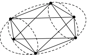
Let us take a look at Problem 1 from a geometric point of view. For simplicity, consider the noiseless case first. Here, a data matrix is just a separable matrix A. Separability implies that Ahas a factorization of the form (1). Under Assumption 1, conv(A) becomes an (r−1)-dimensional simplex in Rd. The left part of Figure 1 visualizes a separable data matrix. The white points are data points, and the black ones are basis vectors. The key observation is that the basis vectorsf1, . . . ,fr ofA correspond to the vertices of conv(A). This is due to separability. Therefore, if all vertices of conv(A) can be found, we can obtain the basis matrix F of A. This is not hard task, and we can design an efficient algorithm for doing it. But, if noise is added to a separable matrix, the task becomes hard. Let us suppose that the data matrix of Problem 1 is a noisy separable matrixAeof the formA+N.
The vertices of conv(Ae) do not necessarily match the basis vectors f1, . . . ,fr of A. The
right part of Figure 1 visualizes a noisy separable data matrix. This is the main reason why it is hard to identify the basis matrix from noisy separable one.
: Basis vector : Data point
Figure 1: Convex hull of a separable data matrix with r = 3 under Assumption 1. (Left) Noiseless case. (Right) Noisy case.
from a geometric point of view. Consider an (r −1)-dimensional simplex ∆ in Rr. Let
g1, . . . ,gr ∈ Rr be the vertices of ∆, and b1, . . . ,b` ∈ Rr be the points in ∆. We draw the MVEE centered at the origin for a set S = {±g1, . . . ,±gr,±b1, . . . ,±b`}. Then, the proposition says that the ellipsoid only touches the points±g1, . . . ,±gramong all the points in S. Therefore, the vertices of ∆ can be found by checking whether the points in S lie on the boundary of ellipsoid. We should mention that the convex hull of the points in
S becomes a full-dimensional crosspolytope in Rr. Figure 2 illustrates the MVEE for a crosspolytope in R3.
Figure 2: Minimum-volume enclosing ellipsoid for a full-dimensional crosspolytope inR3.
Under Assumption 1, the convex hull of a separable matrix A becomes an (r − 1)-dimensional simplex in Rd. Therefore, we rotate and embed the simplex in Rr by using an orthogonal transformation. Such a transformation can be obtained by singular value decomposition (SVD) of A.
sim-plex inRr. Next, it draws the MVEE centered at the origin for a setS={±p1, . . . ,±pm}, wherep1, . . . ,pm are the column vectors ofP, and outputs r points lying on the ellipsoid. We call the algorithmellipsoidal rounding, abbreviated as ER. The main computational costs of ER are in computing the SVD of A and the MVEE for S. The MVEE compu-tation can be formulated as a tractable convex optimization problem with m variables. A polynomial-time algorithm exists, and it is also known that a hybrid of the interior-point algorithm and cutting plane algorithm works efficiently in practice.
In later sections, we will see that ER algorithm works well even if noise is added. In particular, we show that ER correctly identifies the near-basis vectors of a noisy separable matrix if the noise is smaller than some level. We consider a situation in which the noise exceeds that level. In such a situation, the shape of crosspolytope formed by the data points is considerably perturbed by the noise, and it is possible that the MVEE touches many points. We thus need to select r points from the points on the boundary of the ellipsoid. In this paper, we perform existing algorithms such as SPA (Gillis and Vavasis, 2014) and XRAY (Kumar et al., 2013) to make the selection. Hence, ER works as a preprocessor which filters out basis vector candidates from data points and enhances the performance of existing algorithms.
2.3 Related Work
First, we will review the algorithms for NMF of general nonnegative matrices. There are an enormous number of studies. A commonly used approach is to formulate it as a nonconvex optimization problem and compute the local solution. Let A be a d-by-m nonnegative matrix, and consider an optimization problem with matrix variables F ∈ Rd×r and W ∈ Rr×m,
minimize||F W −A||2F subject to F ≥0 and W ≥0.
This is an intractable nonconvex optimization problem, and in fact, it was shown to be NP-hard by Vavasis (2009). Therefore, the research target is in how to compute the local solution efficiently. It is popular to use the block coordinate descent (BCD) algorithm for this purpose. The algorithm solves the problem by alternately fixing the variables F and
W. The problem obtained by fixing either of F and W becomes a convex optimization problem. The existing studies propose to use, for instance, the projected gradient algorithm (Lin, 2007) and its variant (Lee and Seung, 2001), active set algorithm (Kim and Park, 2008, 2011), and projected quasi-Newton algorithm (Gong and Zhang, 2012). It is reported that the BCD algorithm shows good performance on average in computing NMFs. However, its performance depends on how we choose the initial point for starting the algorithm. We refer the reader to Kim et al. (2014) for a survey on the algorithms for NMF.
Next, we will survey the algorithms that work on noisy separable matrices. Four types of algorithm can be found:
• Hottopixx (Bittorf et al., 2012; Gillis, 2013; Gillis and Luce, 2013). Let A
be a separable matrix of the form F(I,K)Π. Consider a matrixC such that
C =Π−1
I K 0 0
Π∈Rm×m.
It satisfies A = AC, and also, if the diagonal element is one, the position of its diagonal element indicates the index of basis vector in A. The algorithm models C
as the variable of an LP problem. It entails solving a single LP problem with m2
variables.
• SPA (Gillis and Vavasis, 2014). LetA be a separable matrix of sized-by-m, and
S be the set of the column vectors of A. The algorithm is based on the following observation. Under Assumption 1, the maximum of a convex function over the ele-ments in S is attained at the vertex of conv(A). The algorithm finds one element a
inS that maximizes a convex function, and then, projects all elements in S into the orthogonal space to a. This procedure is repeated untilr elements are found.
• XRAY (Kumar et al., 2013). The algorithm has a similar spirit as SPA, but it uses a linear function instead of a convex one. Let A be a separable matrix of size
d-by-mandS be the set of the column vectors ofA. LetIk be the index set obtained after the kth iteration. This is a subset of {1, . . . , m} with cardinality k. In the (k+ 1)th iteration, it computes a residual matrix R=A(Ik)X∗−A, where
X∗ = arg min
X≥0||A(Ik)X−A||
2 2,
and picks up one of the column vectors ri of R. Then, it finds one element from
S which maximizes a linear function having ri as the normal vector. Finally, Ik is updated by adding the index of the obtained element. This procedure is repeated until r indices are found. The performance of XRAY depends on how we select the column vector of the residual matrixR for making the linear function. Several ways of selection, called “rand”, “max”, “dist” and “greedy”, have been proposed by the authors.
The next section describes the properties of these algorithms.
2.4 Comparison with Existing Algorithm
We compare the correctness and robustness properties of ER with those of AGKM, Hot-topixx, SPA, and XRAY. ER is shown to have the two properties in Theorems 5 and 9. In particular, our robustness property in Theorem 9 states that ER correctly identifies the near-basis matrix of a noisy separable one Ae, and a robustness property with τ = 1 holds
if we set
= σ(1−µ)
4 (3)
and p= 2 under Assumption 1. Here,σ is the minimum singular value of the basis matrix
F of a separable one Ain the Ae, that is,σ =σr(F), and µisµ(K):
for a weight matrix K of A. Under Assumption 1-a, we have µ ≤ 1, and in particular, equality holds if and only if ki has only one nonzero element.
All four of the existing algorithms have been shown to have a correctness property, whereas every one except XRAY has a robustness property. Hottopixx is the most similar to ER. Bittorf et al. (2012) showed that it has the correctness and robustness with τ = 1 properties if one sets
= αmin{d0, α}
9(r+ 1) (4)
and p = 1 under simpliciality and other assumptions. Here, α and d0 are as follows. α is
the minimum value of δF(j) for j = 1, . . . , r, whereδF(j) denotes an `1-distance between
the jth column vector fj of F and the convex hull of the remaining column vectors in F.
d0 is the minimum value of ||ai−fj||1 for every isuch that ai is not a basis vector, and everyj= 1, . . . , r. The robustness of Hottopixx is further analyzed (Gillis, 2013; Gillis and Luce, 2013).
It can be interpreted that theof ER (3) is given by the multiplication of two parameters representing flatness and closeness of a given data matrix since σ measures the flatness of the convex hull of data points, and 1−µmeasures the closeness between basis vectors and data points. Intuitively, we may say that an algorithm becomes sensitive to noise when a data matrix has the following features; one is that the convex hull of data points is close to a flat shape, and another is that there are data points close to basis vectors. The of (3) well matches the intuition. We see a similar structure in theof Hottopixx (4) sinceα and
d0 respectively measure the flatness and closeness of a given data.
Compared with Hottopixx, the of ER (3) does not contain 1/r, and hence, it does not decrease asrincreases. However, Assumption 1-b of ER is stronger than the simpliciality of Hottopixx. In a practical implementation, ER can handle a large matrix, while Hottopixx may have limitations on the size of the matrix it can handle. Hottopixx entails solving an LP problem with m2 variables. In the NMFs arising in applications, m tends to be a large number. Although an LP is tractable, it becomes harder to solve as the size increases. Through experiments, we assessed the performance of Hottopixx with the CPLEX LP solver. The experiments showed that the algorithm had out of memory issues when m exceeded 2,000 with d = 100. Bittorf et al. (2012) proposed a parallel implementation to resolve these computational issues.
AGKM and SPA were shown to have a robustness property with τ ≥ 1 for some in Arora et al. (2012a) and Gillis and Vavasis (2014), respectively. In practical implemen-tations, SPA and XRAY are scalable to the problem size and experimentally show good robustness. Section 6 reports a numerical comparison of ER with SPA and XRAY.
3. Review of Formulation and Algorithm for MVEE Computation
We review the formulation for computing the MVEE for a set of points, and survey the existing algorithms for the computation.
(x−z)>L(x−z) = 1, we call it an active pointof the ellipsoid. In other words, an active point is one lying on the boundary of the ellipsoid.
The volume of the ellipsoid is given as c(d)/√detL, wherec(d) represents the volume of a unit ball in Rd and it is a real number depending on the dimension d. ER algorithm considers d-dimensional ellipsoids containing a set S of points in Rd, and in particular, finds the minimum volume ellipsoid centered at the origin. In this paper, such an ellipsoid is referred to as an origin-centered MVEE for short.
Now, we are ready to describe a formulation for computing the origin-centered MVEE for a set of points. For m pointsp1, . . . ,pm ∈Rd, let S ={±p1, . . . ,±pm}. The computation of the origin-centered MVEE forS is formulated as
Q(S) : minimize −log detL,
subject to hpip>i ,Li ≤1, i= 1, . . . , m,
L0,
where the matrix L of size dis the decision variable. The optimal solution L∗ of Qgives the origin-centered MVEE for S as E(L∗) = {x :x>L∗x ≤ 1}. We here introduce some terminology. An active point ofE(L∗) is a vector pi ∈Rd satisfying p>i L∗pi = 1. We call
pi an active point of Q(S), and the index i of pi an active index of Q(S). The ellipsoid
E(L∗) is centrally symmetric, and if a vector pi is an active point, so is −pi. The dual of
Qreads
Q∗(S) : maximize log det Ω(u),
subject to e>u= 1, u≥0,
where the vector u is the decision variable. Here, Ω :Rm → Sd is a linear function given as Ω(u) =Pm
i=1pip>i ui; equivalently, Ω(u) =Pdiag(u)P> forP = (p1, . . . ,pm)∈Rd×m. It follows from the Karush-Kuhn-Tucker (KKT) conditions for these problems that the optimal solutionL∗ ofQis represented by 1dΩ(u∗)−1 for the optimal solutionu∗ ofQ∗. We
make the following assumption to ensure the existence of an optimal solution ofQ.
Assumption 2 rank(P) =dfor P = (p1, . . . ,pm)∈Rd×m.
Later, the KKT conditions will play an important role in our discussion of the active points of Q. Here though, we will describe the conditions: L∗ ∈Sd is an optimal solution for Q and z∗ ∈Rm is the associated Lagrange multiplier vector if and only if there exist
L∗ ∈Sdand z∗ ∈
Rm such that
−(L∗)−1+ Ω(z∗) =0, (5)
zi∗(hpip>i ,L∗i −1) = 0, i= 1, . . . , m, (6)
hpip>i ,L
∗i ≤
1, i= 1, . . . , m, (7)
L∗ 0, (8)
zi∗ ≥0, i= 1, . . . , m. (9)
Many algorithms have been proposed for solving problems Q and Q∗. These can be
Frank-Wolfe algorithms) and interior-point algorithms. Below, we survey the studies on these two algorithms.
Khachiyan (1996) proposed a barycentric coordinate descent algorithm, which can be interpreted as a conditional gradient algorithm. He showed that the algorithm has a polynomial-time iteration complexity. Several researchers investigated and revised Khachiyan’s algorithm. Kumar and Yildirim (2005) showed that the iteration complex-ity of Khachiyan’s algorithm can be slightly reduced if it starts from a well-selected initial point. Todd and Yildirim (2007) and Ahipasaoglu et al. (2008) incorporated a step called as a Wolfe’s away-step. The revised algorithm was shown to have a polynomial-time iteration complexity and a linear convergence rate.
A dual interior-point algorithm was given by Vandenberghe et al. (1998). A primal-dual interior-point algorithm was given by Toh (1999), and numerical experiments showed that this algorithm is efficient and can provide accurate solutions. A practical algorithm was designed by Sun and Freund (2004) for solving large-scale problems. In particular, a hybrid of the interior-point algorithm and cutting plane algorithm was shown to be effi-cient in numerical experiments. For instance, the paper reported that the hybrid algorithm can solve problems with d= 30 and m = 30,000 in under 30 seconds on a personal com-puter. Tsuchiya and Xia (2007) considered generalized forms of Q and Q∗ and showed
that a primal-dual interior-point algorithm for the generalized forms has a polynomial-time iteration complexity.
Next, let us discuss the complexity of these two sorts of algorithms for Q and Q∗. In
each iteration, the arithmetic operations of the conditional gradient algorithms are less than those of the interior-point algorithms. Each iteration of a conditional gradient algorithm (Khachiyan, 1996; Kumar and Yildirim, 2005; Todd and Yildirim, 2007; Ahipasaoglu et al., 2008) requires O(md) arithmetic operations. On the other hand, assuming that the num-ber of data points m is sufficiently larger than the dimension of data points d, the main complexity of interior-point algorithms (Vandenberghe et al., 1998; Toh, 1999) comes from solving an m-by-msystem of linear equations in each iteration. The solution serves as the search direction for the next iteration. Solving these linear equations requiresO(m3) arith-metic operations. In practice, the number of iterations of conditional gradient algorithms is much larger than that of interior-point algorithms. Ahipasaoglu et al. (2008) reports that conditional gradient algorithms take several thousands iterations to solve problems such that d runs from 10 to 30 and m from 10,000 to 30,000. On the other hand, Sun and Freund (2004) reports that interior-point algorithms usually terminate after several dozen iterations and provide accurate solutions.
One of the concerns about interior-point algorithms is the computational cost of each iteration. It is possible to reduce the cost considerably by using a cutting plane strategy. A hybrid of interior-point algorithm and cutting plane algorithm has an advantage over conditional gradient algorithms. In fact, Ahipasaoglu et al. (2008) reports that the hybrid algorithm is faster than the conditional gradient algorithms and works well even on large problems. Therefore, we use the hybrid algorithm to solveQin our practical implementation of ER. The details are in Section 5.1.
“active set strategy”, since it might be confused with “active set algorithm” for solving a nonnegative least square problem.
4. Description and Analysis of the Algorithm
The ER algorithm is presented below. Throughout of this paper, we use the notationNto denote a set of nonnegative integer numbers.
Algorithm 1 Ellipsoidal Rounding (ER) for Problem 1
Input: M ∈Rd+×m andr ∈N. Output: I.
1: Compute the SVD of M, and construct the reduced matrix P ∈ Rr×m associated withr.
2: Let S = {±p1, . . . ,±pm} for the column vectors p1, . . . ,pm of P. Solve Q(S), and construct the active index setI.
Step 1 needs to be explained in detail. LetM be a noisy separable matrix of sized
-by-m. In general, the M is a full-rank due to the existence of a noise matrix. However, the rank is close torwhen the amount of noise is small, and in particular, it isrin the noiseless case. Accordingly, we construct a low-rank approximation matrix to M and reduce the redundancy in the space spanned by the column vectors of M.
We use an SVD for the construction of the low-rank approximation matrix. The SVD of M gives a decomposition of the form,
M =UΣV>.
Here,U andV ared-by-dand m-by-morthogonal matrices, respectively. In this paper, we call theU aleft orthogonal matrixof the SVD ofM. Lett= min{d, m}. Σ is a rectangular diagonal matrix consisting of the singular values σ1, . . . , σt ofM, and it is of the form,
Σ = diag(σ1, . . . , σt)∈Rd×m
withσ1≥ · · · ≥σt≥0. By choosing the topr singular values while setting the others to 0 in Σ, we construct
Σr= diag(σ1, . . . , σr,0, . . . ,0)∈Rd×m
and let
Mr=UΣrV>.
Mris the best rank-r approximation toM as measured by the matrix 2-norm and satisfies
||M −Mr||2 = σr+1 (see, for instance, Theorem 2.5.3 of Golub and Loan, 1996). By
applying the left orthogonal matrix U> toMr, we have
U>Mr=
P 0
∈Rd×m,
4.1 Correctness for a Separable Matrix
We analyze the correctness property of Algorithm 1. Let A be a separable matrix of size
d-by-m. Assume that Assumption 1 holds for A. We run Algorithm 1 for (A,rank(A)). Step 1 computes the reduced matrixP of A. Sincer = rank(A), we have A=Ar, where
Ar is the best rank-r approximation matrix to A. Let U ∈
Rd×d be the left orthogonal matrix of the SVD ofA. The reduced matrix P ∈Rr×m ofA is obtained as
P 0
= U>A
= U>F(I,K)Π. (10)
From the above, we see that
U>F =
G 0
∈Rd×m, where G∈Rr×r. (11)
Here, we have rank(G) =r since rank(F) =r by Assumption 1-b andU is an orthogonal matrix. By usingG, we rewriteP as
P = (G,GK)Π.
From Assumption 1-a, the column vectors ki of the weight matrix K ∈ Rr×` satisfy the conditions
||ki||1= 1 and ki ≥0, i= 1, . . . , `. (12) In Step 2, we collect the column vectors of P and construct a set S of them. Let
B =GK, and let gj and bi be the column vector ofG and B, respectively. S is a set of vectors ±g1, . . . ,±gr,±b1, . . . ,±b`. The following proposition guarantees that the active points of Q(S) are g1, . . . ,gr. We can see from (10) and (11) that the index set of the column vectors of Gis identical to that of of F. Hence, the basis matrixF of a separable oneA can be obtained by finding the active points ofQ(S).
Proposition 3 Let G∈Rr×r andB=GK ∈Rr×` forK ∈Rr×`. For the column vectors
gj and bi of G and B, respectively, let S = {±g1, . . .±gr,±b1, . . . ,±b`}. Suppose that
rank(G) = r and K satisfies the condition (12). Then, the active point set of Q(S) is
{g1, . . . ,gr}.
Proof We show that an optimal solution L∗ of Q(S) is (GG>)−1 and its associated Lagrange multiplier z∗ is (e;0), where e is an r-dimensional all-ones vector and 0 is an `-dimensional zero vector. Here, the Lagrange multipliers are one for the constraints
hgjg>j ,Li ≤1, and these are zero for hbib>i ,Li ≤1.
Since G is nonsingular, the inverse of GG> exists and it is positive definite. Now we check that L∗ = (GG>)−1 and z∗ = (e;0) satisfy the KKT conditions (5)-(9) for the problem. It was already seen that the conditions (5), (8), and (9) are satisfied. For the remaining conditions, we have
and
hbib>i ,(GG
>
)−1i = (B>(GG>)−1B)ii = (K>G>(GG>)−1GK)ii = ki>ki
≤ ||ki||2
1= 1. (14)
Here, (·)ii for a matrix denotes the (i, i)th element of the matrix. The inequality in (14) follows from condition (12). Also, the Lagrange multipliers are zero for the inequality constraints hbib>i ,(GG>)−1i ≤1. Thus, conditions (6) and (7) are satisfied. Accordingly, (GG>)−1 is an optimal solution of Q(S).
We can see from (13) that g1, . . . ,gr are the active points of the problem. Moreover, we may have equality in (14). In fact, equality holds if and only if ki has only one nonzero element. For suchki,bi=Gki coincides with some vector in g1, . . . ,gr.
From the above discussion, we can immediately notice that this proposition holds if for a matrix K∈Rr×`, the column vectorski satisfy
||ki||2<1, i= 1, . . . , m. (15)
Note that in contrast with condition (12), this condition does not require the matrix to be nonnegative.
Corollary 4 Proposition 3 holds even if we suppose thatK∈Rr×` satisfies condition (15),
instead of condition (12).
Note that this corollary is used to show the robustness of Algorithm 1 on a noisy separable matrix. The correctness of Algorithm 1 for a separable matrix follows from the above discussion and Proposition 3.
Theorem 5 Let A be a separable matrix. Assume that Assumption 1 holds for A. Then, Algorithm 1 for (A,rank(A))returns an index set I such that A(I) =F.
4.2 Robustness for a Noisy Separable Matrix
Next, we analyze the robustness property of Algorithm 1. Let A be a separable matrix of size d-by-m. Assume that Assumption 1 holds for A. Let Ae be a noisy separable matrix
of the form A+N. We run Algorithm 1 for (A,e rank(A)). Step 1 computes the reduced
matrix P of Ae. LetU ∈Rd×d be the left orthogonal matrix of the SVD of Ae, andAer be
For the reduced matrix P ofAe, we have
P 0
= U>Aer
= U>(Ae−Aer) (16)
= U>(A+N−Aer)
= U>(A+N) (17)
= U>((F,F K)Π+N)
= U>(F +N(1),F K+N(2))Π (18)
= U>(Fb,F Kb +Nc)Π. (19)
The following notation is used in the above: N =N−Aer in (17);N(1) and N(2) in (18)
are thed-by-randd-by-`submatrices ofN such thatNΠ−1 = (N(1),N(2));Fb =F+N(1)
and Nc=−N(1)K+N(2) in (19). This implies that
U>Fb=
b
G 0
, whereGb ∈Rr×r, (20)
and
U>Nc=
R 0
, whereR∈Rr×`. (21)
Hence, we can rewrite P as
P = (G,b GKb +R)Π.
e
A is represented by (2) as
e
A= (Fe,F Ke +Nf)Π,
whereFe andNfdenote F +N(1) and −N(1)K+N(2), respectively. From (16), we have
(G,b GKb +R)Π
0
=U>((Fe,F Ke +Nf)Π−Aer).
Therefore, the index set of the column vectors of Gb is identical to that of Fe. If all the
column vectors of Gb are found in P, we can identify Fe hidden in Ae.
In Step 2, we collect the column vectors of P and construct a setS of them. Let
b
B =GKb +R, (22)
and let gbj and bbi respectively be the column vectors of Gb and Bb. S is a set of vectors
±bg1, . . . ,±gbr,±bb1, . . . ,±bb`. We can see from Corollary 4 that, if rank(Gb) = r and bbi is
written as bbi =Gbkbi by using kbi ∈Rr with||kbi||2 <1, the active points of Q(S) are given
as the column vectorsbg1, . . . ,gbrofGb. Below, we examine the amount of noiseN such that
the conditions of Corollary 4 still hold.
Lemma 6 Let Ae=A+N ∈Rd×m. Then, |σi(Ae)−σi(A)| ≤ ||N||2 for each i= 1, . . . , t
Proof See Corollary 8.6.2 of Golub and Loan (1996).
Lemma 7 Let n=||N||2 and µ=µ(K). 7-a) The matrix N of (17) satisfies ||N||2 ≤2n.
7-b) The column vectors ri of matrixR of (21) satisfy ||ri||2≤2n(µ+ 1) for i= 1, . . . , m. 7-c) The singular values of matrix Gb of (20) satisfy |σi(Gb)−σi(F)| ≤2n for i= 1, . . . , r.
Proof 7-a) Since N =N −Aer,
||N||2 ≤ ||N||2+||Aer||2.
We have||Aer||2 ≤nsince||Aer||2 =σr+1(Ae) and from Lemma 6,|σr+1(Ae)−σr+1(A)| ≤n.
Therefore, ||N||2 ≤2n.
7-b) Let nbi be the column vector of the matrix Ncof (19). Since U>nbi = (ri;0) for an
orthogonal matrix U, we have ||nbi||2 =||ri||2. Therefore, we will evaluate ||nbi||2. Let ki
and n(2)i be the column vectors of K and N(2), respectively. Then,nbi can be represented
as−N(1)k
i+n(2)i . Thus, by Lemma 7-a, we have
||ri||2 =||nbi||2 ≤ ||N(1)||2||ki||2+||n(2)i ||2≤2n(µ+ 1).
7-c) Since U>Fb= (Gb;0) for an orthogonal matrix U, the singular values ofFb andGb
are identical. Also, sinceFb =F +N(1) and Lemma 6, we have
|σi(Gb)−σi(F)|=|σi(Fb)−σi(F)| ≤ ||N(1)||2 ≤2n.
The following lemma ensures that the conditions of Corollary 4 hold if the amount of noise is smaller than a certain level.
Lemma 8 Let Gb be the matrix of (20), and let bbi be the column vector of Bb of (22).
Suppose that ||N||2 < for = 14σ(1−µ) where σ =σr(F) and µ=µ(K). Then, 8-a) rank(Gb) =r.
8-b) bbi is represented as Gbkbi =bbi by usingkbi such that||bki||2<1.
In the proof below,n denotes||N||2.
Proof 8-a) From Lemma 7-c, the minimum singular value of Gb satisfies
σr(Gb) ≥ σ−2n
> σ−2= 1
The final inequality follows fromσ >0 due to Assumption 1-b. Hence, we have rank(Gb) =r.
8-b) Let ki and ri be the column vectors of K and R, respectively. Then, we have
b
bi =Gkb i+ri. Since Lemma 8-a guarantees that Gb has an inverse, it can be represented
asbbi=Gbkbi by kbi =ki+Gb−1ri. It follows from Lemmas 7-b and 7-c that
||bki||2 ≤ ||ki||2+||Gb−1||2||ri||2
≤ µ+2n(µ+ 1)
σ−2n .
Since n < 14σ(1−µ), we have||bki||2 <1.
The robustness of Algorithm 1 for a noisy separable matrix follows from the above discussion, Corollary 4, and Lemma 8.
Theorem 9 LetAebe a noisy separable matrix of the formA+N. Assume that Assumption
1 holds for the separable matrixAin Ae. Set = 14σ(1−µ) whereσ=σr(F) andµ=µ(K)
for the basis and weight matricesF andKofA. If||N||2< , Algorithm 1 for(A,e rank(A))
returns an index set I such that ||Ae(I)−F||2< .
In Theorem 9, letF∗=Ae(I), andW∗be an optimal solution of the convex optimization
problem,
minimize||Ae(I)X −A||e 2F subject to X ≥0,
where the matrix X of size r-by-m is the decision variable. Then, (F∗,W∗) serves as the NMF factor of Ae. It is possible to evaluate the residual error of this factorization in a
similar way to the proof of Theorem 4 by Gillis and Vavasis (2014).
Corollary 10 Let wi∗ and aei be the column vectors of W
∗ and
e
A, respectively. Then, ||F∗w∗
i −aei||2<2for i= 1, . . . , m.
Proof From Assumption 1-a, the column vectors wi of W satisfy ||wi||2 ≤ 1 for i =
1, . . . , m. Therefore, for i= 1, . . . , m,
||F∗w∗i −aei||2 ≤ ||F∗wi−aei||2
= ||F∗wi−F wi+F wi−ai−ni||2
= ||(F∗−F)wi−ni||2
≤ ||F∗−F||2||wi||2+||ni||2<2,
whereai and ni denote the ith column vector of Aand N, respectively.
5. Implementation in Practice
which the theorem is valid. In such a situation, the algorithm might generate more active points than hoped. Therefore, we need to add a selection step in whichr points are selected from the active points. Also, the number of active points depends on which dimension we choose in the computation of the reduced matrix P. Algorithm 1 computes the reduced matrix P of the data matrix and draws an origin-centered MVEE for the column vectors
p1, . . . ,pm of P. As we will see in Lemma 11, the number of active points depends on the dimension of p1, . . . ,pm. Therefore, we introduce an input parameter ρ to control the dimension. By taking account of these considerations, we design a practical implementation of Algorithm 1.
Algorithm 2 Practical Implementation of Algorithm 1
Input: M ∈Rd+×m, r∈N, and ρ∈N. Output: I.
1: Run Algorithm 1 for (M, ρ). LetJ be the index set returned by the algorithm.
2: If |J |< r, increase ρ by 1 and go back to Step 1. Otherwise, select r elements from
J and construct the set I of these elements.
One may wonder whether Algorithm 2 infinitely loops or not. In fact, we can show that under some conditions, infinite loops do not occur.
Lemma 11 For p1, . . . ,pm ∈ Rρ, let S = {±p1, . . . ,±pm}. Suppose that Assumption 2
holds. Then, Q(S) has at least ρ active points.
Proof Consider the KKT conditions (5)-(9) for Q(S). Condition (5) requires Ω(z∗) to be nonsingular. Since rank(P) =ρ from the assumption, at least ρ nonzerozi∗ exist. There-fore, we see from condition (6) that Q(S) has at leastρ active points.
Proposition 12 Suppose that we choose r such that r ≤ rank(M). Then, Algorithm 2 terminates after a finite number of iterations.
Proof For the active index setJ constructed in Step 1, Lemma 11 guarantees that|J | ≥ρ. The parameter ρ increases by 1 if |J | < r in Step 2 and can continue to increase up to
ρ = rank(M). Since r ≤ rank(M), it is necessarily to satisfy |J | ≥ ρ ≥ r after a finite number of iterations.
Proposition 12 implies that ρmay not be an essential input parameter since Algorithm 2 always terminates underr ≤rank(M) even if starting with ρ= 1.
5.1 Cutting Plane Strategy for Solving Q
LetS be a set of mpoints inRd. As mentioned in Section 3,O(m3) arithmetic operations are required in each iteration of an interior-point algorithm for Q(S). A cutting plane strategy is a way to reduce the number of points which we need to deal with in solving Q(S). The strategy was originally used by Sun and Freund (2004). In this section, we describe the details of our implementation.
The cutting plane strategy for solvingQhas a geometric interpretation. It is thought of that active points contribute a lot to the drawing the MVEE for a set of points but inactive points make less of a contribution. This geometric intuition can be justified by the following proposition. Let L be a d-by-d matrix. We use the notation δL(p) to denote hpp>,Li for an elementp∈Rd ofS.
Proposition 13 Let S¯ be a subset of S. If an optimal solution L¯∗ of Q( ¯S) satisfies
δL¯∗(p)≤1 for allp∈ S \S¯, then L¯∗ is an optimal solution of Q(S).
The proof is omitted since it is obvious. The proposition implies thatQ(S) can be solved by using its subset ¯S instead ofS. The cutting plane strategy offers a way of finding such a
¯
S, in which a smaller problemQ( ¯S) has the same optimal solution asQ(S). In this strategy, we first choose some points from S and construct a setS1 containing these points. LetSk be the set constructed in thekth iteration. In the (k+ 1)th iteration, we choose some points from S \ Sk and expandSk toSk+1 by adding these points toSk. Besides expanding, we also shrink Sk by discarding some points which can be regarded as useless for drawing the origin-centered MVEE. These expanding and shrinking phases play an important role in constructing a small set. Algorithm 3 describes a cutting plane strategy for solvingQ(S).
Algorithm 3 Cutting Plane Strategy for SolvingQ(S)
Input: S ={p1, . . . ,pm}.
Output: L∗.
1: Choose an initial setS1 from S and let k= 1.
2: Solve Q(Sk) and find the optimal solution Lk. IfδLk(p)≤1 holds for allp∈ S \ Sk, let L∗ =Lk, and stop.
3: Choose a subset F of Sk and a subset G of {p∈ S \ Sk :δ
Lk(p)>1}. UpdateSk as
Sk+1 = (Sk\ F)∪ G and increase k by 1. Then, go back to Step 2.
Now, we give a description of our implementation of Algorithm 3. To construct the initial set S1 in Step 1, our implementation employs the algorithm used in the papers (Kumar
and Yildirim, 2005; Todd and Yildirim, 2007; Ahipasaoglu et al., 2008). The algorithm constructs a set S1 by greedily choosing 2dpoints in a step-by-step manner such that the
convex hull is ad-dimensional crosspolytope containing as many points inS as possible. We refer the reader to Algorithm 3.1 of Kumar and Yildirim (2005) for the precise description. To shrink and expandSk in Step 3, we use a shrinking threshold parameterθ such that
θ <1, and an expanding size parameterηsuch that η≥1. These parameters are set before running Algorithm 3. For shrinking, we construct F ={p∈ Sk :δ
For expanding, we arrange the points of {p ∈ S \ Sk : δ
Lk(p) > 1} in descending order, as measured by δLk(·), and construct G by choosing the top (m−2d)/η points. If the set
{p ∈ S \ Sk : δ
Lk(p) > 1} has less than (m−2d)/η points, we choose all the points and constructG.
6. Experiments
We experimentally compared Algorithm 2 with SPA and the variants of XRAY. These two existing algorithms were chosen because their studies (Bittorf et al., 2012; Gillis and Luce, 2013; Kumar et al., 2013) report that they outperform AGKM and Hottopixx, and scale to the problem size. Two types of experiments were conducted: one is the evaluation for the robustness of the algorithms to noise on synthetic data sets, and the other is the application of the algorithms to clustering of real-world document corpora.
We implemented Algorithm 2, and three variants of XRAY, “max”, “dist” and “greedy”, in MATLAB. We put Algorithm 3 in Algorithm 2 so it would solve Q efficiently. The software package SDPT3 (Toh et al., 1999) was used for solvingQ(Sk) in Step 2 of Algorithm 3. The shrinking parameter θ and expanding size parameter η were set as 0.9999 and 5, respectively. The implementation of XRAY formulated the computation of the residual matrixR=A(Ik)X∗−Aas a convex optimization problem,
X∗= arg min
X≥0||A(Ik)X−A||
2
F.
For the implementation of SPA (Gillis and Vavasis, 2014), we used code from the first author’s website. Note that SPA and XRAY are sensitive to the normalization of the column vectors of the data matrix (see, for instance, Kumar et al., 2013), and for this reason, we used a data matrix whose column vectors were not normalized. All experiments were done in MATLAB on a 3.2 GHz CPU processor and 12 GB memory.
We will use the following abbreviations to represent the variants of algorithms. For instance, Algorithm 2 with SPA for an index selection of Step 2 is referred to as ER-SPA. Also, the variant of XRAY with “max” selection policy is referred to as XRAY(max).
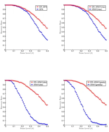
6.1 Synthetic Data
Experiments were conducted for the purpose of seeing how well Algorithm 2 could im-prove the robustness of SPA and XRAY to noise. Specifically, we compared it with SPA, XRAY(max), XRAY(dist), and XRAY(greedy). The robustness of algorithm was measured by a recovery rate. Let I be an index set of basis vectors in a noisy separable matrix, and I∗ be an index set returned by an algorithm. The recovery rate is the ratio given by
|I ∩ I∗|/ |I|.
We used synthetic data sets of the formF(I,K)Π+N with d= 250,m= 5,000, and
0 0.1 0.2 0.3 0.4 0.5 0 0.1 0.2 0.3 0.4 0.5 0.6 0.7 0.8 0.9 1
Noise Level (δ)
R ec o v er y R a te ER−SPA SPA
0 0.1 0.2 0.3 0.4 0.5
0 0.1 0.2 0.3 0.4 0.5 0.6 0.7 0.8 0.9 1
Noise Level (δ)
R ec o v er y R a te ER−XRAY(max) XRAY(max)
0 0.1 0.2 0.3 0.4 0.5
0 0.1 0.2 0.3 0.4 0.5 0.6 0.7 0.8 0.9 1
Noise Level (δ)
R ec o v er y R a te ER−XRAY(dist) XRAY(dist)
0 0.1 0.2 0.3 0.4 0.5
0 0.1 0.2 0.3 0.4 0.5 0.6 0.7 0.8 0.9 1
Noise Level (δ)
R ec o v er y R a te ER−XRAY(geedy) XRAY(greedy)
Recovery rate 100% 90% 80% 70%
ER-SPA 0.06 0.24 0.32 0.37
SPA 0.05 0.21 0.27 0.31
ER-XRAY(max) 0.06 0.24 0.32 0.37
XRAY(max) 0.05 0.21 0.27 0.31
ER-XRAY(dist) 0.07 0.23 0.29 0.36
XRAY(dist) 0.03 0.10 0.13 0.16
ER-XRAY(greedy) 0.07 0.23 0.29 0.35
XRAY(greedy) 0.00 0.08 0.12 0.14
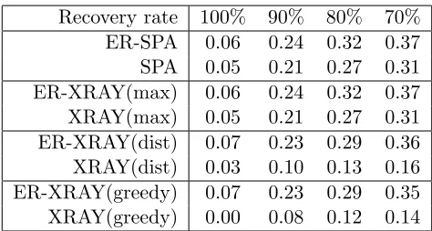
Table 1: Maximum values of noise levelδ for different recovery rates in percentage.
0 to 0.5 in 0.01 increments. A single data set consisted of 51 matrices with various amounts of noise, and we made 50 different data sets. Algorithm 2 was performed in the setting that
M is a matrix in the data set andr andρ are each 10.
Figure 3 depicts the average recovery rate on the 50 data sets for Algorithm 2, SPA and XRAY. Table 1 summarizes the maximum values of noise levelδ for different recovery rates in percentage. The noise level was measured by 0.01, and hence, for instance, the entry “0.00” at XRAY(greedy) for 100% recovery rate means that the maximum value is in the interval [0.00,0.01). We see from the figure that Algorithm 2 improved the recovery rates of the existing algorithms. In particular, the recovery rates of XRAY(dist) and XRAY(greedy) rapidly decrease as the noise level increases, but Algorithm 2 significantly improved them. Also, the figure shows that Algorithm 2 tended to slow the decrease in the recovery rate. We see from the table that Algorithm 2 is more robust to noise than SPA and XRAY.
Table 2 summarizes the average number of active points and elapsed time for 50 data sets taken by Algorithm 2 with δ = 0,0.25 and 0.5. We read from the table that the elapsed time increases with the number of active points. The average elapsed times of SPA, XRAY(max), XRAY(dist), and XRAY(greedy) was respectively 0.03, 1.18, 16.80 and 15.85 in seconds. Therefore, we see that the elapsed time of Algorithm 2 was within a reasonable range.
δ Active points Elapsed time (second)
ER-SPA ER-XRAY(max) ER-XRAY(dist) ER-XRAY(greedy)
0 10 1.05 1.07 1.07 1.07
0.25 12 3.08 3.10 3.10 3.10
0.5 23 4.70 4.71 4.71 4.71
Table 2: Average number of active points and elapsed time of Algorithm 2.
6.2 Application to Document Clustering
convex combination of several topic vectors w1, . . .wr. This type of generative model has been used in many papers (for instance, Xu et al., 2003; Shahnaz et al., 2006; Arora et al., 2012b, 2013; Ding et al., 2013; Kumar et al., 2013).
LetW be anr-by-mtopic matrix such thatw>1, . . . ,w>r are stacked from top to bottom and are of the form (w1;. . .;wr). The model allows us to write a document vector in the forma>i =fi>W by using a coefficient vectorfi ∈Rr such thate>fi= 1 andfi ≥0. This means that we haveA=F W for a document-by-word matrixA= (a1;. . .;ad)∈Rd+×m, a
coefficient matrixF = (f1;. . .;fd)∈Rd+×r, and a topic matrixW = (w1;. . .;wr)∈Rr+×m.
In the same way as the papers (Arora et al., 2012b, 2013; Ding et al., 2013; Kumar et al., 2013), we assume that a document-by-word matrix A is separable. This requires thatW
is of (I,K)Π, and it means that each topic has ananchor word. An anchor word is a word that is contained in one topic but not contained in the other topics. If an anchor word is found, it suggests that the associated topic exists.
Algorithms for Problem 1 can be used for clustering documents and finding topics for the above generative model. The algorithms for a document-word matrixAreturn an index set I. Let F =A(I). The row vector elementsfi1, . . . , fir of F can be thought of as the contribution rate of topics w1, . . . ,wr for generating a document ai. The highest value
fij∗ among the elements implies that the topicwj∗ contributes the most to the generation of document ai. Hence, we assign document ai to a cluster having the topic wj∗. There is an alternative to using F for measuring the contribution rates of the topics. Step 1 of Algorithm 1 produces a rank-r approximation matrix Ar to A as a by-product. Let
F0 =Ar(I), and use it as an alternative to F. We say that clustering withF is clustering with the original data matrix, and that clustering with F0 is clustering with a low-rank approximation data matrix.
Experiments were conducted in the purpose of investigating clustering performance of algorithms and also checking whether meaningful topics could be extracted. To investigate the clustering performance, we used only SPA since our experimental results implied that XRAY would underperform. We assigned the values of the document-word matrix on the basis of the tf-idf weighting scheme, for which we refer the reader to Manning et al. (2008), and normalized the row vectors to the unit 1-norm.
To evaluate the clustering performance, we measured the accuracy (AC) and normalized mutual information (NMI). These measures are often used for this purpose (see, for instance, Xu et al., 2003; Manning et al., 2008). Let Ω1, . . . ,Ωr be the manually classified classes and
C1, . . . ,Cr be the clusters constructed by an algorithm. Both Ωi and Cj are the subsets of the document set {a1, . . . ,am} such that each subset does not share any documents and the union of all subsets coincides with the document set. AC is computed as follows. First, compute the correspondence between classes Ω1, . . . ,Ωr and clusters C1, . . . ,Cr such that the total number of common documents Ωi ∩ Cj is maximized. This computation can be done by solving an assignment problem. After that, rearrange the classes and clusters in the obtained order and compute
1
d
r
X
k=1
This value is the AC for the clusters constructed by an algorithm. NMI is computed as
I(Ω,C)
1
2(E(Ω) +E(C)) .
I and E denote the mutual information and entropy for the class family Ω and cluster familyCwhere Ω ={Ω1, . . . ,Ωr} andC={C1, . . . ,Cr}. We refer the reader to Section 16.3 of Manning et al. (2008) for the precise forms of I and E.
Two document corpora were used for the clustering-performance evaluation: Reuters-21578 and 20 Newsgroups. These corpora are publicly available from the UCI Knowledge Discovery in Databases Archive (http://kdd.ics.uci.edu). In particular, we used the data preprocessing of Deng Cai, in which multiple classes are discarded. The data sets are available from the website (http://www.cad.zju.edu.cn/home/dengcai). The Reuters-21578 corpus consists of 21,578 documents appearing in the Reuters newswire in 1987, and these documents are manually classified into 135 classes. The text corpus is reduced by the preprocessing to 8,293 documents in 65 classes. Furthermore, we cut off classes with less than 5 documents. The resulting corpus contains 8,258 documents with 18,931 words in 48 classes, and the sizes of the classes range from 5 to 3,713. The 20 Newsgroups corpus consists of 18,846 documents with 26,213 words appearing in 20 different newsgroups. The size of each class is about 1,000.
We randomly picked some classes from the corpora and evaluated the clustering per-formance 50 times. Algorithm 2 was performed in the setting thatM is a document-word matrix and r and ρ each are the number of classes. In clustering with a low-rank ap-proximation data matrix, we used the rank-r approximation matrix to a document-word matrix.
AC NMI
Original Low-rank approx. Original Low-rank approx.
# Classes ER-SPA SPA ER-SPA SPA ER-SPA SPA ER-SPA SPA
6 0.605 0.586 0.658 0.636 0.407 0.397 0.532 0.466
8 0.534 0.539 0.583 0.581 0.388 0.387 0.491 0.456
10 0.515 0.508 0.572 0.560 0.406 0.393 0.511 0.475
12 0.482 0.467 0.532 0.522 0.399 0.388 0.492 0.469
Table 3: (Reuters-21578) Average AC and NMI of ER-SPA and SPA with the original data matrix and low-rank approximation data matrix.
AC NMI
Original Low-rank approx. Original Low-rank approx.
# Classes ER-SPA SPA ER-SPA SPA ER-SPA SPA ER-SPA SPA
6 0.441 0.350 0.652 0.508 0.314 0.237 0.573 0.411
8 0.391 0.313 0.612 0.474 0.306 0.242 0.555 0.415
10 0.356 0.278 0.559 0.439 0.291 0.228 0.515 0.397
12 0.319 0.240 0.517 0.395 0.268 0.205 0.486 0.372
Table 4: (20 Newsgroups) Average AC and NMI of ER-SPA and SPA with the original data matrix and low-rank approximation data matrix.
low-rank approximation data matrix. Table 4 indicates that ER-SPA outperformed SPA in AC and NMI on 20 Newsgroups.
Finally, we compared the topics obtained by ER-SPA and SPA. We used the BBC corpus of Greene and Cunningham (2006), which is available from the website (http:
//mlg.ucd.ie/datasets/bbc.html). The documents in the corpus have been subjected
by preprocessed such as stemming, stop-word removal, and low word frequency filtering. It consists of 2,225 documents with 9,636 words that appeared on the BBC news website in 2004-2005. The documents were news on 5 topics: “business”, “entertainment”, “politics”, “sport” and “tech”.
AC NMI
ER-SPA SPA ER-SPA SPA
0.939 0.675 0.831 0.472
Table 5: AC and NMI of ER-SPA and SPA with low-rank approximation data matrix for BBC.
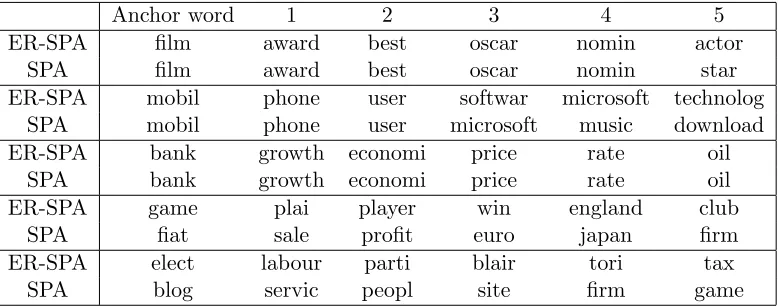
Anchor word 1 2 3 4 5
ER-SPA film award best oscar nomin actor
SPA film award best oscar nomin star
ER-SPA mobil phone user softwar microsoft technolog
SPA mobil phone user microsoft music download
ER-SPA bank growth economi price rate oil
SPA bank growth economi price rate oil
ER-SPA game plai player win england club
SPA fiat sale profit euro japan firm
ER-SPA elect labour parti blair tori tax
SPA blog servic peopl site firm game
Table 5 shows the ACs and NMIs of ER-SPA and SPA on the low-rank approximation data matrix for the BBC corpus. The table indicates that the AC and NMI of ER-SPA are higher than those of SPA. Table 6 summarizes the words in the topics obtained by ER-SPA and ER-SPA. The topics were computed by using a low-rank approximation data matrix. The table lists the anchor word and the 5 most frequent words in each topic from left to right. We computed the correspondence between topics obtained by ER-SPA and SPA and grouped the topics for each algorithm. Concretely, we measured the 2-norm of each topic vector and computed the correspondence by solving an assignment problem. We can see from the table that the topics obtained by these two algorithms are almost the same from the first to the third panel, and they seem to correspond to “entertainment”, “tech” and “business”. The topics in the fourth and fifth panels, however, are different. The topic in the fifth panel by ER-SPA seems to correspond to “politics”. In contrast, it is difficult to find the topic corresponding to “politics” in the panels by SPA. These show that ER-SPA could extract more recognizable topics than SPA.
Remark 14 Sparsity plays an important role in computing the SVD for a large document corpus. In general, a document-word matrix arising from a text corpus is quite sparse. Our implementation of Algorithm 2 used the MATLAB commandsvds that exploits the sparsity of a matrix in the SVD computation. The implementation could work on all data of 20 Newsgroups corpus, which formed a document-word matrix of size 18,846-by-26,213.
7. Concluding Remarks
We presented Algorithm 1 for Problem 1 and formally showed that it has correctness and robustness properties. Numerical experiments on synthetic data sets demonstrated that Algorithm 2, which is the practical implementation of Algorithm 1, is robustness to noise. The robustness of the algorithm was measured in terms of the recovery rate. The results indicated that Algorithm 2 can improve the recovery rates of SPA and XRAY. The algo-rithm was then applied to document clustering. The experimental results implied that it outperformed SPA and extracted more recognizable topics.
We will conclude by suggesting a direction for future research. Algorithm 2 needs to do two computations: one is the SVD of the data matrix and the other is the MVEE for a set of reduced-dimensional data points. It would be ideal to have a single computation that could be parallelized. The MVEE computation requires that the convex hull of data points is full-dimensional. Hence, the SVD computation should be carried out on data points. However, if we could devise an alternative convex set for MVEE, it would possible to avoid SVD computation. It would be interesting to investigate the possibility of algorithms that find near-basis vectors by using the other type of convex set for data points.
Acknowledgments
References
S. D. Ahipasaoglu, P. Sun, and M. J. Todd. Linear convergence of a modified Frank-Wolfe algorithm for computing minimum-volume enclosing ellipsoids. Optimization Methods and Software, 23(1):5–19, 2008.
S. Arora, R. Ge, R. Kannan, and A. Moitra. Computing a nonnegative matrix factorization – Provably. In Proceedings of the 44th Symposium on Theory of Computing (STOC), pages 145–162, 2012a.
S. Arora, R. Ge, and A. Moitra. Learning topic models – Going beyond SVD. InProceedings of the 2012 IEEE 53rd Annual Symposium on Foundations of Computer Science (FOCS), pages 1–10, 2012b.
S. Arora, R. Ge, Y. Halpern, D. Mimno, and A. Moitra. A practical algorithm for topic modeling with provable guarantees. In Proceedings of the 30th International Conference on Machine Learning (ICML), 2013.
V. Bittorf, B. Recht, C. Re, and J. A. Tropp. Factoring nonnegative matrices with linear programs. In Advances in Neural Information Processing Systems 25 (NIPS), pages 1223–1231, 2012.
A. Cichocki, R. Zdunek, A. H. Phan, and S. Amari. Nonnegative Matrix and Tensor Factorizations: Applications to Exploratory Multi-way Data Analysis and Blind Source Separation. Wiley, 2009.
W. Ding, M. H. Rohban, P. Ishwar, and V. Saligrama. Topic discovery through data dependent and random projections. In Proceedings of the 30th International Conference on Machine Learning (ICML), 2013.
D. Donoho and V. Stodden. When does non-negative matrix factorization give a correct decomposition into parts? In Advances in Neural Information Processing Systems 16 (NIPS), pages 1141–1148, 2003.
N. Gillis. Robustness analysis of Hottopixx, a linear programming model for factoring nonnegative matrices. SIAM Journal on Matrix Analysis and Applications, 34(3):1189– 1212, 2013.
N. Gillis and R. Luce. Robust near-separable nonnegative matrix factorization using linear optimization. arXiv:1302.4385v1, 2013.
N. Gillis and S. A. Vavasis. Fast and robust recursive algorithms for separable nonnegative matrix factorization. IEEE Transactions on Pattern Analysis and Machine Intelligence, 36(4):698–714, 2014.
G. H. Golub and C. F. Van Loan. Matrix Computation. The Johns Hopkins University Press, 3rd edition, 1996.
D. Greene and P. Cunningham. Practical solutions to the problem of diagonal dominance in kernel document clustering. In Proceedings of the 23th International Conference on Machine Learning (ICML), 2006.
L. G. Khachiyan. Rounding of polytopes in the real number model of computation. Math-ematics of Operations Research, 21(2):307–320, 1996.
H. Kim and H. Park. Non-negative matrix factorization based on alternating non-negativity constrained least squares and active set method. SIAM Journal on Matrix Analysis and Applications, 30(2):713–730, 2008.
H. Kim and H. Park. Fast nonnegative matrix factorization: An active-set-like method and comparisons. SIAM Journal on Scientific Computing, 33(6):3261–3281, 2011.
J. Kim, Y. He, and H. Park. Algorithms for nonnegative matrix and tensor factoriza-tions: a unified view based on block coordinate descent framework. Journal of Global Optimization, 58(2):285–319, 2014.
A. Kumar, V. Sindhwani, and P. Kambadur. Fast conical hull algorithms for near-separable non-negative matrix factorization. In Proceedings of the 30th International Conference on Machine Learning (ICML), 2013.
P. Kumar and E. A. Yildirim. Minimum-volume enclosing ellipsoids and core sets. Journal of Optimization Theory and Applications, 126(1), 2005.
D. D. Lee and H. S. Seung. Learning the parts of objects by non-negative matrix factoriza-tion. Nature, 401:788–791, 1999.
D. D. Lee and H. S. Seung. Algorithms for non-negative matrix factorization. InAdvances in Neural Information Processing Systems 13 (NIPS), pages 556–562, 2001.
C.-J. Lin. Projected gradient methods for non-negative matrix factorization. Neural Com-putation, 19(10):2756–2779, 2007.
C. D. Manning, P. Raghavan, and H. Schuetze. Introduction to Information Retrieval. Cambridge University Press, 2008.
L. Miao and H. Qi. Endmember extraction from highly mixed data using minimum volume constrained nonnegative matrix factorization. IEEE Transactions on Geoscience and Remote Sensing, 45(2):765–777, 2007.
J. M. P. Nascimento and J. M. B. Dias. Vertex component analysis: A fast algorithm to unmix hyperspectral data. IEEE Transactions on Geoscience and Remote Sensing, 43 (4):898–910, 2005.
F. Shahnaz, M. W. Berry, V. P. Pauca, and R. J. Plemmons. Document clustering using nonnegative matrix factorization. Information Processing and Management, 42(2):373– 386, 2006.
M. J. Todd and E. A. Yildirim. On Khachiyan’s algorithm for the computation of minimum-volume enclosing ellipsoids. Discrete Applied Mathematics, 155(13):1731–1744, 2007.
K.-C. Toh. Primal-dual path-following algorithms for determinant maximization problems with linear matrix inequalities. Computational Optimization and Applications, 14(3): 309–330, 1999.
K.-C. Toh, M. J. Todd, and R. H. T¨ut¨unc¨u. SDPT3 – a MATLAB software package for semidefinite programming. Optimization Methods and Software, 11:545–581, 1999.
T. Tsuchiya and Y. Xia. An extension of the standard polynomial-time primal-dual path-following algorithm to the weighted determinant maximization problem with semidefinite constraints. Pacific Journal of Optimization, 3(1):165–182, 2007.
L. Vandenberghe, S. Boyd, and S. P. Wu. Determinant maximization with linear matrix inequality constraints. SIAM Journal on Matrix Analysis and Applications, 19(2):499– 533, 1998.
S. A. Vavasis. On the complexity of nonnegative matrix factorization. SIAM Journal of Optimization, 20(3):1364–1377, 2009.