A Generalized Path Integral Control Approach to Reinforcement Learning

A Generalized Path Integral Control Approach

to Reinforcement Learning

Evangelos A.Theodorou [email protected]

Jonas Buchli [email protected]

Stefan Schaal∗ [email protected]

Department of Computer Science University of Southern California Los Angeles, CA 90089-2905, USA

Editor: Daniel Lee

Abstract

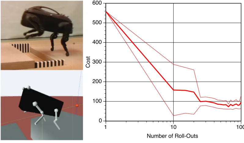
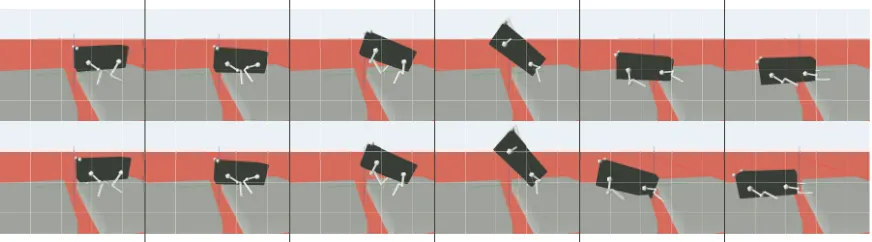
With the goal to generate more scalable algorithms with higher efficiency and fewer open parame-ters, reinforcement learning (RL) has recently moved towards combining classical techniques from optimal control and dynamic programming with modern learning techniques from statistical esti-mation theory. In this vein, this paper suggests to use the framework of stochastic optimal control with path integrals to derive a novel approach to RL with parameterized policies. While solidly grounded in value function estimation and optimal control based on the stochastic Hamilton-Jacobi-Bellman (HJB) equations, policy improvements can be transformed into an approximation problem of a path integral which has no open algorithmic parameters other than the exploration noise. The resulting algorithm can be conceived of as model-based, semi-model-based, or even model free, depending on how the learning problem is structured. The update equations have no danger of numerical instabilities as neither matrix inversions nor gradient learning rates are required. Our new algorithm demonstrates interesting similarities with previous RL research in the framework of probability matching and provides intuition why the slightly heuristically motivated probability matching approach can actually perform well. Empirical evaluations demonstrate significant per-formance improvements over gradient-based policy learning and scalability to high-dimensional control problems. Finally, a learning experiment on a simulated 12 degree-of-freedom robot dog illustrates the functionality of our algorithm in a complex robot learning scenario. We believe that Policy Improvement with Path Integrals (PI2) offers currently one of the most efficient, numeri-cally robust, and easy to implement algorithms for RL based on trajectory roll-outs.

Keywords: stochastic optimal control, reinforcement learning, parameterized policies

1. Introduction

While reinforcement learning (RL) is among the most general frameworks of learning control to cre-ate truly autonomous learning systems, its scalability to high-dimensional continuous stcre-ate-action systems, for example, humanoid robots, remains problematic. Classical value-function based meth-ods with function approximation offer one possible approach, but function approximation under the non-stationary iterative learning process of the value-function remains difficult when one exceeds about 5-10 dimensions. Alternatively, direct policy learning from trajectory roll-outs has recently made significant progress (Peters, 2007), but can still become numerically brittle and full of open

tuning parameters in complex learning problems. In new developments, RL researchers have started to combine the well-developed methods from statistical learning and empirical inference with clas-sical RL approaches in order to minimize tuning parameters and numerical problems, such that ulti-mately more efficient algorithms can be developed that scale to significantly more complex learning system (Dayan and Hinton, 1997; Koeber and Peters, 2008; Peters and Schaal, 2008c; Toussaint and Storkey, 2006; Ghavamzadeh and Yaakov, 2007; Deisenroth et al., 2009; Vlassis et al., 2009; Jetchev and Toussaint, 2009).

In the spirit of these latter ideas, this paper addresses a new method of probabilistic reinforce-ment learning derived from the framework of stochastic optimal control and path integrals, based on the original work of Kappen (2007) and Broek et al. (2008). As will be detailed in the sections be-low, this approach makes an appealing theoretical connection between value function approximation using the stochastic HJB equations and direct policy learning by approximating a path integral, that is, by solving a statistical inference problem from sample roll-outs. The resulting algorithm, called

Policy Improvement with Path Integrals (PI2), takes on a surprisingly simple form, has no open algorithmic tuning parameters besides the exploration noise, and it has numerically robust perfor-mance in high dimensional learning problems. It also makes an interesting connection to previous work on RL based on probability matching (Dayan and Hinton, 1997; Peters and Schaal, 2008c; Koeber and Peters, 2008) and motivates why probability matching algorithms can be successful.

This paper is structured into several major sections:

• Section 2 addresses the theoretical development of stochastic optimal control with path

in-tegrals. This is a fairly theoretical section. For a quick reading, we would recommend Sec-tion 2.1 for our basic notaSec-tion, and Table 1 for the final results. Exposing the reader to a sketch of the details of the derivations opens the possibility to derive path integral optimal control solutions for other dynamical systems than the one we address in Section 2.1.

The main steps of the theoretical development include:

– Problem formulation of stochastic optimal control with the stochastic

Hamilton-Jacobi-Bellman (HJB) equation

– The transformation of the HJB into a linear PDE

– The generalized path integral formulation for control systems with controlled and

un-controlled differential equations

– General derivation of optimal controls for the path integral formalism – Path integral optimal control applied to special cases of control systems

• Section 3 relates path integral optimal control to reinforcement learning. Several main issues

are addressed:

– Reinforcement learning with parameterized policies

– Dynamic Movement Primitives (DMP) as a special case of parameterized policies,

which matches the problem formulation of path integral optimal control.

– Derivation of Policy Improvement with Path Integrals (PI2), which is an application of path integral optimal control to DMPs.

• Section 5 illustrates several applications of PI2to control problems in robotics.

• Section 6 addresses several important issues and characteristics of RL with PI2.

2. Stochastic Optimal Control with Path Integrals

The goal in stochastic optimal control framework is to control a stochastic dynamical system while minimizing a performance criterion. Therefore, stochastic optimal control can be thought as a con-strained optimization problem in which the constrains corresponds to stochastic dynamical systems. The analysis and derivations of stochastic optimal control and path integrals in the next sections rely on the Bellman Principle of optimality (Bellman and Kalaba, 1964) and the HJB equation.

2.1 Stochastic Optimal Control Definition and Notation

For our technical developments, we will use largely a control theoretic notation from trajectory-based optimal control, however, with an attempt to have as much overlap as possible with the standard RL notation (Sutton and Barto, 1998). Let us define a finite horizon cost function for a

trajectoryτi (which can also be a piece of a trajectory) starting at time ti in state xti and ending at

time1tN

R(τi) =φtN+

Z tN

ti

rt dt, (1)

withφtN =φ(xtN)denoting a terminal reward at time tN and rt denoting the immediate cost at time

t. In stochastic optimal control (Stengel, 1994), the goal is to find the controls ut that minimize the value function:

V(xti) =Vti =min_u ti:tN

Eτi[R(τi)], (2)

where the expectation Eτi[.] is taken over all trajectories starting at xti. We consider the rather

general class of control systems:

˙xt=f(xt,t) +G(xt) (ut+εt) =ft+Gt(ut+εt), (3)

with xt∈ℜn×1denoting the state of the system, Gt =G(xt)∈ℜn×pthe control matrix, ft =f(xt)∈

ℜn×1 _{the passive dynamics, u}

t ∈ℜp×1the control vector andεt ∈ℜp×1Gaussian noise with

vari-anceΣε. As immediate cost we consider

rt=r(xt,ut,t) =qt+ 1

2u

T

t Rut, (4)

where qt =q(xt,t)is an arbitrary state-dependent cost function, and R is the positive semi-definite

weight matrix of the quadratic control cost. The stochastic HJB equation (Stengel, 1994; Fleming and Soner, 2006) associated with this stochastic optimal control problem is expressed as follows:

−∂tVt =min u

rt+ (∇xVt)TFt+ 1

2trace (∇xxVt)GtΣεG T t

, (5)

1. If we need to emphasize a particular time, we denote it by ti, which also simplifies a transition to discrete time

notation later. We use t without subscript when no emphasis is needed when this “time slice” occurs, t0for the start

where Ft is defined as Ft =f(xt,t) +G(xt)ut. To find the minimum, the cost function (4) is inserted into (5) and the gradient of the expression inside the parenthesis is taken with respect to controls u and set to zero. The corresponding optimal control is given by the equation:

u(xt) =ut =−R−1GtT(∇xtVt).

Substitution of the optimal control above, into the stochastic HJB (5), results in the following nonlinear and second order Partial Differential Equation (PDE):

−∂tVt=qt+ (∇xVt)Tft− 1 2(∇xVt)

T_G

tR−1GTt (∇xVt) + 1

2trace (∇xxVt)GtΣεG T t

.

The ∇x and∇xxsymbols refer to the Jacobian and Hessian, respectively, of the value function

with respect to the state x, while∂t is the partial derivative with respect to time. For notational

compactness, we will mostly use subscripted symbols to denote time and state dependencies, as introduced in the equations above.

2.2 Transformation of HJB into a Linear PDE

In order to find a solution to the PDE above, we use a exponential transformation of the value function:

Vt =−λlogΨt.

Given this logarithmic transformation, the partial derivatives of the value function with respect to time and state are expressed as follows:

∂tVt =−λ 1

Ψt

∂tΨt,

∇xVt =−λ 1

Ψt

∇xΨt,

∇xxVt =λ 1

Ψ2

t

∇xΨt ∇xΨTt −λ 1

Ψt

∇xxΨt.

Inserting the logarithmic transformation and the derivatives of the value function we obtain:

λ Ψt

∂tΨt =qt−

λ Ψt

(∇xΨt)Tft−

λ2

2Ψ2t

(∇xΨt)TGtR−1GTt (∇xΨt) + 1

2trace(Γ), (6)

where the termΓis expressed as:

Γ=

λ 1 Ψ2

t

∇xΨt ∇xΨTt −λ 1

Ψt

∇xxΨt

GtΣεGTt .

The trace ofΓis therefore:

trace(Γ) =λ 1

Ψ2trace ∇xΨ

T

t GtΣεGt∇xΨt

−λ_Ψ1

t

trace ∇xxΨtGtΣεGtT

Comparing the underlined terms in (6) and (7), one can recognize that these terms will cancel

under the assumption ofλR−1=Σε, which implies the simplification:

λGtR−1GtT=GtΣεGTt =Σ(xt) =Σt. (8) The intuition behind this assumption (cf. also Kappen, 2007; Broek et al., 2008) is that, since the weight control matrix R is inverse proportional to the variance of the noise, a high variance control input implies cheap control cost, while small variance control inputs have high control cost. From a control theoretic stand point such a relationship makes sense due to the fact that under a large disturbance (= high variance) significant control authority is required to bring the system back to a desirable state. This control authority can be achieved with corresponding low control cost in R.

With this simplification, (6) reduces to the following form

−∂tΨt=− 1

λqtΨt+fTt (∇xΨt) + 1

2trace (∇xxΨt)GtΣεG T t

, (9)

with boundary condition: ΨtN =exp −

1

λφtN

. The partial differential equation (PDE) in (9) corre-sponds to the so called Chapman Kolmogorov PDE, which is of second order and linear. Analytical solutions of (9) cannot be found in general for general nonlinear systems and cost functions. How-ever, there is a connection between solutions of PDEs and their representation as stochastic differ-ential equation (SDEs), that is mathematically expressed by the Feynman-Kac formula (Øksendal, 2003; Yong, 1997). The Feynman-Kac formula (see appendix B) can be used to find distributions of random processes which solve certain SDEs as well as to propose numerical methods for solving certain PDEs. Applying the Feynman-Kac theorem, the solution of (9) is:

Ψti =Eτi

ΨtNe

−R_titN 1

λqtdt_=Eτi

exp

−1_λφtN−

1

λ

Z tN

ti qt dt

. (10)

Thus, we have transformed our stochastic optimal control problem into the approximation prob-lem of a path integral. With a view towards a discrete time approximation, which will be needed for numerical implementations, the solution (10) can be formulated as:

Ψti= lim

dt→0

Z

p(τi|xi)exp "

−1_λ φtN+

N−1

∑

qtjdt

!#

dτi, (11)

where τi = (xti, ...,xtN) is a sample path (or trajectory piece) starting at state xti and the term

p(τi|xi)is the probability of sample pathτi conditioned on the start state xti. Since Equation (11)

provides the exponential cost to go Ψti in state xti, the integration above is taken with respect to

sample pathsτi = (xti,xti+1, ...,xtN). The differential term dτi is defined as dτi= (dxti, ...,dxtN).

Evaluation of the stochastic integral in (11) requires the specification of p(τi|xi), which is the topic

of our analysis in the next section.

2.3 Generalized Path Integral Formulation

To develop our algorithms, we will need to consider a more general development of the path integral approach to stochastic optimal control than presented in Kappen (2007) and Broek et al. (2008). In particular, we have to address that in many stochastic dynamical systems, the control transition

non-directly actuated parts. Since only some of the states are directly controlled, the state vector

is partitioned into x= [x(m)T x(c)T]T _{with x}(m)_∈ℜk×1 _{the non-directly actuated part and x}(c)_∈

ℜl×1_{the directly actuated part. Subsequently, the passive dynamics term and the control transition}

matrix can be partitioned as ft = [f(tm)

T

f(tc) T

]T _{with f}

m∈ℜk×1, fc∈ℜl×1and Gt= [0k_×p G(tc)

T ]T

with G(tc)∈ℜl×p. The discretized state space representation of such systems is given as:

xti+1=xti+ftidt+Gti

utidt+ √

dtεti

,

or, in partitioned vector form:

xt(im+1)

x(tic+)1 !

= x

(m)

ti x(tic)

! + f

(m)

ti f(tic)

!

dt+ 0k×p

G(_tic)

!

utidt+ √

dtεti

. (12)

Essentially the stochastic dynamics are partitioned into controlled equations in which the state

x(_tic₊)₁ is directly actuated and the uncontrolled equations in which the state x_t(_im₊₁)is not directly

actu-ated. Since stochasticity is only added in the directly actuated terms(c) of (12), we can develop

p(τi|xi)as follows.

p(τi|xti) = p(τi+1|xti)

= p(xtN, ...,xti+1|xti)

= ΠN_j=−_i1p xtj+1|xtj

,

where we exploited the fact that the start state xti of a trajectory is given and does not contribute

to its probability. For systems where the control has lower dimensionality than the state (12), the

transition probabilities p xtj+1|xtj

are factorized as follows:

p xtj+1|xtj

= p

xt(mj+)1|xtj

·p

x(tjc+)1|xtj

= p

x_t(m_j+)_1|x_t(_jm),x_t(c_j)

·p

x_t(_jc₊)_1|x_t(_jm),x(_tjc)

∝ p

xt(cj+)1|xtj

, (13)

where we have used the fact that p

xt(im+1)|x

(m)

ti ,x

(c)

ti

is the Dirac delta function, since x(tmj+)1 can be

computed deterministically from x_t(m_j ),x_t(c_j). For all practical purposes,2_{the transition probability of}

the stochastic dynamics is reduced to the transition probability of the directly actuated part of the state:

p(τi|xti) =Π

N−1

j=i p xtj+1|xtj

∝ Π_N−1 j=i p

x(_tjc₊)_1|xtj

. (14)

Since we assume that the noise ε is zero mean Gaussian distributed with varianceΣε, where

Σε∈ℜl×l_{, the transition probability of the directly actuated part of the state is defined as:}3

p

x(tcj+)1|xtj

= 1

(2π)l_{· |}Σ tj|

1/2exp − 1 2

w w wx

(c)

tj+1−x

(c)

tj −f

(c)

tj dt

w w w

2 Σ−1

t j

!

, (15)

2. The delta functions will all integrate to 1 in the path integral.

3. For notational simplicity, we write weighted square norms (or Mahalanobis distances) as vTMv=kvk2

where the covarianceΣtj ∈ℜ

l×l _{is expressed as Σ}

tj =G

(c)

tj ΣεG

(c)

tj

T

dt. Combining (15) and (14)

results in the probability of a path expressed as:

p(τi|xti)∝

1

ΠN−1

j=i (2π)lkΣtj|

1/2exp − 1 2

N−1

∑

w w wx

(c)

tj+1−x

(c)

tj −f

(c)

tj dt

w w w

2 Σ−1

t j

!

.

Finally, we incorporate the assumption (8) about the relation between the control cost and the

vari-ance of the noise, which needs to be adjusted to the controlled space as Σtj =G

(c)

tj ΣεG

(c)

tj

T

dt =

λG(c)

tj R− 1_G(c)

tj

T

dt=λHtjdt with Htj =G

(c)

tj R− 1_G(c)

tj

T

. Thus, we obtain:

p(τi|xti)∝

1

ΠN−1

j=i (2π)l|Σtj|

1/2exp 

−

1

2λ

N−1

∑

w w w w w

x(tcj+)1−x

(c)

tj

dt −f

(c)

tj w w w w w 2

H−_{t j}1

dt



.

With this formulation of the probability of a trajectory, we can rewrite the the path integral (11) as:

Ψti = lim

dt→0

Z exp



−_λ1 

φ_tN+∑N_j=−_i1q_tjdt+1₂∑N_j=−_i1 w w w w

x(_{t j}c₊)₁−x_{t j}(c)

dt −f

(c)

tj w w w w 2

H−_{t j}1

dt



 



ΠN−1

j=i (2π)l/2|Σtj|1/2

dτ

(c)

i

= lim dt→0

Z ₁

D(τi) exp

−_λ1S(τi

dτ(c)

i , (16)

where, we defined

S(τi) =φtN+

N−1

∑

qtjdt+

1 2

N−1

∑

w w w w w

x(tcj+)1−x

(c)

tj

dt −f

(c)

tj w w w w w 2

H−_{t j}1

dt,

and

D(τi) =ΠNj=−i1

(2π)l/2_|Σtj| 1/2_.

Note that the integration is over dτ(_ic)=dx(tic), ...,dx

(c)

tN

, as the non-directly actuated states can be integrated out due to the fact that the state transition of the non-directly actuated states is deterministic, and just added Dirac delta functions in the integral (cf. Equation (13)). Equation (16) is written in a more compact form as:

Ψti = lim

dt→0

Z exp

−_λ1S(τi)−log D(τi)

dτ(c)

i

= lim dt_→0

Z exp

−_λ1Z(τi)

dτ(c)

i , (17)

where Z(τi) =S(τi) +λlog D(τi). It can be shown that this term is factorized in path dependent

Z(τi) =S˜(τi) +

λ(N₋i)l

2 log(2πdtλ),

where ˜S(τi) =S(τi) +λ₂∑Nj=−i1log|Htj|. This formula is a required step for the derivation of

optimal controls in the next section. The constant term λ(N₂−i)llog(2πdtλ) can be the source of

numerical instabilities especially in cases where fine discretization dt of stochastic dynamics is required. However, in the next section, and in a great detail in Appendix A, lemma 1, we show how this term drops out of the equations.

2.4 Optimal Controls

For every moment of time, the optimal controls are given as uti =−R−

1_GT

ti(∇xtiVti). Due to the

exponential transformation of the value function, the equation of the optimal controls can be written as

uti =λR− 1_G

ti ∇x_tiΨti

Ψti .

After substitutingΨti with (17) and canceling the state independent terms of the cost we have:

uti = lim

dt→0





λR

−1_GT ti

∇_x(c) ti

R

e−1λS˜(τi)dτ(c)

i

R

e−1λS˜(τi)dτ(c)

i



 ,

Further analysis of the equation above leads to a simplified version for the optimal controls as

uti =

R

P(τi)uL(τi)dτ( c)

i , (18)

with the probability P(τi)and local controls uL(τi)defined as

P(τi) = e −1_λS˜(τi)

R e−1λS˜(τi)

dτi

(19)

uL(τi) =−R−1G(tic)

T _lim dt→0

∇_x(c) ti

˜

S(τi)

.

The path cost ˜S(τi)is a generalized version of the path cost in Kappen (2005a) and Kappen (2007),

which only considered systems with state independent control transition4 Gti. To find the local

controls uL(τi)we have to calculate the limdt→0∇_x(c)

ti

˜

S(τi). Appendix A and more precisely lemma

2 shows in detail the derivation of the final result:

lim dt→0

∇_x(c) ti

˜

S(τi)

=₋H−_ti1

G_t(_ic)εti−bti

,

where the new term bti is expressed as bti=λHtiΦti andΦti ∈ℜ

l×1_{is a vector with the j}th_element

defined as:

(Φti)j= 1 2trace

H_t−_i1

∂_[x(c) ti ]jHti

.

4. More precisely if G(tic)=G

(c)_{then the term}λ

2∑

N−1

The local control can now be expressed as:

uL(τi) =R−1G(tic)

T_H−1

ti

Gt(ic)εti−bti

,

By substituting Hti =G

(c)

ti R− 1_G(c)

ti

T _{in the equation above, we get our main result for the local}

controls of the sampled path for the generalized path integral formulation:

uL(τi) =R−1Gt(ic)

T_G(c)

ti R− 1_G(c)

ti

T−1_G(c)

ti εti−bti

. (20)

The equations in boxes (18), (19) and (20) form the solution for the generalized path integral stochastic optimal control problem. Given that this result is of general value and constitutes the foundation to derive our reinforcement learning algorithm in the next section, but also since many other special cases can be derived from it, we summarized all relevant equations in Table 1.

The Given components of Table 1 include a model of the system dynamics, the cost function,

knowledge of the system’s noise process, and a mechanism to generate trajectoriesτi. It is important

to realize that this is a model-based approach, as the computations of the optimal controls requires

knowledge ofεi. εi can be obtained in two ways. First, the trajectoriesτi can be generated purely

in simulation, where the noise is generated from a random number generator. Second, trajectories

could be generated by a real system, and the noiseεi would be computed from the difference

be-tween the actual and the predicted system behavior, that is, G(tic)εi =˙xti−ˆ˙xti = ˙xti−(fti+Gtiuti).

Computing the prediction ˆ˙xti also requires a model of the system dynamics.

Previous results in Kappen (2005a), Kappen (2007), Kappen (2005b) and Broek et al. (2008) are special cases of our generalized formulation. In the next section we show how our generalized formulation is specialized to different classes of stochastic dynamical systems and we provide the corresponding formula of local controls for each class.

2.5 Special Cases

The purpose of this section is twofold. First, it demonstrates how to apply the path integral approach to specialized forms of dynamical systems, and how the local controls in (20) simplify for these cases. Second, this section prepares the special case which we will need for our reinforcement learning algorithm in Section 3.

2.5.1 SYSTEMSWITHONEDIMENSIONALDIRECTLYACTUATEDSTATE

The generalized formulation of stochastic optimal control with path integrals in Table 1 can be applied to a variety of stochastic dynamical systems with different types of control transition matri-ces. One case of particular interest is where the dimensionality of the directly actuated part of the state is 1D, while the dimensionality of the control vector is 1D or higher dimensional. As will be seen below, this situation arises when the controls are generated by a linearly parameterized

func-tion approximator. The control transifunc-tion matrix thus becomes a row vector G_t(_ic)=g_t(_ic)T _∈ℜ1×p.

According to (20), the local controls for such systems are expressed as follows:

uL(τi) =

R−1g(tic) g(tic)TR−

1_g(c)

ti

g(_tic)Tεti−bti

• Given:

– The system dynamics ˙xt=ft+Gt(ut+εt)(cf. 3)

– The immediate cost rt =qt+1₂utTRut (cf. 4)

– A terminal cost termφtN (cf. 1)

– The varianceΣεof the mean-zero noiseεt

– Trajectory starting at tiand ending at tN:τi= (xti, ...,xtN)

– A partitioning of the system dynamics into(c) controlled and(m) uncontrolled

equa-tions, where n=c+m is the dimensionality of the state xt (cf. Section 2.3)

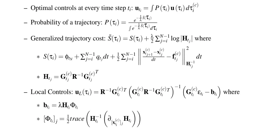
• Optimal Controls:

– Optimal controls at every time step ti: uti=

R

P(τi)u(τi)dτ(ic)

– Probability of a trajectory: P(τi) = e −1_λS˜(τi)

R e−λ1S˜(τi)

dτi

– Generalized trajectory cost: ˜S(τi) =S(τi) +λ₂∑Nj=−i1log|Htj|where ∗ S(τi) =φtN+∑

N−1

j=i qtjdt+ 1 2∑

N−1

j=i w w w w

x(_{t j}c₊) 1−x

(c) t j

dt −f

(c)

tj

w w w w

2

H−_{t j}1

dt

∗ Htj=G

(c)

tj R− 1_G(c)

tj

T

– Local Controls: uL(τi) =R−1G(tic)

T_G(c) ti R−

1_G(c)

ti

T−1_G(c) ti εti−bti

where

∗ bti=λHtiΦti ∗ [Φti]j=12trace

H−_ti1

∂_[x(c) ti ]jHti

Table 1: Summary of optimal control derived from the path integral formalizm.

Since the directly actuated part of the state is 1D, the vector xt(ic)collapses into the scalar x

(c)

ti

which appears in the partial differentiation above. In the case that g(tic)does not depend on x

(c)

ti , the

differentiation with respect to x(_tic)results to zero and the the local controls simplify to:

uL(τi) =

R−1g(tic)g

(c)T ti gt(ic)TR−

1_g(c)

ti εti.

2.5.2 SYSTEMS WITHPARTIALLYACTUATEDSTATE

The generalized formula of the local controls (20) was derived for the case where the control

transi-tion matrix is state dependent and its dimensionality is G(tc)∈ℜl×pwith l<n and p the

and robotic applications that belong into this general class. More precisely, for systems having a

state dependent control transition matrix that is square (G_t(_ic)_∈ℜl×l with l=p) the local controls

based on (20) are reformulated as:

uL(τi) =εti−G

(c)

ti

−1

bti. (21)

Interestingly, a rather general class of mechanical systems such as rigid-body and multi-body dynamics falls into this category. When these mechanical systems are expressed in state space

formulation, the control transition matrix is equal to rigid body inertia matrix G(_tic)=M(θti)

(Sci-avicco and Siciliano, 2000). Future work will address this special topic of path integral control for multi-body dynamics.

Another special case of systems with partially actuated state is when the control transition matrix

is state independent and has dimensionality Gt(c)=G(c)∈ℜl×p. The local controls, according to

(20), become:

uL(τi) =R−1G(c)

T

G(c)R−1G(c)T

−1

G(c)εti. (22)

If G_t(_ic)is square and state independent, G_t(_ic)=G(c)_∈ℜl×l, we will have:

uL(τi) =εti. (23)

This special case was explored in Kappen (2005a), Kappen (2007), Kappen (2005b) and Broek et al. (2008). Our generalized formulation allows a broader application of path integral control in areas like robotics and other control systems, where the control transition matrix is typically partitioned into directly and non-directly actuated states, and typically also state dependent.

2.5.3 SYSTEMS WITHFULLYACTUATEDSTATESPACE

In this class of stochastic systems, the control transition matrix is not partitioned and, therefore, the control u directly affects all the states. The local controls for such systems are provided by simply

substituting G(tic)∈ℜ

n×p_{in (20) with G}

ti∈ℜ

n×n_{. Since G}

ti is a square matrix we obtain:

uL(τi) =εti−G− 1

ti bti,

with bti =λHtiΦti and

(Φti)j= 1 2trace

H−_ti1

∂(x_ti)jHti

,

where the differentiation is not taken with respect to(x(_tic))jbut with respect to the full state(xti)j.

For this fully actuated state space, there are subclasses of dynamical systems with square and/or state independent control transition matrix. The local controls for these cases are found by just

substituting G(tic)with Gti in (21), (22) and (23).

3. Reinforcement Learning with Parameterized Policies

to learn compact policy representations, for example, with neural networks as in the early days of machine learning (Miller et al., 1990), or with general parameterizations (Peters, 2007; Deisenroth et al., 2009). Parameterized policies have much fewer parameters than the classical time-indexed approach of optimal control, where every time step has it own set of parameters, that is, the optimal controls at this time step. Usually, function approximation techniques are used to represent the op-timal controls and the open parameters of the function approximator become the policy parameters. Function approximators use a state representation as input and not an explicit time dependent rep-resentation. This representation allows generalization across states and promises to achieve better generalization of the control policy to a larger state space, such that policies become re-usable and do not have to be recomputed in every new situation.

The path integral approach from the previous sections also follows the classical time-based optimal control strategy, as can be seen from the time dependent solution for optimal controls in (33). However, a minor re-interpretation of the approach and some small mathematical adjustments allow us to carry it over to parameterized policies and reinforcement learning, which results in a

new algorithm called Policy Improvement with Path Integrals (PI2).

3.1 Parameterized Policies

We are focusing on direct policy learning, where the parameters of the policy are adjusted by a learning rule directly, and not indirectly as in value function approaches of classical reinforcement learning (Sutton and Barto, 1998)—see Peters (2007) for a discussion of pros and cons of direct vs. indirect policy learning. Direct policy learning usually assumes a general cost function (Sutton et al., 2000; Peters, 2007) in the form of

J(x0) =

Z

p(τ0)R(τ0)dτ0, (24)

which is optimized over states-action trajectories5τ0= (xt0,at0, ...,xtN). Under the first order Markov

property, the probability of a trajectory is

p(τi) =p(xti)Π

N−1

j=i p(xtj+1|xtj,atj)p(atj|xtj).

Both the state transition and the policy are assumed to be stochastic. The particular formulation of the stochastic policy is a design parameter, motivated by the application domain, analytical con-venience, and the need to inject exploration during learning. For continuous state action domains, Gaussian distributions are most commonly chosen (Gullapalli, 1990; Williams, 1992; Peters, 2007). An interesting generalized stochastic policy was suggested in Rueckstiess et al. (2008) and applied

in Koeber and Peters (2008), where the stochastic policy p(ati|xti)is linearly parameterized as:

ati =g

T

ti(θ+εti), (25)

with gti denoting a vector of basis functions andθthe parameter vector. This policy has state

de-pendent noise, which can contribute to faster learning as the signal-to-noise ratio becomes adaptive

since it is a function of gti. It should be noted that a standard additive-noise policy can be expressed

in this formulation, too, by choosing one basis function(gti)j=0. For Gaussian noiseεthe

proba-bility of an action is p(ati|xti) =N θ

T_g ti,Σti

withΣti=g

T

tiΣεgti. Comparing the policy formulation

5. We use atto denote actions here in order to avoid using the symbol u in a conflicting way in the equations below, and

in (25) with the control term in (3), one recognizes that the control policy formulation (25) should fit into the framework of path integral optimal control.

3.2 Generalized Parameterized Policies

Before going into more detail of our proposed reinforcement learning algorithm, it is worthwhile

contemplating what the action at actually represents. In many applications of stochastic optimal

control there are three main problems to be considered: i) trajectory planning, ii) feedforward con-trol, and iii) feedback control. The results of optimization could thus be an optimal kinematic trajectory, the corresponding feedforward commands to track the desired trajectory accurately in face of the system’s nonlinearities, and/or time varying linear feedback gains (gain scheduling) for a negative feedback controller that compensates for perturbations from accurate trajectory tracking. There are very few optimal control algorithms which compute all three issues simultaneously, such as Differential Dynamic Programming(DDP) (Jacobson and Mayne, 1970), or its simpler ver-sion the Iterative Linear Quadratic Regulator(iLQR) (Todorov, 2005). However, these are model based methods which require rather accurate knowledge of the dynamics and make restrictive as-sumptions concerning differentiability of the system dynamics and the cost function.

Path integral optimal control allows more flexibility than these related methods. The concept of an “action” can be viewed in a broader sense. Essentially, we consider any “input” to the control system as an action, not unlike the inputs to a transfer function in classical linear control theory. The input can be a motor command, but it can also be anything else, for instance, a desired state, that is subsequently converted to a motor command by some tracking controller, or a control gain (Buchli et al., 2010) . As an example, consider a robotic system with rigid body dynamics (RBD) equations (Sciavicco and Siciliano, 2000) using a parameterized policy:

¨q = M(q)−1_{(−C(q,˙q)−v(q)) +M(q)}−1_{u, (26)}

u = G(q)(θ+εti), (27)

where M is the RBD inertia matrix, C are Coriolis and centripetal forces, and v denotes gravity forces. The state of the robot is described by the joint angles q and joint velocities ˙q. The policy

(27) is linearly parameterized byθ, with basis function matrix G—one would assume that the

di-mensionality ofθis significantly larger than that of q to assure sufficient expressive power of this

parameterized policy. Inserting (27) into (26) results in a differential equation that is compatible with the system equations (3) for path integral optimal control:

¨q = f(q,˙q) +G˜(q)(θ+εti) (28)

where

f(q,˙q) = M(q)−1(₋C(q,˙q)₋v(q)),

˜

G(q) = M(q)−1G(q).

This example is a typical example where the policy directly represents motor commands. Alternatively, we could create another form of control structure for the RBD system:

¨q = M(q)−1_{(−C(q,˙q)−v(q)) +M(q)}−1_u,

u = KP(qd−q) +KD(˙qd−˙q),

Here, a Proportional-Derivative (PD) controller with positive definite gain matrices KP and KD

converts a desired trajectory qd,˙qd into a motor command u. In contrast to the previous example,

the parameterized policy generates the desired trajectory in (29), and the differential equation for the desired trajectory is compatible with the path integral formalism.

What we would like to emphasize is that the control system’s structure is left to the creativity of its designer, and that path integral optimal control can be applied on various levels. Importantly, as developed in Section 2.3, only the controlled differential equations of the entire control system contribute to the path integral formalism, that is, (28) in the first example, or (29) in the second example. And only these controlled differential equations need to be known for applying path integral optimal control—none of the variables of the uncontrolled equations is ever used.

At this point, we make a very important transition from model-based to model-free learning. In the example of (28), the dynamics model of the control system needs to be known to apply path integral optimal control, as this is a controlled differential equation. In contrast, in (29), the system dynamics are in an uncontrolled differential equation, and are thus irrelevant for applying path integral optimal control. In this case, only knowledge of the desired trajectory dynamics is needed, which is usually created by the system designer. Thus, we obtained a model-free learning system.

3.3 Dynamic Movement Primitives as Generalized Policies

As we are interested in model-free learning, we follow the control structure of the 2nd example of

the previous section, that is, we optimize control policies which represent desired trajectories. We use Dynamic Movement Primitives (DMPs) (Ijspeert et al., 2003) as a special case of parameterized policies, which are expressed by the differential equations:

1

τ˙zt = ft+gtT(θ+εt), (30) 1

τy˙t = zt, 1

τx˙t = −αxt,

ft = αz(βz(g−yt)−zt).

Essentially, these policies code a learnable point attractor for a movement from yt0 to the goal

g, where θ determines the shape of the attractor. yt,y˙t denote the position and velocity of the

trajectory, while zt,xt are internal states. αz,βz,τ are time constants. The basis functions gt ∈

ℜp×1_{are defined by a piecewise linear function approximator with Gaussian weighting kernels, as}

suggested in Schaal and Atkeson (1998):

[gt]_j=

wjxt

∑p k=1wk

(g₋y0),

wj=exp −0.5hj(xt−cj)2

, (31)

with bandwith hjand center cj of the Gaussian kernels—for more details see Ijspeert et al. (2003).

The DMP representation is advantageous as it guarantees attractor properties towards the goal while

remaining linear in the parametersθof the function approximator. By varying the parameterθthe

shape of the trajectory changes while the goal state g and initial state yt0 remain fixed. These

3.4 Policy Improvements with Path Integrals: The (PI2) Algorithm

As can be easily recognized, the DMP equations are of the form of our control system (3), with only one controlled equation and a one dimensional actuated state. This case has been treated in Section

2.5.1. The motor commands are replaced with the parametersθ—the issue of time dependent vs.

constant parameters will be addressed below. More precisely, the DMP equations can be written as:

  ˙ xt ˙zt ˙ yt  =  

−αxt

yt

αz(βz(g−yt)−zt) 

+





01×p

01_×p

g(tc)T 

(θt+εt).

The state of the DMP is partitioned into the controlled part x(tc) =yt and uncontrolled part

x(tm)= (xt zt)T. The control transition matrix depends on the state, however, it depends only on one

of the state variables of the uncontrolled part of the state, that is, xt. The path cost for the stochastic

dynamics of the DMPs is given by:

˜

S(τi) = φtN+

N−1

∑

qtjdt+

1 2

N−1

∑

w w w w w

xt(cj+)1−x

(c)

tj

dt −f

(c)

tj w w w w w 2

H−_{t j}1

dt+λ

2 N−1

∑

log_|Htj|

∝ φtN+

N−1

∑

qtj+

1 2

N−1

∑

w w wg

(c)T

tj (θtj+εtj)

w w w

2

H−_{t j}1

= φtN+

N−1

∑

qtj+

1 2

N−1

∑

1

2(θtj+εtj)

T_g(c)

tj H

−1

tj g

(c)T

tj (θtj+εtj)

= φtN+

N−1

∑

qtj+

1 2

N−1

∑

1

2(θtj+εtj)

T g

(c)

tj g

(c)T tj g(tc)TR−1g

(c)

t

(θtj+εtj)

= φtN+

N₋1

∑

qtj+

1 2

N₋1

∑

1

2(θtj+εtj)

T_MT

tjRMtj(θtj+εtj). (32)

with Mtj =

R−1_g

t j gTt j

gT_{t j}R−1_g

t j. Ht becomes a scalar given by Ht=g

(c)T t R−1g

(c)

t . Interestingly, the term

λ

2∑

N−1

j=i log|Htj|for the case of DMPs depends only on xt, which is a deterministic variable and

therefore can be ignored since it is the same for all sampled paths. We also absorbed, without loss of generality, the time step dt in cost terms. Consequently, the fundamental result of the path integral stochastic optimal problem for the case of DMPs is expressed as:

uti =

R

P(τi)uL(τi)dτ(ic), (33)

where the probability P(τi)and local controls u(τi)are defined as

P(τi) =

e−1λS˜(τi)

R

e−1λS˜(τi)dτ_i

, uL(τi) =

R−1g(tic)g

(c)T ti g(tic)TR−

1_g(c)

and the path cost given as

˜

S(τi) =φtN+

N−1

∑

qtj+

1 2

N−1

∑

εT tjM

T

tjRMtjεtj.

Note thatθ=0 in these equations, that is, the parameters are initialized to zero. These equations

correspond to the case where the stochastic optimal control problem is solved with one evaluation of the optimal controls (33) using dense sampling of the whole state space under the “passive

dy-namics” (i.e.,θ=0), which requires a significant amount of exploration noise. Such an approach

was pursued in the original work by Kappen (2007) and Broek et al. (2008), where a potentially large number of sample trajectories was needed to achieve good results. Extending this sampling approach to high dimensional spaces, however, is daunting, as with very high probability, we would sample primarily rather useless trajectories. Thus, biasing sampling towards good initial conditions seems to be mandatory for high dimensional applications.

Thus, we consider only local sampling and an iterative update procedure. Given a current guess

ofθ, we generate sample roll-outs using stochastic parametersθ+εt at every time step. To see how

the generalized path integral formulation is modified for the case of iterative updating, we start with

the equations of the update of the parameter vectorθ, which can be written as:

θ(new)

ti =

Z

P(τi)

R−1gtigti

T_(θ+ε ti) gtiTR−1gti

dτi

=

Z

P(τi)

R−1gtigti

T_ε ti gtiTR−1gti

dτi+

R−1gtigti

T_θ

gtiTR−1gti

= δθti+

R−1gtigti

T

trace(R−1_g

tigtiT) θ

= δθti+Mtiθ. (34)

The correction parameter vector δθti is defined as δθti =

R

P(τi) R−1_g

tigtiTεti

g_tiT_R−1_g

ti dτi. It is important to

note thatθ(tinew)is now time dependent, that is, for every time step ti, a different optimal parameter

vector is computed. In order to return to one single time independent parameter vectorθ(new), the

vectorsθt(inew)need to be averaged over time ti.

We start with a first tentative suggestion of averaging over time, and then explain why it is inappropriate, and what the correct way of time averaging has to look like. The tentative and most intuitive time average is:

θ(new)₌ 1

N

N−1

∑

θ(new)

ti =

1

N

N−1

∑

δθti+

1

N

N−1

∑

Mtiθ.

Thus, we would updateθbased on two terms. The first term is the average ofδθti, which is

reason-able as it reflects the knowledge we gained from the exploration noise. However, there would be a

second update term due to the average over projected mean parametersθfrom every time step—it

should be noted that Mti is a projection matrix onto the range space of gti under the metric R−

1_{, such}

that a multiplication with Mti can only shrink the norm ofθ. From the viewpoint of having optimal

parameters for every time step, this update component is reasonable as it trivially eliminates the part

of a trajectory in a useless way. From the view point of a parameter vector that is constant and time

independent and that is updated iteratively, this second update is undesirable, as the multiplication

of the parameter vectorθwith Mti in (34) and the averaging operation over the time horizon reduces

the L2 norm of the parameters at every iteration, potentially in an uncontrolled way.6 What we

rather want is to achieve convergence when the average ofδθti becomes zero, and we do not want

to continue updating due to the second term.

The problem is avoided by eliminating the projection matrix in the second term of averaging, such that it become:

θ(new)₌ 1

N

N−1

∑

δθti+

1

N

N−1

∑

θ= 1

N

N−1

∑

δθti+θ.

The meaning of this reduced update is simply that we keep a component inθthat is irrelevant and

contributes to our trajectory cost in a useless way. However, this irrelevant component will not prevent us from reaching the optimal effective solution, that is, the solution that lies in the range

space of gti. Given this modified update, it is, however, also necessary to derive a compatible cost

function. As mentioned before, in the unmodified scenario, the last term of (32) is:

1 2

N−1

∑

(θ+εtj)

T_MT

tjRMtj(θ+εtj)

To avoid a projection ofθ, we modify this cost term to be:

1 2

N₋1

∑

(θ+Mtjεtj)

T_R(θ+M tjεtj).

With this modified cost term, the path integral formalism results in the desiredθt(inew) without the

Mti projection ofθ.

The main equations of the iterative version of the generalized path integral formulation, called

Policy Improvement with Path Integrals (PI2), can be summarized as:

P(τi) =

e−1λS(τi)

R

e−1λS(τi)dτ_i

, (35)

S(τi) = φtN+

N−1

∑

qtjdt+

1 2

N−1

∑

(θ+Mtjεtj)

T_R(θ+M

tjεtj)dt, (36) δθti =

Z

P(τi)Mtiεtidτi, (37)

[δθ]_j = ∑ N−1

i=0 (N−i)wj,ti [δθti]j ∑N−1

i=0 wj,ti(N−i)

, (38)

θ(new) _{= θ}(old)_+δθ.

Essentially, (35) computes a discrete probability at time ti of each trajectory roll-out with the help

of the cost (36). For every time step of the trajectory, a parameter update is computed in (37) based

on a probability weighted average over trajectories. The parameter updates at every time step are finally averaged in (38). Note that we chose a weighted average by giving every parameter update a

weight7according to the time steps left in the trajectory and the activation of the kernel in (31). This

average can be interpreted as using a function approximator with only a constant (offset) parameter vector to approximate the time dependent parameters. Giving early points in the trajectory a higher weight is useful since their parameters affect a large time horizon and thus higher trajectory costs. Other function approximation (or averaging) schemes could be used to arrive at a final parameter update—we preferred this simple approach as it gave very good learning results. The final parameter

update isθ(new)=θ(old)+δθ.

The parameter λregulates the sensitivity of the exponentiated cost and can automatically be

optimized for every time step i to maximally discriminate between the experienced trajectories.

More precisely, a constant term can be subtracted from (36) as long as all S(τi)remain positive—this

constant term8cancels in (35). Thus, for a given number of roll-outs, we compute the exponential

term in (35) as

exp

−1_λS(τi)

=exp

−h S(τi)−min S(τi)

max S(τi)−min S(τi)

,

with h set to a constant, which we chose to be h=10 in all our evaluations. The max and min

operators are over all sample roll-outs. This procedure eliminatesλand leaves the variance of the

exploration noise ε as the only open algorithmic parameter for PI2. It should be noted that the

equations for PI2have no numerical pitfalls: no matrix inversions and no learning rates,9rendering

PI2to be very easy to use in practice.

The pseudocode for the final PI2algorithm for a one dimensional control system with function

approximation is given in Table 2. A tutorial Matlab example of applying PI2 can be found at

http://www-clmc.usc.edu/software .

4. Related Work

In the next sections we discuss related work in the areas of stochastic optimal control and

rein-forcement learning and analyze the connections and differences with the PI2 algorithm and the

generalized path integral control formulation.

4.1 Stochastic Optimal Control and Path Integrals

The path integral formalism for optimal control was introduced in Kappen (2005a,b). In this work, the role of noise in symmetry breaking phenomena was investigated in the context of stochastic optimal control. In Kappen et al. (2007), Wiegerinck et al. (2006), and Broek et al. (2008), the path integral formalism is extended for the stochastic optimal control of multi-agent systems.

Recent work on stochastic optimal control by Todorov (2008), Todorov (2007) and Todorov (2009b) shows that for a class of discrete stochastic optimal control problems, the Bellman

equa-7. The use of the kernel weights in the basis functions (31) for the purpose of time averaging has shown better perfor-mance with respect to other weighting approaches, across all of our experiments. Therefore this is the weighting that we suggest. Users may develop other weighting schemes as more suitable to their needs.

8. In fact, the term inside the exponent results by adding _{max S}h min S_{(τi)−min S}(τi)_(τi), which cancels in (35), to the term

−max S(τihS)(−τimin S) (τi)which is equal to−

1

λS(τi).

• Given:

– An immediate cost function rt =qt+θtTRθt (cf. 1)

– A terminal cost termφtN (cf. 1)

– A stochastic parameterized policy at=gTt (θ+εt)(cf. 25)

– The basis function gti from the system dynamics (cf. 3 and Section 2.5.1) – The varianceΣεof the mean-zero noiseεt

– The initial parameter vectorθ

• Repeat until convergence of the trajectory cost R:

– Create K roll-outs of the system from the same start state x0using stochstic parameters

θ+εt at every time step

– For k=1...K, compute:

∗ P(τi,k) = e −1_λS(τi_,k)

∑K

k=1[e

−1_λS(τi_,k)

]

∗ S(τi,k) =φtN,k+∑

N−1

j=i qtj,k+ 1 2∑

N−1

j=i+1(θ+Mtj,kεtj,k)

T_R(θ+M tj,kεtj,k) ∗ Mtj,k=

R−1_g

t j,kgT_{t j},k

gT t j,kR−1gt j,k – For i=1...(N₋1), compute:

∗ δθti =∑

K

k=1[P(τi,k)Mti,kεti,k] – Compute[δθ]j= ∑

N−1

i=0(N−i)wj,ti[δθti]j

∑N−1

i=0 wj,_ti(N−i)

– Updateθ_←θ+δθ

– Create one noiseless roll-out to check the trajectory cost R=φtN+∑

N−1

i=0 rti. In case

the noise cannot be turned off, that is, a stochastic system, multiple roll-outs need be averaged.

Table 2: Pseudocode of the PI2 algorithm for a 1D Parameterized Policy (Note that the discrete

time step dt was absorbed as a constant multiplier in the cost terms).

control transition matrix is state independent. Moreover, the connection to direct policy learning in RL and model-free learning was not made in any of the previous projects.

Our PI2algorithm differs with respect to the aforementioned work in the following points.

• In Todorov (2009b) the stochastic optimal control problem is investigated for discrete action

- state spaces and therefore it is treated as Markov Decision Process (MDP). To apply our PI2

algorithm, we do not discretize the state space and we do not treat the problem as an MDP. Instead we work in continuous state - action spaces which are suitable for performing RL in high dimensional robotic systems. To the best of our knowledge, our results present RL in one of the most high dimensional continuous state action spaces.

• In our derivations, the probabilistic interpretation of control comes directly from the

Feynman-Kac Lemma. Thus we do not have to impose any artificial “pseudo-probability“ treatment of the cost as in Todorov (2009b). In addition, for the continuous state - action spaces we do not have to learn the value function as it is suggested in Todorov (2009b) via Z-learning. Instead we directly find the controls based on our generalization of optimal controls.

• In the previous work, the problem of how to sample trajectories is not addressed. Sampling

is performed at once with the hope to cover the all state space. We follow a rather different approach that allows to attack robotic learning problems of the complexity and dimensionality of the little dog robot.

• The work in Todorov (2009a) considers stochastic dynamics with state dependent control

matrix. However, the way of how the stochastic optimal control problem is solved is by imposing strong assumptions on the structure of the cost function and, therefore, restrictions of the proposed solution to special cases of optimal control problems. The use of this specific cost function allows transforming the stochastic optimal control problem to a deterministic optimal control problem. Under this transformation, the stochastic optimal control problem can be solved by using deterministic algorithms.

• With respect to the work in Broek et al. (2008), Wiegerinck et al. (2006) and Kappen et al.

(2009) our PI2algorithm has been derived for a rather general class of systems with control

transition matrix that is state dependent. In this general class, Rigid body and multi-body dynamics as well as the DMPs are included. Furthermore we have shown how our results generalize previous work.

4.2 Reinforcement Learning of Parameterized Policies

There are two main classes of related algorithms: Policy Gradient algorithms and probabilistic algorithms.

Policy Gradient algorithms (Peters and Schaal, 2006a,b) compute the gradient of the cost

func-tion (24) at every iterafunc-tion and the policy parameters are updated according to θ(new)=θ(old)₊

α∇θJ. Some well-established algorithms, which we will also use for comparisons, are as follows

(see also Peters and Schaal, 2006a,b).

4.2.1 REINFORCE