T
his part is devoted solely to forecasting. It is presented early in the book because forecasts are the basis for a wide range of decisions that are described in the following chapters. In fact, forecasts are basic inputs for many kinds of decisions in business orga-nizations. Consequently, it is impor-tant for all managers to be able to understand and use forecasts.Although forecasts are typically developed by the marketing func-tion, the operations function is often called on to assist in forecast devel-opment. More important, though, is the reality that operations is a major user of forecasts.
Chapter 3 provides important insights on forecasting as well as information on how to develop and monitor forecasts.
1 Forecasting, Chapter 3
PART TWO
CHAPTER OUTLINE Introduction, 00
Features Common to All Forecasts, 00
Elements of a Good Forecast, 00 Steps in the Forecasting Process, 00 Approaches to Forecasting, 00
Forecasts Based on Judgment and Opinion, 00
Forecasts Based on Time Series (Historical) Data, 00 Associative Forecasts, 00 Forecasts Based on Judgment and
Opinion, 00
Executive Opinions, 00 Salesforce Opinions, 00 Consumer Surveys, 00 Other Approaches, 00
Forecasts Based on Time Series Data, 00
Naive Methods, 00
Techniques for Averaging, 00 Techniques for Trend, 00 Trend-Adjusted Exponential
Smoothing, 00
Techniques for Seasonality, 00 Techniques for Cycles, 00 Associative Forecasting
Techniques, 00
Simple Linear Regression, 00 Comments on the Use of Linear
Regression Analysis, 00
Curvilinear and Multiple Regression Analysis, 00
Accuracy and Control of Forecasts, 00
Newsclip: High Forecasts Can Be Bad News, 00
Summarizing Forecast Accuracy, 00 Controlling the Forecast, 00 Choosing a Forecasting
Technique, 00
Using Forecast Information, 00 Computers in Forecasting, 00 Operations Strategy, 00 Reading/Newsclip: A Strong
Channel Hub, 00 Summary, 00 Key Terms, 00 Solved Problems, 00 Discussion and Review
Questions, 00
Memo Writing Exercises, 00 Problems, 00
Case: M&L Manufacturing, 00 Selected Bibliography and Further
Readings, 00
LEARNING OBJECTIVES
After completing this chapter you should be able to:
1 List the elements of a good forecast.
2 Outline the steps in the forecasting process.
3 Describe at least three qualitative forecasting techniques and the advantages and disadvantages of each.
4 Compare and contrast qualitative and quantitative approaches to forecasting.
5 Briefly describe averaging techniques, trend and seasonal techniques, and regression analysis, and solve typical problems.
6 Describe two measures of forecast accuracy.
7 Describe two ways of evaluating and controlling forecasts. 8 Identify the major factors to
consider when choosing a forecasting technique.
CHAPTER THREE
Forecasting
M
any new car buyers have a thing or two in common. Once they make the decision to buy a new car, they want it as soon as possible. They certainly don’t want to or-der it and then have to wait six weeks or more for delivery. If the car dealer they visit doesn’t have the car they want, they’ll look elsewhere. Hence, it is important for a dealer to anticipate buyer wants and to have those models, with the necessary options, in stock. The dealer who can correctly forecast buyer wants, and have those cars available, is go-ing to be much more successful than a competitor who guesses instead of forecastgo-ing— and guesses wrong—and gets stuck with cars customers don’t want. So how does the dealer know how many cars of each type to stock? The answer is, the dealer doesn’t know for sure, but based on analysis of previous buying patterns, and perhaps making al-lowances for current conditions, the dealer can come up with a reasonable approximation of what buyers will want.Planning is an integral part of a manager’s job. If uncertainties cloud the planning hori-zon, managers will find it difficult to plan effectively. Forecasts help managers by reduc-ing some of the uncertainty, thereby enablreduc-ing them to develop more meanreduc-ingful plans. A
forecast is a statement about the future.
This chapter provides a survey of business forecasting. It describes the necessary steps in preparing a forecast, basic forecasting techniques, how to monitor a forecast, and ele-ments of good forecasts.
Introduction
People make and use forecasts all the time, both in their jobs and in everyday life. In everyday life, they forecast answers and then make decisions based on their forecasts. Typical questions they may ask are: “Can I make it across the street before that car comes?” “How much food and drink will I need for the party?” “Will I get the job?” “When should I leave to make it to class, the station, the bank, the interview, . . . , on time?” To make these forecasts, they may take into account two kinds of information. One is current factors or conditions. The other is past experience in a similar situation. Some-times they will rely more on one than the other, depending on which approach seems more relevant at the time.
Forecasting for business purposes involves similar approaches. In business, however, more formal methods are used to make forecasts and to assess forecast accuracy. Fore-casts are the basis for budgeting and planning for capacity, sales, production and inven-tory, personnel, purchasing, and more. Forecasts play an important role in the planning process because they enable managers to anticipate the future so they can plan accord-ingly.
Forecasts affect decisions and activities throughout an organization, in accounting, finance, human resources, marketing, MIS, as well as operations, and other parts of an organization. Here are some examples of uses of forecasts in business organizations: Accounting. New product/process cost estimates, profit projections, cash management. Finance. Equipment/equipment replacement needs, timing and amount of funding/bor-rowing needs.
Human resources. Hiring activities, including recruitment, interviewing, training, layoff planning, including outplacement, counseling.
Marketing. Pricing and promotion, e-business strategies, global competition strategies. MIS. New/revised information systems; Internet services.
Operations. Schedules, work assignments and workloads, inventory planning, make-or-buy decisions, outsourcing.
Product/service design. Revision of current features, design of new products or services. In most of these uses of forecasts, decisions in one area have consequences in other area. Therefore, it is important for managers in different areas to coordinate decisions. For forecast A statement about the
example, marketing decisions on pricing and promotion affect demand, which, in turn, will generate requirements for operations.
There are two uses for forecasts. One is to help managers plan the system and the other is to help them plan the use of the system. Planning the system generally involves long-range plans about the types of products and services to offer, what facilities and equipment to have, where to locate, and so on. Planning the use of the system refers to short-range and intermediate-range planning, which involve tasks such as planning inventory and work-force levels, planning purchasing and production, budgeting, and scheduling.
Business forecasting pertains to more than predicting demand. Forecasts are also used to predict profits, revenues, costs, productivity changes, prices and availability of energy and raw materials, interest rates, movements of key economic indicators (e.g., GNP, in-flation, government borrowing), and prices of stocks and bonds. For the sake of simplic-ity, this chapter will focus on the forecasting of demand. Keep in mind, however, that the concepts and techniques apply equally well to the other variables.
In spite of its use of computers and sophisticated mathematical models, forecasting is not an exact science. Instead, successful forecasting often requires a skillful blending of art and science. Experience, judgment, and technical expertise all play a role in develop-ing useful forecasts. Along with these, a certain amount of luck and a dash of humility can be helpful, because the worst forecasters occasionally produce a very good forecast, and even the best forecasters sometimes miss completely. Current forecasting techniques range from the mundane to the exotic. Some work better than others, but no single tech-nique works all the time.
Generally speaking, the responsibility for preparing demand forecasts in business or-ganizations lies with marketing or sales rather than operations. Nonetheless, operations people are often called on to make certain forecasts and to help others prepare forecasts. In addition, because forecasts are major inputs for many operations decisions, operations managers and staff must be knowledgeable about the kinds of forecasting techniques available, the assumptions that underlie their use, and their limitations. It is also impor-tant for managers to consider how forecasts affect operations. In short, forecasting is an integral part of operations management.
Features Common to All Forecasts
A wide variety of forecasting techniques are in use. In many respects, they are quite dif-ferent from each other, as you shall soon discover. Nonetheless, certain features are com-mon to all, and it is important to recognize them.
1. Forecasting techniques generally assume that the same underlying causal system that existed in the past will continue to exist in the future.
Comment. A manager cannot simply delegate forecasting to models or computers and then forget about it, because unplanned occurrences can wreak havoc with forecasts. For instance, weather-related events, tax increases or decreases, and changes in features or prices of competing products or services can have a major impact on demand. Conse-quently, a manager must be alert to such occurrences and be ready to override forecasts, which assume a stable causal system.
2. Forecasts are rarely perfect; actual results usually differ from predicted values. No one can predict precisely how an often large number of related factors will impinge upon the variable in question; this, and the presence of randomness, preclude a perfect fore-cast. Allowances should be made for inaccuracies.
4. Forecast accuracy decreases as the time period covered by the forecast—the time horizon—increases. Generally speaking, short-range forecasts must contend with fewer uncertainties than longer-range forecasts, so they tend to be more accurate. An important consequence of the last point is that flexible business organizations— those that can respond quickly to changes in demand—require a shorter forecasting hori-zon and, hence, benefit from more accurate short-range forecasts than competitors who are less flexible and who must therefore use longer forecast horizons.
Elements of a Good Forecast
A properly prepared forecast should fulfill certain requirements:
1. The forecast should be timely. Usually, a certain amount of time is needed to respond to the information contained in a forecast. For example, capacity cannot be expanded overnight, nor can inventory levels be changed immediately. Hence, the forecasting horizon must cover the time necessary to implement possible changes.
2. The forecast should be accurate and the degree of accuracy should be stated. This will enable users to plan for possible errors and will provide a basis for comparing alterna-tive forecasts.
3. The forecast should be reliable; it should work consistently. A technique that some-times provides a good forecast and somesome-times a poor one will leave users with the un-easy feeling that they may get burned every time a new forecast is issued.
4. The forecast should be expressed in meaningful units. Financial planners need to know how many dollars will be needed, production planners need to know how many units will be needed, and schedulers need to know what machines and skills will be re-quired. The choice of units depends on user needs.
5. The forecast should be in writing. Although this will not guarantee that all concerned are using the same information, it will at least increase the likelihood of it. In addition, a written forecast will permit an objective basis for evaluating the forecast once actual results are in.
6. The forecasting technique should be simple to understand and use. Users often lack confidence in forecasts based on sophisticated techniques; they do not understand ei-ther the circumstances in which the techniques are appropriate or the limitations of the techniques. Misuse of techniques is an obvious consequence. Not surprisingly, fairly crude forecasting techniques enjoy widespread popularity because users are more comfortable working with them.
Steps in the Forecasting Process
There are six basic steps in the forecasting process:1. Determine the purpose of the forecast. What is its purpose and when will it be needed? This will provide an indication of the level of detail required in the forecast, the amount of resources (personnel, computer time, dollars) that can be justified, and the level of accuracy necessary.
2. Establish a time horizon. The forecast must indicate a time limit, keeping in mind that accuracy decreases as the time horizon increases.
3. Select a forecasting technique.
4. Gather and analyze relevant data. Before a forecast can be prepared, data must be gathered and analyzed. Identify any assumptions that are made in conjunction with preparing and using the forecast.
6. Monitor the forecast. A forecast has to be monitored to determine whether it is per-forming in a satisfactory manner. If it is not, reexamine the method, assumptions, va-lidity of data, and so on; modify as needed; and prepare a revised forecast.
Approaches to Forecasting
There are two general approaches to forecasting: qualitative and quantitative. Qualitative methods consist mainly of subjective inputs, which often defy precise numerical descrip-tion. Quantitative methods involve either the extension of historical data or the develop-ment of associative models that attempt to utilize causal (explanatory) variables to make a forecast.
Qualitative techniques permit inclusion of soft information (e.g., human factors, per-sonal opinions, hunches) in the forecasting process. Those factors are often omitted or downplayed when quantitative techniques are used because they are difficult or impossi-ble to quantify. Quantitative techniques consist mainly of analyzing objective, or hard, data. They usually avoid personal biases that sometimes contaminate qualitative methods. In practice, either or both approaches might be used to develop a forecast.
FORECASTS BASED ON JUDGMENT AND OPINION
Judgmental forecasts rely on analysis of subjective inputs obtained from various sources,
such as consumer surveys, the sales staff, managers and executives, and panels of experts. Quite frequently, these sources provide insights that are not otherwise available.
FORECASTS BASED ON TIME SERIES (HISTORICAL) DATA Some forecasting techniques simply attempt to project past experience into the future. These techniques use historical, or time series, data with the assumption that the future will be like the past. Some models merely attempt to smooth out random variations in his-torical data; others attempt to identify specific patterns in the data and project or extrapo-late those patterns into the future, without trying to identify causes of the patterns.
ASSOCIATIVE FORECASTS
Associative models use equations that consist of one or more explanatory variables that
can be used to predict future demand. For example, demand for paint might be related to variables such as the price per gallon and the amount spent on advertising, as well as spe-cific characteristics of the paint (e.g., drying time, ease of cleanup).
Forecasts Based on Judgment and Opinion
In some situations, forecasters rely solely on judgment and opinion to make forecasts. If management must have a forecast quickly, there may not be enough time to gather and an-alyze quantitative data. At other times, especially when political and economic conditions are changing, available data may be obsolete and more up-to-date information might not yet be available. Similarly, the introduction of new products and the redesign of existing products or packaging suffer from the absence of historical data that would be useful in forecasting. In such instances, forecasts are based on executive opinions, consumer sur-veys, opinions of the sales staff, and opinions of experts.
EXECUTIVE OPINIONS
A small group of upper-level managers (e.g., in marketing, operations, and finance) may meet and collectively develop a forecast. This approach is often used as a part of long-range planning and new product development. It has the advantage of bringing together the considerable knowledge and talents of various managers. However, there is the risk
judgmental forecasts Fore-casts that use subjective inputs such as opinions from con-sumer surveys, sales staff, managers, executives, and experts.
that the view of one person will prevail, and the possibility that diffusing responsibility for the forecast over the entire group may result in less pressure to produce a good forecast.
SALESFORCE OPINIONS
The sales staff or the customer service staff is often a good source of information because of their direct contact with consumers. They are often aware of any plans the customers may be considering for the future. There are, however, several drawbacks to this approach. One is that they may be unable to distinguish between what customers would like to do and what they actually will do. Another is that these people are sometimes overly influ-enced by recent experiences. Thus, after several periods of low sales, their estimates may tend to become pessimistic. After several periods of good sales, they may tend to be too optimistic. In addition, if forecasts are used to establish sales quotas, there will be a con-flict of interest because it is in the salesperson’s advantage to provide low sales estimates.
CONSUMER SURVEYS
Because it is the consumers who ultimately determine demand, it seems natural to solicit input from them. In some instances, every customer or potential customer can be con-tacted. However, there are usually too many customers or there is no way to identify all potential customers. Therefore, organizations seeking consumer input usually resort to consumer surveys, which enable them to sample consumer opinions. The obvious advan-tage of consumer surveys is that they can tap information that might not be available else-where. On the other hand, a considerable amount of knowledge and skill is required to construct a survey, administer it, and correctly interpret the results for valid information. Surveys can be expensive and time-consuming. In addition, even under the best condi-tions, surveys of the general public must contend with the possibility of irrational behav-ior patterns. For example, much of the consumer’s thoughtful information gathering before purchasing a new car is often undermined by the glitter of a new car showroom or a high-pressure sales pitch. Along the same lines, low response rates to a mail survey should—but often don’t—make the results suspect.
If these and similar pitfalls can be avoided, surveys can produce useful information.
OTHER APPROACHES
A manager may solicit opinions from a number of other managers and staff people. Oc-casionally, outside experts are needed to help with a forecast. Advice may be needed on political or economic conditions in the United States or a foreign country, or some other aspect of importance with which an organization lacks familiarity.
Another approach is the Delphi method. It involves circulating a series of question-naires among individuals who possess the knowledge and ability to contribute meaning-fully. Responses are kept anonymous, which tends to encourage honest responses and reduces the risk that one person’s opinion will prevail. Each new questionnaire is devel-oped using the information extracted from the previous one, thus enlarging the scope of information on which participants can base their judgments. The goal is to achieve a con-sensus forecast.
The Delphi method originated in the Rand Corporation in 1948. Since that time, it has been applied to a variety of situations, not all of which involve forecasting. The discus-sion here is limited to its use as a forecasting tool.
As a forecasting tool, the Delphi method is useful for technological forecasting; that is, the technique is a method for assessing changes in technology and their impact on an or-ganization. Often the goal is to predict when a certain event will occur. For instance, the goal of a Delphi forecast might be to predict when video telephones might be installed in at least 50 percent of residential homes or when a vaccine for a disease might be devel-oped and ready for mass distribution. For the most part, these are long-term, single-time forecasts, which usually have very little hard information to go by or data are costly to Delphi method Managers and
obtain, so the problem does not lend itself to analytical techniques. Rather, judgments of experts or others who possess sufficient knowledge to make predictions are used.
Forecasts Based on Time Series Data
A time series is a time-ordered sequence of observations taken at regular intervals over a period of time (e.g., hourly, daily, weekly, monthly, quarterly, annually). The data may be measurements of demand, earnings, profits, shipments, accidents, output, precipitation, productivity, and the consumer price index. Forecasting techniques based on time series data are made on the assumption that future values of the series can be estimated from past values. Although no attempt is made to identify variables that influence the series, these methods are widely used, often with quite satisfactory results.
Analysis of time series data requires the analyst to identify the underlying behavior of the series. This can often be accomplished by merely plotting the data and visually ex-amining the plot. One or more patterns might appear: trends, seasonal variations, cycles, and variations around an average. In addition, there can be random or irregular variations. These behaviors can be described as follows:
1. Trend refers to a long-term upward or downward movement in the data. Population shifts, changing incomes, and cultural changes often account for such movements. 2. Seasonality refers to short-term, fairly regular variations generally related to factors
such as the calendar or time of day. Restaurants, supermarkets, and theaters experience weekly and even daily “seasonal” variations.
3. Cycles are wavelike variations of more than one year’s duration. These are often re-lated to a variety of economic, political, and even agricultural conditions.
4. Irregular variations are due to unusual circumstances such as severe weather condi-tions, strikes, or a major change in a product or service. They do not reflect typical be-havior, and inclusion in the series can distort the overall picture. Whenever possible, these should be identified and removed from the data.
5. Random variations are residual variations that remain after all other behaviors have been accounted for.
These behaviors are illustrated in Figure 3–1. The small “bumps” in the plots represent random variability.
The remainder of this section has descriptions of the various approaches to the analy-sis of time series data. Before turning to those discussions, one point should be empha-sized: A demand forecast should be based on a time series of past demand rather than sales. Sales would not truly reflect demand if one or more stockouts occurred.
NAIVE METHODS
A simple, but widely used approach to forecasting is the naive approach. A naive forecast uses a single previous value of a time series as the basis of a forecast. The naive approach can be used with a stable series (variations around an average), with seasonal variations, or with trend. With a stable series, the last data point becomes the forecast for the next pe-riod. Thus, if demand for a product last week was 20 cases, the forecast for this week is 20 cases. With seasonal variations, the forecast for this “season” is equal to the value of the series last “season.” For example, the forecast for demand for turkeys this Thanks-giving season is equal to demand for turkeys last ThanksThanks-giving; the forecast of the num-ber of checks cashed at a bank on the first day of the month next month is equal to the number of checks cashed on the first day of this month; and the forecast for highway traf-fic volume this Friday is equal to the highway traftraf-fic volume last Friday. For data with trend, the forecast is equal to the last value of the series plus or minus the difference be-tween the last two values of the series. For example, suppose the last two values were 50 and 53:
time series A time-ordered se-quence of observations taken at regular intervals over time.
trend A long-term upward or downward movement in data.
seasonality Short-term regular variations related to the calen-dar or time of day.
cycle Wavelike variation last-ing more than one year.
irregular variation Caused by unusual circumstances, not reflective of typical behavior.
random variations Residual variations after all other behav-iors are accounted for.
Change from
Period Actual Previous Value Forecast
t1 50
t 53 3
t1 53 3 56
Although at first glance the naive approach may appear too simplistic, it is nonetheless a legitimate forecasting tool. Consider the advantages: It has virtually no cost, it is quick and easy to prepare because data analysis is nonexistent, and it is easily understandable. The main objection to this method is its inability to provide highly accurate forecasts. However, if resulting accuracy is acceptable, this approach deserves serious considera-tion. Moreover, even if other forecasting techniques offer better accuracy, they will almost always involve a greater cost. The accuracy of a naive forecast can serve as a standard of comparison against which to judge the cost and accuracy of other techniques. Thus, man-agers must answer the question: Is the increased accuracy of another method worth the additional resources required to achieve that accuracy?
TECHNIQUES FOR AVERAGING
Historical data typically contain a certain amount of random variation, or noise, that tends to obscure systematic movements in the data. This randomness arises from the combined
y
0
Time
y
J
Time
y
y
y
y 0
F M A M J J A S O N D
Year 4
Year 3
Year 2
Year 1 Seasonal variations
Month Cycles
Irregular variation
Trend FIGURE 3-1
influence of many—perhaps a great many—relatively unimportant factors, and it cannot be reliably predicted. Averaging techniques smooth variations in the data. Ideally, it would be desirable to completely remove any randomness from the data and leave only “real” variations, such as changes in the demand. As a practical matter, however, it is usu-ally impossible to distinguish between these two kinds of variations, so the best one can hope for is that the small variations are random and the large variations are “real.”
Averaging techniques smooth fluctuations in a time series because the individual highs and lows in the data offset each other when they are combined into an average. A forecast based on an average thus tends to exhibit less variability than the original data (see Fig-ure 3–2). This can be advantageous because many of these movements merely reflect ran-dom variability rather than a true change in level, or trend, in the series. Moreover, because responding to changes in expected demand often entails considerable cost (e.g., changes in production rate, changes in the size of a workforce, inventory changes), it is desirable to avoid reacting to minor variations. Thus, minor variations are treated as ran-dom variations, whereas larger variations are viewed as more likely to reflect “real” changes, although these, too, are smoothed to a certain degree.
Averaging techniques generate forecasts that reflect recent values of a time series (e.g., the average value over the last several periods). These techniques work best when a series tends to vary around an average, although they can also handle step changes or gradual changes in the level of the series. Three techniques for averaging are described in this section:
1. Moving average
2. Weighted moving average 3. Exponential smoothing
Moving Average. One weakness of the naive method is that the forecast just traces the actual data, with a lag of one period; it does not smooth at all. But by expanding the amount of historical data a forecast is based on, this difficulty can be overcome. A
mov-ing average forecast uses a number of the most recent actual data values in generatmov-ing a
forecast. The moving average forecast can be computed using the following equation:
(3–1)
where
i An index that corresponds to periods
n Number of periods (data points) in the moving average AiActual value in period i
MAMoving average
FtForecast for time period t
For example, MA3 would refer to a three-period moving average forecast, and MA5 would refer to a five-period moving average forecast.
Compute a three-period moving average forecast given demand for shopping carts for the last five periods.
FtMAn
ni1
Ai
n
Data
Forecast Ideal Step change Gradual change
FIGURE 3–2
Averaging applied to three possible patterns
moving average Technique that averages a number of re-cent actual values, updated as new values become available.
Period Age Demand
1 5 42
2 4 40
3 3 43
4 2 40 the 3 most recent demands
5 1 41
If actual demand in period 6 turns out to be 39, the moving average forecast for period 7 would be
Note that in a moving average, as each new actual value becomes available, the forecast is updated by adding the newest value and dropping the oldest and then recomputing the average. Consequently, the forecast “moves” by reflecting only the most recent values.
In computing a moving average, including a moving total column—which gives the sum of the n most current values from which the average will be computed—would aid computations. It is relatively simple to update the moving total: Subtract the oldest value from the newest value, and add that amount to the moving total for each update.
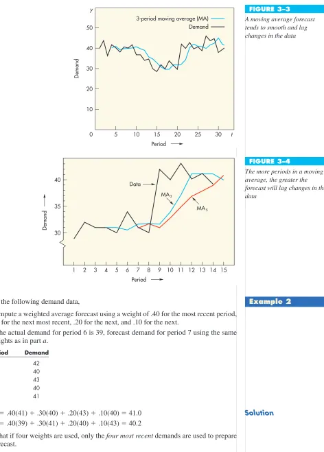
Figure 3–3 illustrates a three-period moving average forecast plotted against actual demand over 31 periods. Note how the moving average forecast lags the actual values and how smooth the forecasted values are compared with the actual values.
The moving average can incorporate as many data points as desired. In selecting the number of periods to include, the decision maker must take into account that the number of data points in the average determines its sensitivity to each new data point: The fewer the data points in an average, the more sensitive (responsive) the average tends to be. (See Figure 3–4.) If responsiveness is important, a moving average with relatively few data points should be used. This will permit quick adjustment to, say, a step change in the data, but it will also cause the forecast to be somewhat responsive even to random variations. Conversely, moving averages based on more data points will smooth more but be less re-sponsive to “real” changes. Hence, the decision maker must weigh the cost of responding more slowly to changes in the data against the cost of responding to what might simply be random variations. A review of forecast errors can help in this decision.
The advantages of a moving average forecast are that it is easy to compute and easy to understand. A possible disadvantage is that all values in the average are weighted equally. For instance, in a 10-period moving average, each value has a weight of 1/10. Hence, the oldest value has the same weight as the most recent value. If a change occurs in the series, a moving average forecast can be slow to react, especially if there are a large number of values in the average. Decreasing the number of values in the average increases the weight of more recent values, but it does so at the expense of losing potential information from less recent values.
Weighted Moving Average. A weighted average is similar to a moving average, ex-cept that it assigns more weight to the most recent values in a time series. For instance, the most recent value might be assigned a weight of .40, the next most recent value a weight of .30, the next after that a weight of .20, and the next after that a weight of .10. Note that the weights sum to 1.00, and that the heaviest weights are assigned to the most recent values.
F7
404139
3 40.00
F6
434041
3 41.33
Solution
Given the following demand data,
a. Compute a weighted average forecast using a weight of .40 for the most recent period, .30 for the next most recent, .20 for the next, and .10 for the next.
b. If the actual demand for period 6 is 39, forecast demand for period 7 using the same weights as in part a.
Period Demand
1 42
2 40
3 43
4 40
5 41
a. F6.40(41) .30(40) .20(43) .10(40) 41.0 b. F7.40(39) .30(41) .20(40) .10(43) 40.2
Note that if four weights are used, only the four most recent demands are used to prepare the forecast.
Period 6
4 5
3 2
1 7 8 9 10 11 12 13 14 15
40
35
30
Demand
Data
MA3
MA5
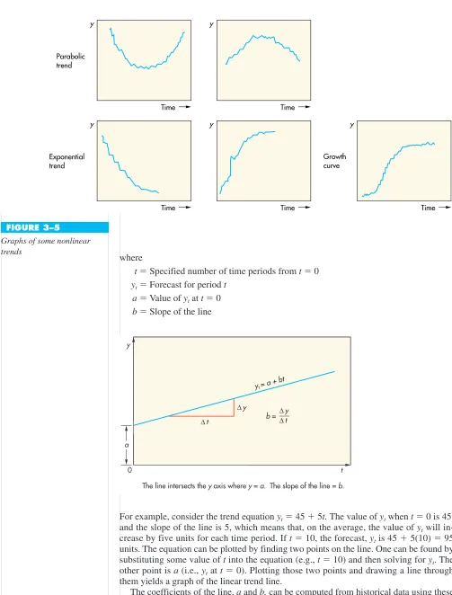
FIGURE 3–4
The more periods in a moving average, the greater the forecast will lag changes in the data
y
50
40
30
20
10
5
Period
10 15 20 25 30
0 t
Demand
3-period moving average (MA) Demand
FIGURE 3–3
A moving average forecast tends to smooth and lag changes in the data
Example 2
The advantage of a weighted average over a simple moving average is that the weighted average is more reflective of the most recent occurrences. However, the choice of weights is somewhat arbitrary and generally involves the use of trial and error to find a suitable weighting scheme.
Exponential Smoothing. Exponential smoothing is a sophisticated weighted
averag-ing method that is still relatively easy to use and understand. Each new forecast is based on the previous forecast plus a percentage of the difference between that forecast and the actual value of the series at that point. That is:
Next forecast Previous forecast (Actual Previous forecast)
where (Actual Previous forecast) represents the forecast error and is a percentage of the error. More concisely,
FtFt1 (At1Ft1) (3–2a)
where
FtForecast for period t
Ft1Forecast for the previous period Smoothing constant
At1Actual demand or sales for the previous period
The smoothing constant represents a percentage of the forecast error. Each new forecast is equal to the previous forecast plus a percentage of the previous error. For example, sup-pose the previous forecast was 42 units, actual demand was 40 units, and .10. The new forecast would be computed as follows:
Ft42 .10(40 42) 41.8
Then, if the actual demand turns out to be 43, the next forecast would be: Ft41.8 .10(43 41.8) 41.92
An alternate form of formula 3–2a reveals the weighting of the previous forecast and the latest actual demand:
Ft(1 )Ft1 At1 (3–2b)
For example, if .10, this would be Ft.90Ft1.10 At1
The quickness of forecast adjustment to error is determined by the smoothing constant, . The closer its value is to zero, the slower the forecast will be to adjust to forecast errors (i.e., the greater the smoothing). Conversely, the closer the value of is to 1.00, the greater the responsiveness and the less the smoothing. This is illustrated in Example 3.
The following table illustrates two series of forecasts for a data set, and the resulting (Actual Forecast) Error, for each period. One forecast uses .10 and one uses
.40. The following figure plots the actual data and both sets of forecasts.
.10 .40
Actual
Period (t) Demand Forecast Error Forecast Error
1 42 — — — —
2 40 42 2 42 2
3 43 41.8 1.2 41.2 1.8
4 40 41.92 1.92 41.92 1.92
5 41 41.73 0.73 41.15 0.15
exponential smoothing Weighted averaging method based on previous forecast plus a percentage of the forecast error.
6 39 41.66 2.66 41.09 2.09
7 46 41.39 4.61 40.25 5.75
8 44 41.85 2.15 42.55 1.45
9 45 42.07 2.93 43.13 1.87
10 38 42.35 4.35 43.88 5.88
11 40 41.92 1.92 41.53 1.53
12 41.73 40.92
Selecting a smoothing constant is basically a matter of judgment or trial and error, us-ing forecast errors to guide the decision. The goal is to select a smoothus-ing constant that balances the benefits of smoothing random variations with the benefits of responding to real changes if and when they occur. Commonly used values of range from .05 to .50. Low values of are used when the underlying average tends to be stable; higher values are used when the underlying average is susceptible to change.
Some computer packages include a feature that permits automatic modification of the smoothing constant if the forecast errors become unacceptably large.
Exponential smoothing is one of the most widely used techniques in forecasting, partly because of its ease of calculation, and partly because of the ease with which the weight-ing scheme can be altered—simply by changweight-ing the value of .
Note. A number of different approaches can be used to obtain a starting forecast, such as the average of the first several periods, a subjective estimate, or the first actual value as the forecast for period 2 (i.e., the naive approach). For simplicity, the naive approach is used in this book. In practice, using an average of, say, the first three values as a forecast for period 4 would provide a better starting forecast because that would tend to be more representative.
TECHNIQUES FOR TREND
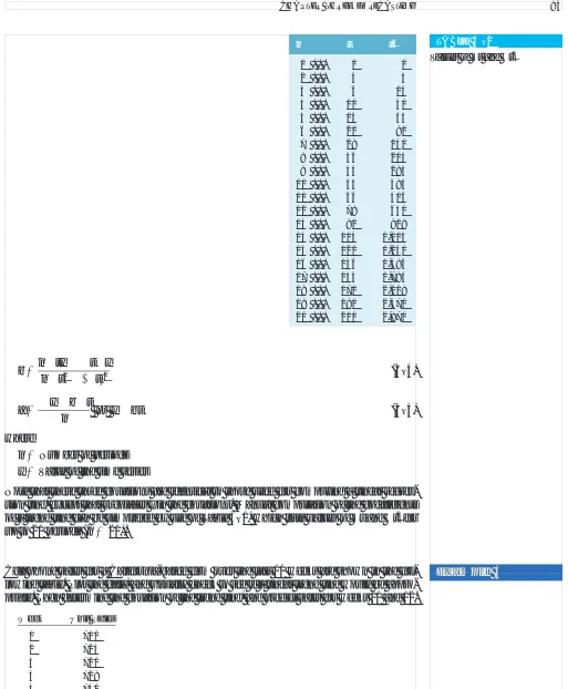
Analysis of trend involves developing an equation that will suitably describe trend (as-suming that trend is present in the data). The trend component may be linear, or it may not. Some commonly encountered nonlinear trend types are illustrated in Figure 3–5. A simple plot of the data can often reveal the existence and nature of a trend. The discussion here focuses exclusively on linear trends because these are fairly common.
There are two important techniques that can be used to develop forecasts when trend is present. One involves use of a trend equation; the other is an extension of exponential smoothing.
Trend Equation. A linear trend equation has the form
ytabt (3–3)
Period
Actual
α= .4
α= .1 45
40
Demand
2 4 6 8 10 12
0
linear trend equation yt abt , used to develop
where
tSpecified number of time periods from t0 ytForecast for period t
aValue of ytat t0
bSlope of the line
For example, consider the trend equation yt45 5t. The value of ytwhen t0 is 45, and the slope of the line is 5, which means that, on the average, the value of ytwill in-crease by five units for each time period. If t10, the forecast, ytis 45 5(10) 95 units. The equation can be plotted by finding two points on the line. One can be found by substituting some value of t into the equation (e.g., t10) and then solving for yt. The other point is a (i.e., ytat t0). Plotting those two points and drawing a line through them yields a graph of the linear trend line.
The coefficients of the line, a and b, can be computed from historical data using these two equations:
y
t 0
a
t
y
t y b=
yt=a+ bt
The line intersects theyaxis wherey=a. The slope of the line =b.
∆
∆
∆ ∆
Time y
Time y
Time y
Time y
Time y
Parabolic trend
Exponential trend
Growth curve
(3–4)
(3–5)
where
nNumber of periods yValue of the time series
Note that these three equations are identical to those used for computing a linear regres-sion line, except that t replaces x in the equations. Manual computation of the coefficients of a trend line can be simplified by use of Table 3–1, which lists values of t and t2for up to 20 periods (n20).
Cell phone sales for a California-based firm over the last 10 weeks are shown in the fol-lowing table. Plot the data, and visually check to see if a linear trend line would be appro-priate. Then determine the equation of the trend line, and predict sales for weeks 11 and 12.
Week Unit Sales
1 700
2 724
3 720
4 728
5 740
6 742
7 758
8 750
9 770
10 775
a
ybt n or y-
b t -bn
tytyn
t2t2Example 4
n t t2
1 . . . 1 1
2 . . . 3 5
3 . . . 6 14
4 . . . 10 30
5 . . . 15 55
6 . . . 21 91
7 . . . 28 140
8 . . . 36 204
9 . . . 45 285
10 . . . 55 385
11 . . . 66 506
12 . . . 78 650
13 . . . 91 819
14 . . . 105 1,015 15 . . . 120 1,240 16 . . . 136 1,496 17 . . . 153 1,785 18 . . . 171 2,109 19 . . . 190 2,470 20 . . . 210 2,870
a. A plot suggests that a linear trend line would be appropriate:
b. Week
(t ) y ty
1 700 700
2 724 1,448
3 720 2,160
4 728 2,912
5 740 3,700
6 742 4,452
7 758 5,306
8 750 6,000
9 770 6,930
10 775 7,750
7,407 41,358
From Table 3–1, for n10, t55 and t2 385. Using Formulas 3–4 and 3–5, you can compute the coefficients of the trend line:
Thus, the trend line is yt699.40 7.51t, where t0 for period 0.
c. Substituting values of t into this equation, the forecasts for the next two periods (i.e., t11 and t12) are:
y11699.40 7.51(11) 782.01 y12699.40 7.51(12) 789.52
d. For purposes of illustration, the original data, the trend line, and the two projections (forecasts) are shown on the following graph:
a7,4077.5155
10 699.40
b1041,358557,407 103855555
6,195 825 7.51
Week
2 4 6 8 10 12
1 3 5 7 9 11
780
760
740
720
700
Sales
TREND-ADJUSTED EXPONENTIAL SMOOTHING
A variation of simple exponential smoothing can be used when a time series exhibits trend. It is called trend-adjusted exponential smoothing or, sometimes, double smooth-ing, to differentiate it from simple exponential smoothsmooth-ing, which is appropriate only when data vary around an average or have step or gradual changes. If a series exhibits trend, and simple smoothing is used on it, the forecasts will all lag the trend: if the data are increas-ing, each forecast will be too low; if decreasincreas-ing, each forecast will be too high. Again, plotting the data can indicate when trend-adjusted smoothing would be preferable to sim-ple smoothing.
The trend-adjusted forecast (TAF) is composed of two elements: a smoothed error and a trend factor.
TAFt1StTt (3–6)
where
StSmoothed forecast
TtCurrent trend estimate and
StTAFt (AtTAFt) (3–7)
TtTt1 (TAFtTAFt1Tt1)
where and are smoothing constants. In order to use this method, one must select val-ues of and (usually through trial and error) and make a starting forecast and an esti-mate of trend.
Using the cell phone data from the previous example (where it was concluded that the data exhibited a linear trend), use trend-adjusted exponential smoothing to prepare fore-casts for periods 5 through 11, with 1.4 and 2.3.
The initial estimate of trend is based on the net change of 28 for the three changes from period 1 to period 4, for an average of 9.30. The data and calculations are shown in
Week
2 4 6 8 10 12
1 3 5 7 9 11
800
780
760
740
720
700
Sales
Trend line Data
Forecasts
trend-adjusted exponential smoothing Variation of expo-nential smoothing used when a time series exhibits trend.
Example 5
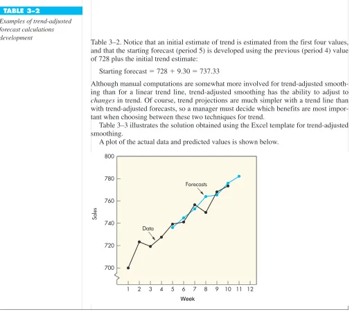
Table 3–2. Notice that an initial estimate of trend is estimated from the first four values, and that the starting forecast (period 5) is developed using the previous (period 4) value of 728 plus the initial trend estimate:
Starting forecast 728 9.30 737.33
Although manual computations are somewhat more involved for trend-adjusted smooth-ing than for a linear trend line, trend-adjusted smoothsmooth-ing has the ability to adjust to changes in trend. Of course, trend projections are much simpler with a trend line than with trend-adjusted forecasts, so a manager must decide which benefits are most impor-tant when choosing between these two techniques for trend.
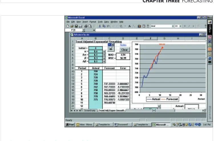
Table 3–3 illustrates the solution obtained using the Excel template for trend-adjusted smoothing.
A plot of the actual data and predicted values is shown below.
Week
2 4 6 8 10 12
1 3 5 7 9 11
800
780
760
740
720
700
Sales
Data
Forecasts
t At
(Period) (Actual)
1 700
Model 2 724
development 3 720
4 728
Ft TAFt (At TAFt) St Tt1 (TAFt TAFt1 Tt1) Tt
5 740 737.33 737.33 .4(740 737.33) 738.40 9.33 .3(0) 9.33
6 742 747.73 747.73 .4(742 747.73) 745.44 9.33 .3(747.73 737.33 9.33) 9.65 Model 7 758 755.09 755.09 .4(758755.09) 756.25 9.65 .3(755.09 747.739.65) 8.96 test 8 750 765.22 765.22 .4(750765.22) 759.13 8.96.3(765.22 755.098.96) 9.31 9 770 768.45 768.45 .4(770768.45) 769.07 9.31.3(768.45 765.229.31) 7.49 10 775 776.56 776.56 .4(775776.56) 775.94 7.49.3(776.56 768.457.49) 7.68
Forecast 11 783.61 [ 775.94 7.68]
Note: Some numbers don’t add exactly due to rounding. TABLE 3–2
Examples of trend-adjusted forecast calculations development
TECHNIQUES FOR SEASONALITY
Seasonal variations in time series data are regularly repeating upward or downward
movements in series values that can be tied to recurring events. Seasonality may refer to regular annual variations. Familiar examples of seasonality are weather variations (e.g., sales of winter and summer sports equipment) and vacations or holidays (e.g., airline travel, greeting card sales, visitors at tourist and resort centers). The term seasonal varia-tion is also applied to daily, weekly, monthly, and other regularly recurring patterns in data. For example, rush hour traffic occurs twice a day—incoming in the morning and outgoing in the late afternoon. Theaters and restaurants often experience weekly demand patterns, with demand higher later in the week. Banks may experience daily seasonal vari-ations (heavier traffic during the noon hour and just before closing), weekly varivari-ations (heavier toward the end of the week), and monthly variations (heaviest around the begin-ning of the month because of social security, payroll, and welfare checks being cashed or deposited). Mail volume; sales of toys, beer, automobiles, and turkeys; highway usage; hotel registrations; and gardening also exhibit seasonal variations.
Seasonality in a time series is expressed in terms of the amount that actual values de-viate from the average value of a series. If the series tends to vary around an average value, then seasonality is expressed in terms of that average (or a moving average); if trend is present, seasonality is expressed in terms of the trend value.
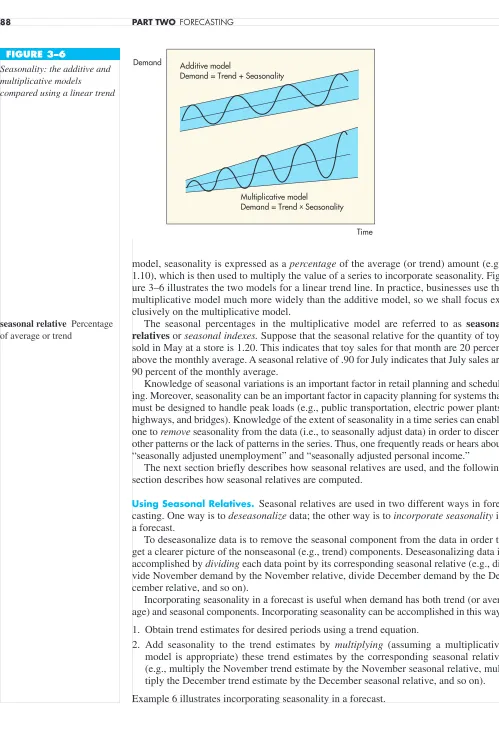
There are two different models of seasonality: additive and multiplicative. In the addi-tive model, seasonality is expressed as a quantity (e.g., 20 units), which is added or sub-tracted from the series average in order to incorporate seasonality. In the multiplicative
TABLE 3–3
Using the Excel template for trend-adjusted smoothing
Demand for products such as lawnmowers and snow throwers is subject to large seasonal fluctuations. Toro matches these fluctuations by reallocating its manufacturing capacity between products. seasonal variations Regularly repeating movements in series values that can be tied to recur-ring events.
model, seasonality is expressed as a percentage of the average (or trend) amount (e.g., 1.10), which is then used to multiply the value of a series to incorporate seasonality. Fig-ure 3–6 illustrates the two models for a linear trend line. In practice, businesses use the multiplicative model much more widely than the additive model, so we shall focus ex-clusively on the multiplicative model.
The seasonal percentages in the multiplicative model are referred to as seasonal
relatives or seasonal indexes. Suppose that the seasonal relative for the quantity of toys
sold in May at a store is 1.20. This indicates that toy sales for that month are 20 percent above the monthly average. A seasonal relative of .90 for July indicates that July sales are 90 percent of the monthly average.
Knowledge of seasonal variations is an important factor in retail planning and schedul-ing. Moreover, seasonality can be an important factor in capacity planning for systems that must be designed to handle peak loads (e.g., public transportation, electric power plants, highways, and bridges). Knowledge of the extent of seasonality in a time series can enable one to remove seasonality from the data (i.e., to seasonally adjust data) in order to discern other patterns or the lack of patterns in the series. Thus, one frequently reads or hears about “seasonally adjusted unemployment” and “seasonally adjusted personal income.”
The next section briefly describes how seasonal relatives are used, and the following section describes how seasonal relatives are computed.
Using Seasonal Relatives. Seasonal relatives are used in two different ways in fore-casting. One way is to deseasonalize data; the other way is to incorporate seasonality in a forecast.
To deseasonalize data is to remove the seasonal component from the data in order to get a clearer picture of the nonseasonal (e.g., trend) components. Deseasonalizing data is accomplished by dividing each data point by its corresponding seasonal relative (e.g., di-vide November demand by the November relative, didi-vide December demand by the De-cember relative, and so on).
Incorporating seasonality in a forecast is useful when demand has both trend (or aver-age) and seasonal components. Incorporating seasonality can be accomplished in this way: 1. Obtain trend estimates for desired periods using a trend equation.
2. Add seasonality to the trend estimates by multiplying (assuming a multiplicative model is appropriate) these trend estimates by the corresponding seasonal relative (e.g., multiply the November trend estimate by the November seasonal relative, mul-tiply the December trend estimate by the December seasonal relative, and so on). Example 6 illustrates incorporating seasonality in a forecast.
seasonal relative Percentage of average or trend
Time Demand
Multiplicative model
Demand = Trend x Seasonality Additive model
Demand = Trend + Seasonality FIGURE 3–6
A furniture manufacturer wants to predict quarterly demand for a certain loveseat for pe-riods 15 and 16, which happen to be the second and third quarters of a particular year. The series consists of both trend and seasonality. The trend portion of demand is projected us-ing the equation yt124 7.5t. Quarter relatives are Q11.20, Q21.10, Q30.75, and Q40.95. Use this information to predict demand for periods 15 and 16.
The trend values at t 15 and t16 are: y15124 7.5(15) 236.5
y16124 7.5(16) 244.0
Multiplying the trend value by the appropriate quarter relative yields a forecast that in-cludes both trend and seasonality. Given that t15 is a second quarter and t16 is a third quarter, the forecasts are:
Period 15: 236.5(1.10) 260.15 Period 16: 244.0(0.75) 183.00
Computing Seasonal Relatives. A commonly used method for representing the trend portion of a time series involves a centered moving average. Computations and the re-sulting values are the same as those for a moving average forecast. However, the values are not projected as in a forecast; instead, they are positioned in the middle of the periods used to compute the moving average. The implication is that the average is most repre-sentative of that point in the series. For example, assume the following time series data:
Three-Period Period Demand Centered Average
1 40
2 46 42.67
3 42
The three-period average is 42.67. As a centered average, it is positioned at period 2; the average is most representative of the series at that point.
The ratio of demand at period 2 to this centered average at period 2 is an estimate of the seasonal relative at that point. Because the ratio is 46/42.67 1.08, the series is about 8 percent above average at that point. To achieve a reasonable estimate of seasonality for any season (e.g., Friday attendance at a theater), it is usually necessary to compute sea-sonal ratios for a number of seasons and then average these ratios. In the case of theater attendance, average the ratios of five or six Fridays for the Friday relative, average five or six Saturdays for the Saturday relative, and so on.
The manager of a parking lot has computed daily relatives for the number of cars per day in the lot. The computations are repeated here (about three weeks are shown for illustra-tion). A seven-period centered moving average is used because there are seven days (sea-sons) per week.
Day Volume Moving Total Centered MA7 Volume/MA
Tues 67
Wed 75
Thur 82
Fri 98 71.86 98/71.86 1.36 (Friday)
Sat 90 70.86 90/70.86 1.27
Sun 36 70.57 36/70.57 0.51
Mon 55 503 ÷ 7 71.00 55/71.00 0.77
Tues 60 496 ÷ 7 71.14 60/71.14 0.84 (Tuesday)
Average40463 4242.67
Example 6
Solution
centered moving average A moving average positioned at the center of the data that were used to compute it.
Wed 73 494 etc. 70.57 73/70.57 1.03
Thur 85 497 71.14 85/71.14 1.19
Fri 99 498 70.71 99/70.71 1.40 (Friday)
Sat 86 494 71.29 86/71.29 1.21
Sun 40 498 71.71 40/71.71 0.56
Mon 52 495 72.00 52/72.00 0.72
Tues 64 499 71.57 64/71.57 0.89 (Tuesday)
Wed 76 502 71.86 76/71.86 1.06
Thur 87 504 72.43 87/72.43 1.20
Fri 96 501 72.14 96/72.14 1.33 (Friday)
Sat 88 503
Sun 44 507
Mon 50 505
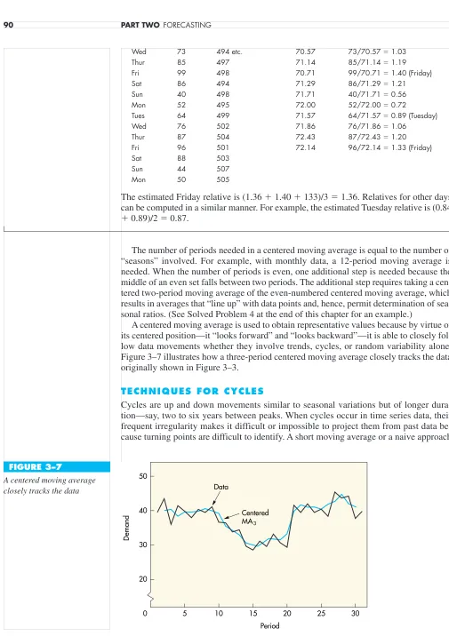
The estimated Friday relative is (1.36 1.40 133)/3 1.36. Relatives for other days can be computed in a similar manner. For example, the estimated Tuesday relative is (0.84 0.89)/2 0.87.
The number of periods needed in a centered moving average is equal to the number of “seasons” involved. For example, with monthly data, a 12-period moving average is needed. When the number of periods is even, one additional step is needed because the middle of an even set falls between two periods. The additional step requires taking a cen-tered two-period moving average of the even-numbered cencen-tered moving average, which results in averages that “line up” with data points and, hence, permit determination of sea-sonal ratios. (See Solved Problem 4 at the end of this chapter for an example.)
A centered moving average is used to obtain representative values because by virtue of its centered position—it “looks forward” and “looks backward”—it is able to closely fol-low data movements whether they involve trends, cycles, or random variability alone. Figure 3–7 illustrates how a three-period centered moving average closely tracks the data originally shown in Figure 3–3.
TECHNIQUES FOR CYCLES
Cycles are up and down movements similar to seasonal variations but of longer dura-tion—say, two to six years between peaks. When cycles occur in time series data, their frequent irregularity makes it difficult or impossible to project them from past data be-cause turning points are difficult to identify. A short moving average or a naive approach
50
40
30
20
5
Period
10 15 20 25 30
0
Demand
Centered MA3
Data
FIGURE 3–7
may be of some value, although both will produce forecasts that lag cyclical movements by one or several periods.
The most commonly used approach is explanatory: Search for another variable that re-lates to, and leads, the variable of interest. For example, the number of housing starts (i.e., permits to build houses) in a given month often is an indicator of demand a few months later for products and services directly tied to construction of new homes (landscaping; sales of washers and dryers, carpeting, and furniture; new demands for shopping, trans-portation, schools). Thus, if an organization is able to establish a high correlation with such a leading variable (i.e., changes in the variable precede changes in the variable of in-terest), it can develop an equation that describes the relationship, enabling forecasts to be made. It is important that a persistent relationship exists between the two variables. More-over, the higher the correlation, the better the chances that the forecast will be on target.
Associative Forecasting Techniques
Associative techniques rely on identification of related variables that can be used to pre-dict values of the variable of interest. For example, sales of beef may be related to the price per pound charged for beef and the prices of substitutes such as chicken, pork, and lamb; real estate prices are usually related to property location; and crop yields are related to soil conditions and the amounts and timing of water and fertilizer applications.
The essence of associative techniques is the development of an equation that summa-rizes the effects of predictor variables. The primary method of analysis is known as
regression. A brief overview of regression should suffice to place this approach into
per-spective relative to the other forecasting approaches described in this chapter.
SIMPLE LINEAR REGRESSION
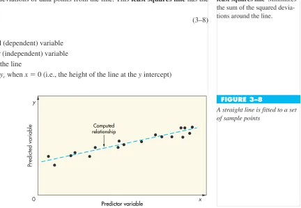
The simplest and most widely used form of regression involves a linear relationship be-tween two variables. A plot of the values might appear like that in Figure 3–8. The object in linear regression is to obtain an equation of a straight line that minimizes the sum of squared vertical deviations of data points from the line. This least squares line has the equation
ycabx (3–8)
where
ycPredicted (dependent) variable
xPredictor (independent) variable bSlope of the line
aValue of ycwhen x0 (i.e., the height of the line at the y intercept)
y
Predictor variable x
0
Predicted variable
Computed relationship
FIGURE 3–8
A straight line is fitted to a set of sample points
predictor variables Variables that can be used to predict val-ues of the variable of interest.
regression Technique for fit-ting a line to a set of points.
(Note: It is conventional to represent values of the predicted variable on the y axis and values of the predictor variable on the x axis.) Figure 3–9 is a graph of a linear regression line.
The coefficients a and b of the line are computed using these two equations:
(3–9)
(3–10)
where
nNumber of paired observations
Healthy Hamburgers has a chain of 12 stores in northern Illinois. Sales figures and prof-its for the stores are given in the following table. Obtain a regression line for the data, and predict profit for a store assuming sales of $10 million.
Sales, x Profits, y (in millions of dollars)
$ 7 $0.15
2 0.10
6 0.13
4 0.15
14 0.25
15 0.27
16 0.24
12 0.20
14 0.27
20 0.44
15 0.34
7 0.17
First, plot the data and decide if a linear model is reasonable (i.e., do the points seem to scatter around a straight line? Figure 3–10 suggests they do). Next, compute the quanti-ties x,y,xy and x2). Calculations are shown for these quantities in Table 3–4. One additional calculation, y2), is included for later use.
a
ybxn or y
-bx
bn
xyxy nx2x2Example 8
Solution
y
x 0
a
x
y
x y b=
yc=a+ bx
The line intersects theyaxis wherey=a. The slope of the line =b.
∆
∆
∆ ∆
FIGURE 3–9
Substituting into the equation, you find:
Thus, the regression equation is: yc0.0506 0.01593x. For sales of x10 (i.e., $10 million), estimated profit is: yc0.0506 0.01593(10) 0.2099, or $209,900. (It may appear strange that substituting x 0 into the equation produces a predicted profit of $50,600 because it seems to suggest that amount of profit will occur with no sales. How-ever, the value of x 0 is outside the range of observed values. The regression line should be used only for the range of values from which it was developed; the relationship may be nonlinear outside that range. The purpose of the a value is simply to establish the height of the line where it crosses the y axis.)
One application of regression in forecasting relates to the use of indicators. These are un-controllable variables that tend to lead or precede changes in a variable of interest. For ex-ample, changes in the Federal Reserve Board’s discount rate may influence certain business activities. Similarly, an increase in energy costs can lead to price increases for a wide range of products and services. Careful identification and analysis of indicators may
a
ybxn
2.710.01593132
12 0.0506
bn
xyxy nx2x21235.291322.271
121,796132132 0.01593 50
40
30
20
10
0
2 4 6 8 10 12 14 16 18 20
Sales ($ millions)
Profits ($ ten thousands)
FIGURE 3–10 A linear model seems reasonable
x y xy x2 y2
7 0.15 1.05 49 0.0225
2 0.10 0.20 4 0.0100
6 0.13 0.78 36 0.0169
4 0.15 0.60 16 0.0225
14 0.25 3.50 196 0.0625
15 0.27 4.05 225 0.0729
16 0.24 3.84 256 0.0576
12 0.20 2.40 144 0.0400
14 0.27 3.78 196 0.0729
20 0.44 8.80 400 0.1936
15 0.34 5.10 225 0.1156
7 0.17 1.19 49 0.0289
132 2.71 35.29 1,796 0.7159
TABLE 3–4
yield insight into possible future demand in some situations. There are numerous pub-lished indexes and websites from which to choose.1These include:
Net change in inventories on hand and on order. Interest rates for commercial loans.
Industrial output.
Consumer price index (CPI). The wholesale price index. Stock market prices.
Other potential indicators are population shifts, local political climates, and activities of other firms (e.g., the opening of a shopping center may result in increased sales for nearby businesses). Three conditions are required for an indicator to be valid:
1. The relationship between movements of an indicator and movements of the variable should have a logical explanation.
2. Movements of the indicator must precede movements of the dependent variable by enough time so that the forecast isn’t outdated before it can be acted upon.
3. A fairly high correlation should exist between the two variables.
Correlation measures the strength and direction of relationship between two variables.
Correlation can range from 1.00 to 1.00. A correlation of 1.00 indicates that changes in one variable are always matched by changes in the other; a correlation of 1.00 indicates that increases in one variable are matched by decreases in the other; and a correlation close to zero indicates little linear relationship between two variables. The correlation between two variables can be computed using the equation
(3–11)
The square of the correlation coefficient, r2, provides a measure of the percentage of vari-ability in the values of y that is “explained” by the independent variable. The possible val-ues of r2range from 0 to 1.00. The closer r2 is to 1.00, the greater the percentage of explained variation. A high value of r2, say .80 or more, would indicate that the indepen-dent variable is a good predictor of values of the depenindepen-dent variable. A low value, say .25 or less, would indicate a poor predictor, and a value between .25 and .80 would indicate a moderate predictor.
COMMENTS ON THE USE OF LINEAR REGRESSION ANALYSIS
Use of simple regression analysis implies that certain assumptions have been satisfied. Basically, these are:
1. Variations around the line are random. If they are random, no patterns such as cycles or trends should be apparent when the line and data are plotted.
2. Deviations around the line should be normally distributed. A concentration of values close to the line with a small proportion of larger deviations supports the assumption of normality.
3. Predictions are being made only within the range of observed values.
If the assumptions are satisfied, regression analysis can be a powerful tool. To obtain the best results, observe the following:
1. Always plot the data to verify that a linear relationship is appropriate.
r n
xyxyn
x2x2ny2y21See, for example, The National Bureau of Economic Research, The Survey of Current Business, The
Monthly Labor Review, and Business Conditions Digest. correlation A measure of
2. The data may be time-dependent. Check this by plotting the dependent variable versus time; if patterns appear, use analysis of time series instead of regression, or use time as an independent variable as part of a multiple regression analysis.
3. A small correlation may imply that other variables are important. In addition, note these weaknesses of regression:
1. Simple linear regression applies only to linear relationships with one independent variable.
2. One needs a considerable amount of data to establish the relationship—in practice, 20 or more observations.
3. All observations are weighted equally.
Sales of 19-inch color television sets and three-month lagged unemployment are shown in the following table. Determine if unemployment levels can be used to predict demand for 19-inch color TVs and, if so, derive a predictive equation.
Period . . . 1 2 3 4 5 6 7 8 9 10 11
Units sold . . . 20 41 17 35 25 31 38 50 15 19 14 Unemployment %
(three-month lag) . . 7.2 4.0 7.3 5.5 6.8 6.0 5.4 3.6 8.4 7.0 9.0
1. Plot the data to see if a linear model seems reasonable. In this case, a linear model seems appropriate for the range of the data.
2. Compute the correlation coefficient to confirm that it is not close to zero.
x y xy x2 y2
7.2 20 144.0 51.8 400
4.0 41 164.0 16.0 1,681
7.3 17 124.1 53.3 289
5.5 35 192.5 30.3 1,225
6.8 25 170.0 46.2 625
6.0 31 186.0 36.0 961
5.4 38 205.2 29.2 1,444
3.6 50 180.0 13.0 2,500
8.4 15 126.0 70.6 225
7.0 19 133.0 49.0 361
9.0 14 126.0 81.0 196
70.2 305 1,750.8 476.4 9,907
50
40
30
20
10
0
2 4 6 8 10
Level of unemployment (%),x
Units sold,
y
Example 9
This is a fairly high negative correlation. 3. Compute the regression line:
Note that the equation pertains only to unemployment levels in the range 3.6 to 9.0, be-cause sample observations covered only that range.
CURVILINEAR AND MULTIPLE REGRESSION ANALYSIS Simple linear regression may prove inadequate to handle certain problems because a lin-ear model is inappropriate or because more than one predictor variable is involved. When nonlinear relationships are present, you should employ curvilinear regression; models that involve more than one predictor require the use of multiple regression analysis. While these analyses are beyond the scope of this text, you should be aware that they are often used. The computations lend themselves more to computers than to hand calculation. Multiple regression forecasting substantially increases data requirements. In each case, it is necessary to weigh the additional cost and effort against potential improvements in ac-curacy of predictions.
Accuracy and Control of Forecasts
Accuracy and control of forecasts is a vital aspect of forecasting. The complex nature of most real-world variables makes it almost impossible to correctly predict future values of those variables on a regular basis. Consequently, it is im