The Tandem Counting Bloom Filter - It Takes Two Counters to Tango

The Tandem Counting Bloom Filter - It Takes

Two Counters to Tango

Pedro Reviriego and Ori Rottenstreich

Abstract—Set representation is a crucial functionality in various areas such as networking and databases. In many applications, memory and time constraints allow only an approximate represen-tation where errors can appear for some queried elements. The Variable-Increment Counting Bloom Filter (VI-CBF) is a popular data structure for the representation of dynamically-changing sets, achieving a good tradeoff between memory efficiency and queries accuracy. For some applications, the required accuracy is higher than that enabled by the VI-CBF. In this paper, we present the Tandem Counting Bloom Filter (T-CBF), a new data structure that relies on the interaction among counters to describe sets with higher accuracy. We analyze its performance and show that by a joint consideration of counters, the T-CBF always performs better than the VI-CBF and it can for some configurations reduce its false positive probability by an order of magnitude. The overhead of such an approach is expressed upon an element insertion or query as read or write operations to a pair of counters rather than a single counter in each hash location. The operations themselves also require considering a larger number of scenarios.

I. INTRODUCTION

A. Background

Set representation is a required technique in many applications such as caching, routing and packet classification. While the represented set S is often assumed to be finite, it can be taken from a finite or an infinite universe U. There are two kinds of errors in membership queries: a false positive (when an element

x /∈S is reported as a member ofS) and a false negative (when an element x ∈ S is reported as a non member of S). The Bloom filter [1], [2] is a popular data structure used for that manner, supporting membership queries. The Bloom filter is probabilistic in a sense that it can incorrectly answer queries for some elements. The Bloom filter encounters false positives and has no false negatives. The probability for an error (ratio of non-member elements reported as non-members) decreases when more memory is allocated for the data structure and increases when a larger set S is represented. The Bloom filter stores an array of bits, where a set of hash functions is used to map elements to locations in the bit array. With initial values of zero bits, the elements of S are first mapped to the filter, setting all bits pointed by the hash functions. Upon a query, the bits pointed by the queried element are examined and a positive answer is returned only when the bits are all set.

The Counting Bloom filter (CBF) [3] generalizes the basic Bloom filter with the support of element removals (deletions). This is a crucial functionality when the represented set is

P. Reviriego is with Universidad Carlos III de Madrid, Avda de la Universidad 30, Leganes, Madrid, Spain. email: [email protected].

O. Rottenstreich is with the Department of Computer Science and the Viterbi Department of Electrical Engineering, Technion, Israel. email: [email protected].

dynamic and its size can change over time. The CBF maintains an array of counters instead of an array of bits as in the Bloom filter. Upon an element insertion, counters mapped by the hash function are increased by one. Upon a query, the same counters are examined. In case they are all non-zero a positive answer is returned for the query. In the CBF, besides the fact whether the counter is positive or not, the exact value of the counter is not taken into account during the query process.

The Variable-Increment Counting Bloom filter (VI-CBF) [4] improves the error-memory tradeoff of the CBF by considering the exact counter values upon a query. It relies on variable increments such that in an element insertion, counters are not increased by a fixed value but by values, selected by an additional set of hash functions, among a small set of variable increments. Then, upon a query, it is checked whether a given counter value can be comprised of the corresponding variable increment of the queried element. If this is not the case for one of the examined counters, membership can be eliminated.

The selection of the set of possible variable increments has a large impact on the achieved false positive rate. A simple selection of such a set is the rangeDL={L, . . . ,2L−1}. Notice

that for such a set, the sum is comprised of a single element only if the sum is in the range {L, . . . ,2L−1}. In such a case, it is also clear which increment was used. Likewise, if the sumc

is in {2L, . . . ,3L−1} then necessarily it is of two elements and the sum is not comprised of values larger thanc−L. This enables examining the membership through simple operations. Other selections of the set of increments have been suggested but have not been fully analyzed. Unlike the selection of DL

as the set, their implementation requires keeping an additional lookup table in memory. Also, note that with the set of variable increments of the VI-CBF as D =DL the counter values are restricted and never observe the values1, . . . , L−1. Along the paper while referring the VI-CBF, we assume that the set of variable increments is of the formD=DL.

As a common methodology for the Bloom filter, the CBF and the VI-CBF, a membership query is answered based on examining multiple hash locations with a single bit or counter. If based on any of them, we can deduce that membership has not occurred, a negative answer is given to the query. We refer to each such case as anelimination of the membership. Otherwise, namely when membership elimination cannot be deduced based on any of the hash locations with the particular examination of the scheme, a positive answer is given to the query.

any information to maintain more details regarding an element mapped to the other counter in the pair. While still available, such information can be further examined upon a membership query. Note that to identify a case where a counter holds information of element of the other counter in the pair, we should represent that in unique values. Accordingly, we also rely on variable increments since with fixed increments of one, a counter can possibly have all values. On the contrary, a set of variable increments D can imply a restricted set of possible counter values.

B. Motivation for Even Lower False Positive Probability

In the design of a system involving a Bloom filter or its variants, the system designer has to determine what should be the typical performance of the data structure expressed as its false positive probability. A restriction on this probability implies a lower bound on the required memory. Of course, there are no fixed globally desired values and each application with its properties implies various requirements. A recent study [5] shed light on that question. It examines the relative costs of the two possible errors in answering membership queries: a false positive and a false negative. This study focused on the case that both costs are finite. It shows that for the Bloom filter in order to be useful, its false positive probability must be below a bound implied by the data structure parameters and the ratios of the two costs. Assume a Bloom filter of a false positive probability pand that the cost of a false negative cost equals α times the cost of a false positive. Consider an element xwith a priori probabilityP r(x∈S)to belong to the represented set. This is the membership probability regardless of any information derived from the data structure. For instance, the probability equals for all elements |S|/|U| when a set S

is selected uniformly among a finite universe U. It is shown that the data structure is useless in serving such an element x

for a false positive probability p > ₁α₋·P r_{P r}(₍x_x∈_∈S_S)₎, namely when

P r(x ∈ S) < _p+p_α. Clearly, for a large universe, there are necessarily elements with relatively small a priori membership probabilities, implying a strict low upper bound on the false positive probability of the Bloom filter to be useful for keeping such elements among the represented set.

C. Network applications of Bloom filters

Bloom filters are widely used in many Networking appli-cations [6]. For example, they are used for packet inspection, spam filtering, caching systems and other security related tasks [7]. Typically along such applications Bloom filters are useful to speed up packet processing by performing an initial check through performing a query to the filter so that on a negative answer (that is necessarily correct due to the avoidance of false negatives in the filter) no further action is needed. On the contrary, if the answer is positive, additional processing of the packet is done according to the particular application. This is beneficial when the cost of querying the filter is much lower than that of processing the packet.

Consider for instance a distributed cache application where a local cache miss can be solved in one of several caches located in multiple network locations in a distributed manner [3].

A participant maintains Bloom filters to summarize the cache content of each of the other nodes. Upon a miss, it queries each of the filters and then access only those caches that correspond to filters with a positive answer. There is clearly no point in accessing caches with a negative indication since they do not have the element. (To allow dynamic changes in the filter content through support of deletions, often a Counting Bloom filter is used for this application.) Since the filters are maintained locally, accessing them is much cheaper than sending an access request to one of the other caches.

This is also the case, in some Longest Prefix Match (LPM) algorithms that perform a series of table lookups to find the best matching prefix. Existing prefixes in the classification table are organized in groups based on their length, with a Bloom filter associated with each group [8]. Given packet address, a query is performed in all filters. Only for those prefix lengths to which a positive answer is returned, it is required to check that a real match with a prefix of such length exists and no false positives have occurred. The longest found match determines the classification. Using Bloom filters was shown to reduce classification time upon considering all prefixes for each packet. The same approach has been used for the more general problem of packet classification where typically some fields of the header are matched against the rules stored on a table that can include wildcard bits or be based on multiple header fields. This classification can be decomposed also as a sequence of exact match lookups for which filtering can be beneficial [9].

The in-packet Bloom filter [10] allows a forwarding mech-anism developed for information centric networking, through encoding multicast trees in the packet header in a stateless manner. The filter effectively represents a set of nodes or link IDs along an expected path. While paths are often short, a node that receives a packet examines the filter and forwards it on its outgoing links that yield a positive membership indication.

Bloom filters are also useful for set synchronization, shar-ing information with potential overlap between multiple hosts through minimizing the amount of communication [11], [12], [13]. This can be a common practice in networks such as for exchanging missing block parts in a distributed file system or to share policy rules among switches in SDN networks.

Bloom filters have also been used to identify specific flows on the traffic [14], [15]. In this case, the identifier of a flow is the 5-tuple formed by source and destination IP addresses and transport ports and the protocol field. This requires more than 100 bits in IPv4 and close to 300 bits in IPv6. Therefore, a filtering using a smaller number of bits can be helpful to reduce memory bandwidth and power consumption.

In most of the applications discussed, the set represented by the filter changes over time. For example, in a routing table, routes are added and deleted and in a flow monitoring application flows start and end. Although the number and rate of the set changes is application specific, there is a need to support addition and removals and thus filters that support those operations.

II. BACKGROUND- THEVARIABLE-INCREMENTCOUNTING

BLOOM FILTER

rep-resented as an array of counters as in the Counting Bloom filter (CBF). However, an element insertion or a deletion are not implemented simply by a fixed addition of a subtraction of one to selected counters. The VI-CBF makes use of a set of integer variable increments D = {v1, v2, ..., v`}. We focus on

a particular selection of this set D as DL = [L,2L−1] = {L, L+ 1, . . . ,2L−1}that simplifies the implementation of the filter. It uses two sets of khash functions. Each function in the first set of hash functionsH ={h1, . . . , hk}maps an element to

one of the counters. Likewise, each function in a second set of hash functionsG={g1, . . . , gk}associates a variable increment for the element in each of the counters.

We explain the insertion, deletion and membership query operation for some element x.

Insertion: Upon insertion, at each corresponding counter in the array with an indexhi(x), the counter is incremented by the element vgi(x) of the setD.

Deletion: Upon deletion, counter hi(x) is decremented by

vgi(x)∈D.

Membership Query:To check whether the element belongs to the represented set, the counters with indices hi(x) are examined. If for (at least) one of them, its value ci implies that the sum is not comprised of the corresponding variable increment

vgi(x)the membership query returns a negative answer. For the

particular set of variable incrementsD= [L,2L−1]a sumcican

be comprised ofvgi(x)only if(c−vgi(x)) = 0or(c−vgi(x))≥L.

If for all i ∈ [1, k] ci can be comprised of vgi(x), the query

returns a positive answer which might be a false positive. It was shown that for a given memory size and the same number of elements, the VI-CBF achieves an improved false positive probability than the CBF. Denote by Pi the probability to have

i elements in a counter following the insertion of n elements usingkhash functions to an array ofmcounters. A formula for the VI-CBF false positive probability was presented in [4].

Property 1. The false positive probability of the VI-CBF equals

(1−p/∈)k for

p∈/ =P0+

L−1 L ·P1+

(L−1)(L+ 1) 6L2 ·P2

=1− 1 m

nk

+L−1 L

_nk

1

₁

m

1− 1 m

nk−1

+(L−1)(L+ 1) 6L2

_nk

2

₁

m

2

1− 1 m

nk−2

.

Pseudocode for the insertion, removal and membership query operations of the VI-CBF can later be found in Alg. 1, Alg. 3 and Alg. 5, respectively.

III. THETANDEMCOUNTINGBLOOMFILTER(T-CBF)

A. Motivation and Concept

The main motivation of the proposed scheme is to achieve a lower false positive rate than that of the VI-CBF (for a given amount of allocated memory). To do so, two observations are the key. The first one is that in the VI-CBF a counter never observes the values 1,2, . . . , L−1. This means that we can potentially use those values to encode additional information. The second observation is that by design, the VI-CBF relatively often has counters with no elements mapped to them. Since the

VI-CBF relies on having counters with zero, one or two mapped elements and the number of elements in a counter follows a binomial distribution, the probability for zero mapped elements cannot be negligible. In addition to these two properties, we also take advantage of a typical implementation where memory is accessed in unit of memory words, such that each word includes multiple counters.

The strategy of the suggested data structure, named the Tandem Counting Bloom Filter (T-CBF), is togroup counters in pairs where each pair of counters belongs to the same memory word. For example, we can consider a 32-bit word that stores four countersC1, C2, C3, C4, each of eight bits (a typical counter size in a construction of the VI-CBF). In that case,C1, C2 can form a pair and C3, C4 another pair. Then, when inserting an element x that maps to C1, we potentially store information also in the other counter in the pair C2. This information can be used to derive a more accurate answer to a query for further decreasing the false positive probability. This can be done when no element is mapped toC2 as marked by unique values

1,2, . . . , L−1 ofC2. This is the basic idea behind the T-CBF. The construction and operation of the T-CBF are discussed in more detail in the rest of this section.

B. Notation and Basics

Before describing the T-CBF in more detail, we define the notation used along the paper. The data structure represents a finite setS⊆U, whereUcan be finite or infinite. Hash functions are used to map elements to counters, to select the corresponding variable increments as well as the possible additional variable increments used for adjacent counters.

• m- number of counters in the data structure

• n- number of elements in the set S

• k- number of hash functions (for each of the three types)

• fi,i∈[1, k] - hash functions for counter selection • gi,i∈[1, k]- hash functions for the selection of increment

for the counter pointed byfi

• hi,i∈[1, k]- hash functions for the selection of increment for the counter paired to that pointed by fi

We assume a first set of variable increments V = {v1, . . . , vL} = {L, L+ 1, . . . ,2L −1} with an increment given by vg_i(x) for an element x in the counter fi(x). An additional set of variable increments isW ={w1, . . . , wL−1}=

{1,2, . . . , L−1}with an adjacent increment given bywhi(x)for

an elementx, possibly used in the counter adjacent tofi(x).

We illustrate the suggested scheme by consideringktimes, a pair of counters. For an elementxand some hash function index

i∈[1, k], we denote byC1the counter pointed byfi(x)and by

C2 its adjacent counter. We also refer to their values asc1 and

c2, respectively.

1 0 0 0 1 1 0 0 1 0

+1 +1 +1 +1

>0? >0?

x y

z

(a) CBF

6 0 0 0 5 7 0 0 4 0

+6 +5 +7 +4

6? 7?

x y

z

(b) VI-CBF

6 3 0 0 5 7 0 0 4 1

+6 +5 +7 +4

6? 7?

+3 +1

2?

x y

z

(c) T-CBF

Fig. 1. Illustration of the suggested T-CBF (in (c)) in comparison with the CBF (in (a)) and the VI-CBF (in (b)). Counters are organized in pairs. For each pointed counter, additional hash functions might be used to update / examine value of the adjacent counter based on its availability. Additional adjacent (used) hash functions appear in dotted arrows. The adjacent hash functions make use of a dedicated set of variable increments.

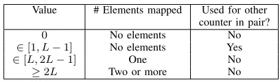
TABLE I

MEANING OF THE DIFFERENT COUNTER VALUES

Value # Elements mapped Used for other counter in pair?

0 No elements No

∈[1, L−1] No elements Yes ∈[L,2L−1] One No

≥2L Two or more No

is examined whether counter values can be comprised of some variable increment. In the T-CBF, as illustrated in (c), counters are organized in pairs and variable increments are again in use. The counters adjacent to those pointed by the hash functions can also be used. When the adjacent counter is available (namely the counter has no mapped elements), an additional function (illustrated as a dashed arrow) is used to update the adjacent counter during an insertion or to examine its value upon a query. Before describing the operations of the T-CBF, we summarize in Table I the meaning of the different counter value ranges in the proposed data structure as they are useful to better understand the rest of this subsection. A counter value provides information on the number of elements mapped to the counter and also on whether the counter is currently being used to store information for the other counter in the pair. A counter value of 0 means that there are no elements mapped to this counter and that the counter does not contain information related to the adjacent counter. A counter value in [1, L−1]means that again no elements were inserted to the counter, but it contains information related to elements of the adjacent counter. A value in[L,2L−1]indicates that a single element was mapped to the counter and a value of at least 2Lthat at least two elements were mapped to the counter. In these last two cases, the counter does not keep information related to the adjacent counter.

C. Operations

We now turn to describe how to handle three types of opera-tions:Insertionof a new element,Removalof an existing element and Query of an element, not necessarily in the represented set. In the description, we make use of the function I(·) as the indicator function, taking the value of 1 (Positive) if the condition that it receives as an argument is satisfied, and 0 (Negative) otherwise.

Insertion: To insert an element x, the k counter pairs are accessed and updated to store the new element. In the i-th pair

we refer to the counter pointed by fi(x) as the main counter

and to the other simply as the adjacent counter. The process is best described by referring to Table II that covers all possible values for the counters in a pair. Intuitively, the main counter is increased by the variable incrementvgi(x). If exists, information

stored in the main counter regarding the adjacent counter is removed. If there are at most two elements in the main counter, and no elements are kept in the adjacent counter, we keep in the adjacent counter information regarding the main counter.

The first case in Table II corresponds to an insertion to a pair of counters to which no elements were mapped. The increments vgi(x) and whi(x) are then stored in the main and

adjacent counters, respectively. In the second case, no elements are mapped to the main counter but there are elements mapped to the adjacent counter. Therefore, we only store increment vgi(x)

in the main counter as the other one is already in use. The third case is similar to the second but now the main counter was previously used to store information for the elements mapped to the adjacent counter. Also here an increment vgi(x) is stored in the main counter, overwriting the previous information this counter had.

For the fourth and fifth cases, there is an element y stored in the main counter and no elements in the adjacent counter at the time of the insertion such that the value of the counter C1 equalsvgi(y). In both cases,C1 is incremented byvgi(x). To be

able to recover the two increments from C1 =vgi(x)+vgi(y),

we store a valuez∈[1, L−1]onC2. We computezas follows: If vgi(x)−L+ 1 is smaller than L, then z =vgi(x)−L+ 1. Otherwise, ifvgi(y)−L+ 1is smaller thanL, thenz=vgi(y)−

L+ 1. Finally, if none of the above holds, then set z = 1. We explain how together with c1 the value of z enables to recover the two increments stored inC1. First, we check if c2= 1 and

c1= 4L−2which means that both increments are2L−1. If not, the first increment can be calculated asz+L−1and the second

c1−z−L+ 1. This is discussed in more detail when describing the query operation. On the sixth case, there are also elements mapped toC2 and thenC2 is not modified by the insertion.

The last three cases correspond to situations in which, prior to the insertion, there is more than one element mapped to counter

C1. In all of them, C1 is incremented by vgi(x). The value of

C2 is modified only if it was used to store information for the main counter. In that case, it is set to zero as it can no longer be used for that.

TABLE II

INSERTION OPERATION.C1, C2ARE THE MAIN AND ADJACENT COUNTERS OF A PAIR,RESPECTIVELY. AVALUEzIS CALCULATED AS A FUNCTION OF

THE(MAIN)VARIABLE INCREMENTS OF ELEMENTS INC1.

InitialC1 InitialC2 FinalC1 FinalC2

0 0 vgi(x) whi(x) 0 ≥L vgi(x) Not modified ∈[1, L−1] ≥L vgi(x) Not modified ∈[L,2L−1] 0 Addvgi(x) z

∈[L,2L−1] ∈[1, L−1] Addvgi(x) z ∈[L,2L−1] ≥L Addvgi(x) Not modified

≥2L 0 Addvgi(x) Not modified ≥2L ∈[1, L−1] Addvgi(x) 0 ≥2L ≥L Addvgi(x) Not modified

TABLE III REMOVAL OPERATION

InitialC1 InitialC2 FinalC1 FinalC2

∈[L,2L−1] 0 0 Not modified

∈[L,2L−1] ∈[1, L−1] 0 0

∈[L,2L−1] ≥L 0 Not modified

≥2L 0 Subtractvgi(x) Not modified ≥2L ∈[1, L−1] Subtractvgi(x) 0 ≥2L ≥L Subtractvgi(x) Not modified

pointed by some fi(x)(for i∈[1, k]), we refer to some special cases based on the interaction of the hash values fi(x), fj(x)

for two indices i, j. First, if fi(x) = fj(x), namely the same

main counter is selected by two of the hash function, we simply repeat the insertion process twice with the (potentially different) corresponding variable increments. In another case

fi(x)6= fj(x) but they map to two counters in the same pair.

Here, there are two implementation options that lead to the same value of the counter array. First, if all hash locations are calculated jointly, such a case can be identified and taking care of these two hash functions in the insertion can be simplified through only adding the variable increment to each of the two counters as a main counter since in any way following the insertion both counters will have inserted elements. Second, if hash locations are computed one after another, we can update the first main counter for the first hash function, and if needed also its adjacent counter. Then, when the adjacent counter serves as the main counter for the second hash function, while updating it the information it had as a secondary counter is removed. Following the insertion, both counters would have information only for elements stored in them. To summarize the above, we see that in all cases, update of the two counters can follow the operations summarized in Table II and the order of the functions does not affect the final counter values.

Removal:We only consider the removal of elements that have been previously added to the filter. For such elements, the main counter C1 has at least a value ofL. To remove an elementx, we need to subtract vgi(x) from C1. In addition, if there was

information about C1 stored in C2 we also need to remove it. This can be identified with a value of the adjacent counter in the range[1, L−1]. The possible cases are listed in Table III.

Membership Query: Query of an element is served through examining k memory locations, as in the Bloom filter, the CBF and the VI-CBF [1], [3], [4]. Each of the accesses is examined and can lead to elimination of the membership. If

TABLE IV

QUERY OPERATION FOR AN ELEMENTx. APOSITIVE ANSWER IS REQUIRED FOR ALLkPAIRS OF COUNTERS.

C1value C2 value Result

0 0 Negative

0 ≥L Negative

∈[1, L−1] ≥L Negative

∈[L,2L−1] 0 I(c1=vgi(x)) ∈[L,2L−1] ∈[1, L−1] I(c1=vgi(x))with

additional check I ∈[L,2L−1] ≥L I(c1=vgi(x))

≥2L 0 I((c1−vgi(x))∈/[1, L−1]) ≥2L ∈[1, L−1] I((c1−vgi(x))∈/[1, L−1])with

additional check II ≥2L ≥L I((c1−vgi(x))∈/[1, L−1])

the membership is not eliminated based on any of the locations, a positive answer is returned for the query. In the T-CBF, unlike the previously mentioned existing data structures, in each of the

klocations, either a counter or a pair of counters are examined. Intuitively, we first examine that the value c1 of C1 can be comprised of vgi(x). In addition, we identify cases when no

elements are stored in the adjacent counter C2 and it contains information regarding the main counter C1. This is the case whenc2∈[1, L−1]. Then, we check also whether the variable increments of the queried element in the main counter are aligned with this information. The complete list of query cases as summarized in Table IV are:

• Ifc1= 0no elements have been inserted into that counter and the membership is eliminated.

• If c1 ∈ [1, L−1]then, similarly, this value describes the additional hashing for an element inserted to the paired counter C2. Also here, no elements have been inserted to

C1 and the membership is eliminated.

• Ifc1∈[L,2L−1]then a single element has been inserted toC1with a variable increment that equalsc1. We compare the counter value to the corresponding variable increment of x. Ifc16=vgi(x)the membership is eliminated.

• If c1 ∈ [L,2L−1] and the value c1 matches the main variable increment of the queried element, then the value

c2 of C2 is also examined. If c2 ∈ [1, L −1], then no elements have been inserted to C2 and the value c2 describes the additional hashing for the element inC1. This value is compared with the corresponding value of x. If

c26=whi(x)the membership is eliminated. This is referred

to as additional check I in Table IV.

• Ifc1≥2Lthen at least two elements have been inserted to

C1. The differencec1−vgi(x) is considered. In casexhas

been inserted to the counter, this difference should describe the sum of the variable increments of additional elements inserted into this counter. Ifc1−vgi(x)∈[1, L−1]we can eliminate the membership ofxsince the minimal variable increment value is L. Otherwise,c1−vgi(x)≥L and the membership is not eliminated based only onC1.

• Ifc1≥2Land the membership cannot be eliminated based on c1, then the value c2 of C2 is also examined. If c2 ∈

and c1 = 4L−2 then both increments are 2L−1 so if

2L−16=vgi(x) the membership is eliminated. Otherwise, we usez=c2 to compute z+L−1 andc1−z−L+ 1. Ifz+L−16=vg_i(x)andc1−z−L+ 16=vgi(x), then the

membership is eliminated. This is referred to asadditional check IIin Table IV.

Before moving to the analysis of the proposed T-CBF it is important to note that by construction, the new structure cannot produce false negatives. This can be checked from the tables that describe all the possible cases for each of the three operations. It is also interesting to note that the proposed T-CBF always has a lower false positive rate than the VI-CBF. We formally show these properties in Section IV.

D. Implementation Overheads

To conclude this section, we discuss the overhead in the im-plementation T-CBF in comparison with existing data structures such as the VI-CBF. As mentioned, later in Section IV we demonstrate that this overhead indeed allows an improved false positive probability.

The VI-CBF needs to access a single counter while the T-CBF in some cases needs to access both the main counter and the adjacent counter. However, in many computer systems memory is organized in words that include multiple counters. For example, 64-bit words are commonly used such that eight 8-bit counters can be stored in a word. Therefore, counter pairs can be placed on the same word and we expect the T-CBF to require the same number of memory accesses as the VI-CBF to access a pair of counters.

To better understand the overhead, the pseudocode for the insertion, removal and membership query operations for both the VI-CBF and the T-CBF is given in Algorithms 1 to 6. The additional complexity comes from the need to compute the increments for the adjacent counters wh_i(x) and perform addi-tional arithmetic operations (mostly additions or subtractions of counter values or increments) and control checks (for example, comparing the counter values with constants such asLin if/else statements). Computingwhi(x) will introduce a small overhead

relative to the computation of fi(x) that is needed for both

the VI-CBF and the T-CBF and that would have many more bits than the counters. Additionally, the increments for the main counters vgi(x) need to be computed in both cases. Therefore,

the overhead in terms of hash computations will be well below 50%. As for the memory accesses, arithmetic operations and control checks, a comparison of the worst case for VI-CBF to the worst case in the T-CBF is given in Table V. It can be seen

TABLE V

COMPLEXITY COMPARISON OF THE WORST CASE IN THEVI-CBFTO THE WORST CASE IN THET-CBFFOR THE DIFFERENT OPERATIONS WHEN ACCESSING A COUNTER(VI-CBF)OR A PAIR OF COUNTERS(T-CBF)

Procedure Mem. accesses Arit. operations Cont. checks

Insertion VI-CBF 1 1 0

Insertion T-CBF 1 3 3

Removal VI-CBF 1 1 0

Removal T-CBF 1 1 2

Query VI-CBF 1 1 1

Query T-CBF 1 3 3

that even in the worst case, the number of additional arithmetic or control operations required by the T-CBF is low.

Algorithm 1: VI-CBF ELEMENTINSERTION

fori= 1tokdo

Access positionfi(x)and readc

c=c+vgi(x)

Algorithm 2: T-CBF ELEMENTINSERTION

fori= 1tokdo

Access positionfi(x)and readc1, c2 ifc1< Lthen

c1=vgi(x)

ifc2== 0then c2=whi(x)

else ifc1<2Lthen c1=c1+vgi(x)

ifc2< Lthen

ifvgi(x)−L+ 1< Lthen

c2=vgi(x)−L+ 1

else ifc1−L+ 1< Lthen c2=c1−L+ 1

else c2= 1

else

c1=c1+vgi(x)

ifc2∈[1, L−1]then c2= 0

The impact on performance of those overheads will be largely dependent on the target implementation and its configuration. For a software implementation running on a commodity server, the memory access time may be the dominant factor if the filter is not stored in cache. If that is the case, then the T-CBF would have a similar performance to that of the VI-T-CBF. Instead, if the filter is stored in cache, the additional checks may have a relevant impact on the performance depending on the optimizations used1_{. For a hardware implementation, the} overheads would translate to the use of additional resources but will most likely have little impact on performance as the checks can be done in parallel. As the impact depends largely on the target platform and its configuration, a detailed evaluation of the T-CBF for the different implementation options is outside the scope of this paper.

Finally, it must be noted that the discussion has focused on the access/check of a single counter (VI-CBF) or pair of counters (T-CBF). For membership query operations of elements not in the set, the number of counters/pairs that need to be checked until membership can be eliminated depends on the effectiveness of each counter/pair. As the T-CBF is more effective in eliminating the membership, on average, less counters/pairs would need to be checked. This intuition will be confirmed by the experimental results presented in Section V.

1_{Those may include the batching of several operations together, the use of}

Algorithm 3: VI-CBF ELEMENTREMOVAL

fori= 1tokdo

Access positionfi(x)and readc

c=c−vgi(x)

Algorithm 4: T-CBF ELEMENTREMOVAL

fori= 1tokdo

Access positionfi(x)and readc1, c2 ifc1∈[L,2L−1]then

c1= 0

else

c1=c1−vgi(x)

ifc2∈[1, L−1]then c2= 0

IV. ANALYSIS

We analyze the false positive probability of the T-CBF and show its advantage over that of the VI-CBF [4]. We also explain that false negatives are avoided in T-CBF. Then, we describe the false positive probability in a dynamic environment in which removals occur following the insertion of some of the represented elements. Last, we refer to the overflow probability of the counters in the T-CBF.

We assume pairwise independent hash functions. We refer to the counter array after the insertion of thenelements. Consider a counterCfori∈[1, m]. We denote byPj the probability of a counter to holdj∈[0, n]elements. In this count, we do not take into account elements that have been inserted to the other counter in the pair and contributed to the value ofCthrough a secondary increment. The number of elements stored in a counter follows a binomial distribution with parameters(1

m, n·k). Accordingly,

the probability Pj is given by Pj = n_j·k _m1j m_m−1n·k−j. In particular the probabilities for none or a single inserted element are P0= mm−1

n·k

andP1= nm·k· m−1

m

n·k−1

, respectively.

A. False Positive Probability without Element Removals

A false positive occurs where for an element x /∈ S the membership cannot be eliminated by each of thekhash indexes. We calculate the probability for that based on the various scenarios upon a query as detailed in Section III-C. These cases are disjoint and are listed on Table IV. Letp∈/ be the probability

that a membership can be eliminated by each of the hash indexes. The first three table rows describe the cases where no elements have been inserted to the counter. In all of them membership is eliminated. They contribute together P0 to the value ofp/∈.

The next three table rows describe the cases of a single element stored in the counter. The membership is eliminated for

Algorithm 5: VI-CBF MEMBERSHIP QUERY

fori= 1tokdo

Access positionfi(x)and readc

if(c−vgi(x))<0or(c−vgi(x))∈[1, L−1]then

returnNegative

returnPositive

Algorithm 6: T-CBF MEMBERSHIP QUERY

fori= 1tokdo

Access positionfi(x)and readc1, c2

if(c1−vgi(x))<0or (c1−vgi(x))∈[1, L−1]then

returnNegative

ifc1<2Lthen ifc16=vgi(x)then

returnNegative

else if(c2∈[1, L−1])and(c26=whi(x))then

returnNegative

else

if(c2∈[1, L−1])then

if(c2== 1)and(c1== 4L−2)and

(2L−1)6=vgi(x)then

returnNegative

else if(c2+L−16=vgi(x))and (c1−c2−L+ 16=vgi(x))then

returnNegative

returnPositive

L−1out ofLvalues of the variable increment. This contributes top/∈ a value of L−L1 ·P1 in total from all these three cases.

In the fifth case we can sometimes eliminate the membership even when the increments match for the first counter. This happens through the additional check of the other counter in the pair and we calculate the probability for that. The first counter has a single element and the corresponding variable increment value with probability _L1·P1. The probability that no element has been inserted toc2and the corresponding secondary increment does not match that ofzis L_L−₋2₁·P0. This contributes an additional value of _L·L_(L−₋2₁₎·P0·P1 top/∈.

The last three table rows cover the cases on which more than one element is mapped toC1. If it has a valuec1≥3L−1then it can be comprised of all variable increments in{L, . . . ,2L− 1}. Membership can be eliminated only in some cases when there are two elements in C1 (where in all of them it is also satisfied thatc1∈[2L,3L−2]). We consider these cases while distinguishing between two scenarios based on whether elements have been inserted toC2.

If at least one element has been inserted toC2 (this happens with probability(1−P0)), membership might be eliminated only based on the first counter C1. There are L3 _{combinations of} the two elements’ variable increments and that of the queried element. There are(c1−2L+ 1) options to have a sumc1 of two of these increments (c1−L) +L,(c1−L−1) + (L+

1), . . . , L+ (c1−L). A sumc1can be comprised only of values in {L, . . . , c1−L} and not of L−(c1−2L+ 1) = (3L−

c1−1) other values. Accordingly the probability to eliminate the membership in case of two elements in C1 is given by

1

L3· P3L−2

c=2L(c−2L+ 1)(3L−c−1) =

1

L3· PL−1

i=1 i(L−i) = 1

6L3 ·(L−1)L(L+ 1) =

(L−1)(L+1)

6L2 and this scenario adds

(L−1)(L+1)

6L2 ·(1−P0)·P2 top∈/.

the two elements in C1. Finally, the probability that none of these increments matches that of the element stored in c2 is

(L−_L1)2_{. This adds a value of}L−1

L

2

·P0·P2 top∈/. Clearly

these two scenarios are disjoint.

To conclude this analysis, we can now express the value of the false positive probability.

Theorem 1. The false positive probability of the T-CBF equals

(1−p∈/)k for

p∈/ =P0+

L−1 L ·P1+

L−2

L·(L−1)·P0·P1

+(L−1)(L+ 1)

6L2 ·(1−P0)·P2

+L−1 L

2

·P0·P2.

We show that the false positive probability of the T-CBF improves that of the VI-CBF from Section II. This easily follows sinceP0+L_L−1·P1+_L·L_(L−₋2₁₎·P0·P1+

(L−1)(L+1)

6L2 ·(1−P0)·P2+

L−1

L

2

·P0·P2is greater thanP0+L_L−1·P1+

(L−1)(L+1) 6L2 ·P2. To

show that we explain thatL_L−1 2

·P0·P2−

(L−1)(L+1)

6L2 ·P0·P2=

P0·P2·(L−1)

6L2 ·

6(L−1)−(L+ 1)>0 for L≥2.

B. No False Negatives

Many of the applications that use the Bloom filter and its variants such the CBF, VI-CBF and others rely on the as-sumption that these data structures, although being probabilistic, completely avoid false negatives [6]. We show that this crucial property is maintained also in the T-CBF. As commonly done in the analysis of data structures for approximate membership checking, we assume that there was no removal of elements that have not been previously inserted or a repeated removal of elements that have been inserted once.

Theorem 2. Assuming the removal of only previously-inserted elements, the T-CBF has no false negatives.

Proof. We carefully examine the scenarios where a membership is eliminated in the T-CBF and not in the VI-CBF. Consider a set of elementsS represented by the two data structures, sharing the same parameters m, k and the same two first sets of hash functions. Consider a pair of counters C1, C2 with values of

c1, c2 and c01, c02 in the T-CBF and the VI-CBF, respectively. Let x be a queried element for which the T-CBF returned a negative answer and the VI-CBF a positive answer. We show that x /∈ S, i.e., this is not a false negative of the T-CBF. By Table IV necessarily c2∈[1, L−1]and there are no elements in C2. In addition, it holds that either (i) c1 ∈ [L,2L−1]; or (ii) c1≥2L. Assume (by contradiction) thatx∈S. In the case of (i) there is a single element in C1 and this must bex. Since there are no elements in C2, we have that necessarily its value

c2 equals the corresponding secondary variable increment ofx so membership is not eliminated. In the case of (ii) there are two elements inC1such that one of them isxitself. There cannot be more than two elements in C1 based on the value of C2. Thus the value ofc2was set to the value ofzfor the two elements in

C1. Accordingly one of the two increments isz+L−1 and the

other isc1−z−L+ 1unlessC1 is4L−2andz= 1 in which case both increments are equal to2L−1. Asxis in the set, one of those two increments must be the variable increment ofxand the membership is not eliminated. Note that the property is still satisfied even when some elements have been added to the set and later removed. In such a case, as discussed in Section IV-C, even without elements in the adjacent counter, the value of c2 might not reflect the value corresponding to one or two elements in the main counter but would have the value of 0. Simply in such a case, membership is not eliminated based only on such a value and false negatives do not occur as in the VI-CBF.

C. False Positive Probability where Removals Occur

The previous analysis assumes a filter in which n elements are stored but does not consider the effect of removals of elements. Intuitively,the appearance of additional elements that are inserted and removed can result in the loss of information regarding existing elements. Let us assume that after inserting

n+relements, relements are removed so thatnelements are maintained. We compare the false positive probability of the T-CBF in this setting with that of inserting the same nelements with no removals. We show the following.

Theorem 3. The false positive probability of the T-CBF after the insertion ofn+r elements and the subsequent removal of

rof those elements is at most (1−p∈/)k for

p/∈=P0+

L−1 L ·P1+

L−2

L·(L−1)·Pp,r,0·P0·P1

+(L−1)(L+ 1)

6L2 ·(1−Pp,r,0·P0)·P2

+L−1 L

2

·Pp,r,0·P0·P2.

Proof. Let us consider a counter pair such that only one of the n elements maps to one of the counters in the pair. In the no removal case, the adjacent counter can be used to reduce the false positive probability by storing a value ∈ [1, L−1]. However, in the removal case, information stored in an adjacent counter can only be preserved if none of therelements mapped to the adjacent counter and overlap with the time existence of that information. Regarding a main counter, while avoiding all

r additional elements to be mapped to the counter guarantees keeping its value, there are scenarios when a single additional mapped element still enables to preserve the counter value, e.g., when the counter had a main counter and the adjacent counter has no elements. The probability that a counter pair is not affected by any of those r insertions and removals can be estimated asPp,r,0= m_m−2

r·k

. Accordingly, we can derive an upper bound on the false positive rate the by incorporating this into its formula from Theorem 1.

We show that the false positive probability of the T-CBF, even with the existence of element removals, improves that of the VI-CBF from Section II. Note thatP0+L_L−1·P1+_L·L_(L−₋2₁₎·Pp,r,0·

P0·P1+

(L−1)(L+1)

6L2 ·(1−Pp,r,0·P0)·P2+

L−1

L

2

·Pp,r,0·P0·P2

is greater thanP0+L−_L1·P1+

(L−1)(L+1)

6L2 ·P2. Similarly, this

holds sinceL_L−1 2

·Pp,r,0·P0·P2−(L−1)(_6L2L+1)·Pp,r,0·P0·P2= (L−1)Pp,r,0·P0·P2

6L2

In some cases, the filter will be filled with n elements and then insertions and removals will occur during normal operation at a small rate. For example, we can assume that every time t, one insertion on of an element x and one removal of another element y are done. In this case, estimating the false positive probability becomes more complex as a counter pair that stores only a given elementxcan be affected by removals of elements that have occurred sincexwas inserted. Therefore, the effects are now different for each counter pair depending on when elements were mapped to them. That is, each pair of counters will see a different value forrand thus forPp,r,0. An approximation could be to use the average number of removals since an element was inserted to model the effect of removals so that the previous equation can be used but changingPp,r,0withPp,ar,0wherearis the average number of removals after the insertion of an element stored in the filter. This approximation does not account for cases in which insertions and removals occur in an order such that the T-CBF is not affected. For example, a counter pair can have one element mapped that is removed and then a new element is inserted. In this case, the adjacent counter can be used to reduce the false positive probability but our approximation assumes that as soon as there is a removal, the counter pair does not use the adjacent counter. The accuracy of this approximation will be evaluated in the simulations reported in the next section.

D. Counter Overflow Probability

To fully demonstrate the superiority of the T-CBF over the VI-CBF, we would like to show that the reduction in the false positive rate does not come with an increase in the counter overflow probability. In the evaluation, we assume a counter size of 4 bits for the CBF [3]. For the VI-CBF and the T-CBF the counter size is 4 +dlog₂(2L)e= 5 +dlog₂(L)ebits. This was shown to achieve a very low overflow probability for the CBF in practical settings [3] and even lower for the VI-CBF [4]. In the following we show the T-CBF has exactly the same probability of counter overflow as the VI-CBF and thus with those settings will have a negligible counter overflow probability.

Theorem 4. The counter overflow probability of the T-CBF exactly equals the counter overflow probability of the VI-CBF.

Proof. For a given set of elements and instance of the VI-CBF and the T-CBF of the same size (number of counters and counter size in bits), a counter overflow appears in a counter of the VI-CBF exactly when the corresponding counter of the T-CBF observes an overflow. Intuitively, the values differ only when there is no overflow. Consider two counters C1, C2 with values of c1, c2 andc01, c02 in the T-CBF and the VI-CBF, respectively. First, by definition we have ci ≥c0_i,∀i∈[1,2]since their value can differ only when c0_i = 0. Also, when their values differ, necessarily ci ∈ [1, L−1]. With the assumed counter size, a counter overflow cannot be observed in such a case.

V. EXPERIMENTALRESULTS

In this section we would like to examine the accuracy and the efficiency of the proposed T-CBF under various scenarios and to study the impact of its parameters. In particular, we would like to compare its false positive probability to that of the VI-CBF.

Likewise we evaluate the impact of the number of removals on the accuracy of the queries in addition to the typical filter parameters. Moreover, we compare the efficiency of the filters in terms of the number of accessed words or counters in basic operations and the time they take.

A. T-CBF Accuracy

The T-CBF has been simulated with the parameters:

• Filter length:m= 16384bits.

• Number of hash functions: k=2 to 12.

• Variable increment parameterL = 4,8,16. This implies a set of variable incrementsDL={L, L+ 1, . . . ,2L−1}. • Counter size: 4 bits for the CBF and 4 +dlog₂(2L)e =

5 +dlog₂(L)ebits for both the VI-CBF and the T-CBF.

• Bits per element: 20,25,30,35,40,45,50,55,60,65,70,75.

• Given the amount of allocated memory, the

number of elements n in the represented set is computed by dividing the filter length by the number of bits per element. Examined values are

218,234,252,273,297,327,364,409,468,546,655,819

for the above bit per element values (in decreasing order).

• Number of elements inserted and removed in addition to these of the represented set:r= 50%or 100%ofn.

The accuracy is examined first under a mode where removals do not occur and then also with two modes with existence of removals. For the modes with removals, two cases have been evaluated. In the first mode,n+relements are inserted followed by a removal of rof them. We refer to that mode asremovals block. In the second mode, nelements are inserted. Thereafter, one of the existingnelements is removed and a new element is inserted. The step including a removal and insertion is repeated

r times so that in total alsor elements are removed. We refer to that mode as removals incremental.

In the simulations, for each configuration, following filter construction, the false positive probability is estimated through

105 _{lookups of elements out of the set. For each configuration,} this process of building and testing the filter is repeated10times and then it is checked whether at least 104 _{false positives have} occurred. If not, the process is repeated until that number of false positives occur or the filter building and testing process has been done104_{times. The average of the false positive probabilities of} all the iterations is reported. No counter overflows were observed in the simulations. The theoretical expected values of the false positive probability as given by the formulas from Section IV are also shown in the plots.

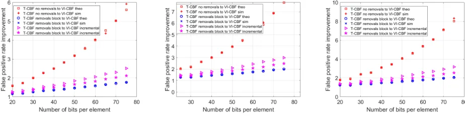
Fig. 2. L= 8,k= 4,r= 100, Left: False positive probability versus number of bits per element, Right: Improvement factor versus the VI-CBF.

Fig. 3. L= 4,kopt,r= 100, Left: False positive probability ratio versus the VI-CBF, Right: Optimum value ofk

Fig. 4. L= 8,kopt,r= 100, Left: False positive probability ratio versus the VI-CBF, Right: Optimum value ofk.

Fig. 5. False positive probability ratio versus the VI-CBF withr= 50,koptforL= 4(left),L= 8(middle),L= 16(right)

This figure clearly shows that the benefits of the T-CBF increase as the bits per element increases. Intuitively, a larger number of bits per element make more common the case that a counter, and in particular the counter adjacent to the one mapped by a hash function, has no elements. These are the cases for which T-CBF has potential to take advantage of for reducing false positives

through encoding of information in the adjacent counter. Let us now discuss in more detail the three different examined modes shown for the T-CBF:

• T-CBF no removals.

• T-CBF removals block.

The first (no removals) mode is the most strict one and accordingly achieves the highest accuracy. In this simple mode onlynelements are inserted and none of the them are removed. This means that no information located in adjacent counters is lost due to additional insertions/removals. Obviously, if there are no removals, there is no need to use a CBF as a simpler BF would provide the required functionality with a lower cost. Note, that the use of counters can enable future removals while the calculation of the probability of an error is valid before they appear. Moreover, this mode serves to illustrate the maximum benefit that can be obtained from the T-CBF and can also be a good approximation for applications in which there are few additional insertions and removals.

On the second mode (removals block), alln+relements are all first inserted and thenrof them are removed. This is a worst case for the T-CBF as all elements are stored in the filter at some point and all elements can be affected by the removals. Finally, the third case (removals incremental) tries to model a steady state in which the filter has a roughly constant load (number of represented elements) and elements are added and removed. In this configuration, elements inserted after a removal cannot be affected by it and thus the effect of removals is smaller than when they are done at the end in a block. Therefore, this second case is better than the removals in block and worse than the case of no additional insertion and removals. The results in Figure 2 show the impact of additional insertions and removals on the false positive probability. Clearly, this negative impact is smaller for lower values of r.

Let us now consider the matching of the false positive probabilities obtained by simulation with those of the theoretical estimates presented in the previous section. It can be seen that for the first two cases (no removals and removals block) the values match perfectly (to the simulation accuracy). This is expected as on average the theoretical formulas are accurate in those cases. In the last case, (removals incremental) the error is not negligible. Again this is expected as in this case the formula is just an approximation. An interesting observation is that the approximation tends to overestimate the false positive probability. This means that it can be used to provide an upper-bound on the false positive probability in a dynamic scenario. These observations hold for the other values of the different parameters that are not shown for brevity.

In a second set of simulations, our goal was to determine the value of the number of hash functions k that provides the lowest false positive probability for the different options and then observe the benefits of the T-CBF over the VI-CBF when both use their optimal settings (that can be different). The results for the different values ofLwhenr= 100are shown in Figures 3, 4. The left plot shows the improvement of the false positive rate for the T-CBF versus the VI-CBF and the right plot, the optimal values ofkfor the different options. Comparing Figure 2 with 4, it can be seen that for the optimal value of k the gain of the T-CBF is lower than when fixing k= 4. This can be explained as when the number of bits per element increases, if kdoes not change, there are more unused counters that the T-CBF can use to reduce the false positive probability. On the other hand, if we can change k, we can increase it so that the VI-CBF has less unused counters and a lower false positive probability. For

the T-CBF, there is a trade-off as increasing k makes the use of the adjacent counter less likely. Therefore we should expect the T-CBF to have lower values of the optimal k than the VI-CBF. This is in fact what happens as can be seen on the right plots in Figures 3, 4. For no removals and removals incremental, the T-CBF uses a value ofk that is in many cases one or two less than that of the VI-CBF. For the removals in block the difference is smaller. If we now look at L, we can see that the gains of the T-CBF increase slightly with L and the optimal values of k decrease. The decrease in k is expected as using larger increments implies more bits per counters and thus less number of counters for a given memory size.

The same set of simulations has been done when r = 50

and the results are summarized in Figure 5. The values do not change for the VI-CBF and for the T-CBF with no removals. For the T-CBF with removals in block or incremental, it can be observed that the gain over the VI-CBF increases. This matches our intuition as when less elements are inserted and removed, the T-CBF can more effectively use the adjacent counter. As the value ofrdecreases, the false positive probability decreases towards that of T-CBF with no removals. This means that the superiority of T-CBF over that of the VI-CBF is larger for applications on which the number of changes in the set is small, while in the general case, the probability for a false positive in the VI-CBF serves as an upper bound for that of T-CBF.

B. T-CBF Efficiency

After demonstrating the higher accuracy of the T-CBF we examine the efficiency of the filter. We compare the number of accessed counters and accessed memory words in applying filter operations, focusing on element insertions and queries. We also test the time in takes to perform these operations. As a baseline we again refer to the performance of the VI-CBF. We conduct the experiments using a real-life trace recorded on a single direction of an OC192 backbone link [16], and rely on a 64-bit mix hash function [17] of the IP 5-tuple to implement the requested hash functions. Evaluation was performed on a MacBook Pro with OS X Yosemite, 2.8 GHz Intel Core i7 processor with memory of 16GB, 1600 MHz DDR3.

20 25 30 35 40 45 50 55 60 0

4 8 12 16

bits per element

accessed

counters

VI-CBF T-CBF

(a) Accessed counters

20 25 30 35 40 45 50 55 60 0

4 8 12 16

bits per element

accessed

memory

w

ords

VI-CBF T-CBF

(b) Accessed memory words

20 25 30 35 40 45 50 55 60 0

0.2 0.4 0.6 0.8

bits per element

insertion

time

(µsec)

VI-CBF T-CBF

(c) Insertion time

Fig. 6. Comparison of the efficiency of the VI-CBF and T-CBF for theelement insertion operation.

20 25 30 35 40 45 50 55 60 0

0.5 1 1.5 2 2.5

bits per element

accessed

counters

VI-CBF T-CBF

(a) Accessed counters

20 25 30 35 40 45 50 55 60 0

0.5 1 1.5 2 2.5

bits per element

accessed

memory

w

ords

VI-CBF T-CBF

(b) Accessed memory words

20 25 30 35 40 45 50 55 60 0

0.05 0.1 0.15 0.2 0.25

bits per element

query

time

(µsec)

VI-CBF T-CBF

(c) Query time

Fig. 7. Comparison of the efficiency of the VI-CBF and T-CBF for theelement query operation.

Fig. 6 summarizes the efficiency results for the element insertion operation. First, Fig. 6(a) shows the number of accessed counters in an operation. For both filters, for a given bits per element value the number of accessed counters is fixed for all insertions, regardless of the filter state and the element identity. For the VI-CBF it is given by the number of hash functions and for the T-CBF by twice their number since two counters are accessed in each hash location upon insertion. Similarly, Fig. 6(b) presents the number of accessed memory words. This simply equals the number of hash functions for both filters since the T-CBF accesses pairs of counters sharing the same memory word. Last, Fig. 6(c) illustrates the average insertion time. The time is similar for both filters and no filter achieves faster insertions in all values. For both filters the time is highly affected by the hash function number. Interestingly, we can see that when both filters have the same function number (e.g., for 25 or 40 bits per element), the T-CBF time is longer by only roughly 10% (e.g., it increases from 0.2978 to 0.3238 for 25 bits per element and from 0.4338 to 0.4767 for 40 bits, all times in mircoseconds). This is in spite the fact the number of accessed counters is doubled (while the number of accessed words does not increase) and clearly shows the advantage of referring to two counters in the same word over accessing two arbitrary counters.

Fig. 7 presents the results for the query operation. We assume memory is accessed sequentially for the hash functions and query is completed whenever membership can be eliminated such that additional accesses are skipped. Moreover, for the T-CBF, upon measuring the number of accessed counters, we first access the

main counter in a memory word and the other counter is accessed only if its value is required. Fig. 7(a) shows the number of accessed counters. For both filters, this number is much smaller than the number of hash functions since the query can typically be answered based on the first accesses. For each of the filters the impact of the bits per element number on this value is small. Intuitively, the various number of hash functions imply similar distributions of the number of elements inserted to a counter and thus maintain similar probability to eliminate membership of a non-member element based on a single counter. The average number of accessed counters is in the range 1.54-1.80 for the VI-CBF and for T-CBF in the range 1.91-2.21, larger by 9-33%. This follows the T-CBF property to potentially consider a pair of counters in each hash location. Fig. 7(b) demonstrates that the additional information taken into account by T-CBF allows it to reduce the number of accessed memory words. This number decreases from 1.54-1.80 to only 1.42-1.56, with a reduction of 5.2%-18.9%. By Fig. 7(c) we can see that the reduction in the number of accessed memory words is translated to a similar reduction of 13.2%-24.1% in the query time.

VI. DISCUSSION

counter in the pair when possible. There are other possibilities to use those values that we have not explored. Some of them are discussed in the following. The study of the proposed scheme has focused on theDLvariant of the VI-CBF, in this section we also discuss its applicability when an arbitrary set D of increments is used. Finally parameter selection for the T-CBF is discussed. Alternative schemes: An option is to use increments

1,2, . . . ,2L−1, when a single element is stored in a counter, instead of just L, . . . ,2L−1. This would roughly double the probability to eliminate the membership based on such a counter. If another element is inserted, then the first 1,2, . . . ,2L−1

increment is transformed into a L, . . . ,2L−1increment before adding the new increment. A second alternative would be to group counters in trios instead of pairs. In that case, the unused counter range could be split into two so that each subrange is used to reduce the false positive probability of another element in the trio. For example subrange1, . . . , L/2can be used for one counter andL/2+1, . . . , L−1for the other. This provides larger flexibility to exploit unused counters but smaller reductions of the false positive probabilities as subranges are smaller. The complexity of insertions and lookups will also be larger.

Applicability to an arbitrary set of incrementsD:Although the analysis and evaluation has focused on theDL variant of the

VI-CBF, the proposed T-CBF can also be used to reduce the false positive probability of the other variants of the VI-CBF. In fact, for the case of D = {8,12,14,15} mentioned in [4], counter values1,2, . . . ,7,9,10,11,13are not used so that eleven values can be used to reduce the false positive rate for the other counter in the pair compared to the seven values of VI-CBF with D16. This seems to suggest that even larger reductions in the false positive rates can be achieved in this case.

Parameter Setting: We provide simple guidelines for the settings of parameters. We assume the number of elements that have to be represented, denoted by n is given. Moreover, an upper bound on the false positive probability is also provided. Based on these two, we find the minimal filter length m that allows such probability based on the formula from Theorem 1. If element removals are expected the formula from Theorem 3 can be used alternatively. The results for the VI-CBF (Figure 6 in [4]) suggested using the value L as 4 or 8. Similarly, based on the experiments in Section V, values of L as 8 or 4 achieve slightly large reductions of the false positive probability and should be the preferred configuration for the T-CBF, over others. Accordingly, we suggest to use one of these values as default. The set of variable increments is then [L,2L−1]. As discussed in Section IV-D for the selected parameter L, we allocate 4 +dlog₂(2L)e = 5 +dlog₂(L)e bits per counter. As shown in Theorem 4, a counter in T-CBF overflows exactly when a counter in the VI-CBF suffers from an overflow, thus the implied counter overflow probability is the same and negligible for practical settings. This preferred configuration uses 8 or 7 bit per counter that fit well with memory word sizes commonly used in computer systems.

VII. RELATEDWORK

In addition to the VI-CBF, other schemes have been suggested to improve the error-memory tradeoff of the CBF. In the evalu-ation of the T-CBF we focus on a comparison with the VI-CBF

as it is the most similar construction shown to outperform the above mentioned alternative constructions.

The regular CBF simply represents counters with a fixed number of bits per counter (typically four). More efficient representations have been suggested, benefitting from typically low counter values, not using the most significant bits of the counters. The ML-HCBF (MultiLayer Hashed CBF) [18] relies on a hierarchical compression where more bits are assigned to the least significant bits of the counters. Similarly, the VL-CBF (Variable Length CBF) [19] relies on Huffman coding to describe counters with a variable number of bits. Another approach is to rely on more than a single Bloom filter to improve accuracy. Lim et al. [20] proposed for the case of a finite universe maintaining two Bloom filters, representing a setS and its complement Sc_.

Since Bloom filters have no false negatives, if only one of the filters provides a positive answer, it is necessarily correct. If both provide a positive answer, both options should be examined.

Other studies [21], [22] suggested to reduce the false positives by allocating different number of hash functions to elements based on the query popularity. While the approach can be helpful for a skewed query distribution, maintaining the exact used number of hash functions per element can be challenging.

Another technique makes use of fingerprints [23], [24], [25]. Upon element insertion, a fingerprint is stored hash locations. This enables a careful examination of the counter upon a query. While the above approaches to reduce false positives maintain the property of no false negatives, other schemes allow false neg-atives to achieve this reduction in false positives. The Retouched Bloom filter [26] does so by clearing some of the bits that have earlier been set. Approaches are suggested to select the bits to be cleared, such as at randomly or in focusing on those that do not imply many false negatives. Likewise, the Generalized Bloom filter [27] maintains two groups of hash functions. Upon an element insertion, bits pointed by the first group are set and those by the second are cleared. A query of an element requires matching of some bits that have to be 0s and others that are 1s. Recent works described the Shifting Bloom Filter (ShBF), a data structure relying on encoding of auxiliary information in set representation for allowing membership, association, and multi-plicity queries using a reduced number of hash functions [28], [29]. For instance, auxiliary information can be encoded using an offset for the bits selected to be set in the filter. The ideas in the ShBF could also be potentially used to reduce the number of hash functions needed in the T-CBF. In [30] Yang et al. presented a data structure that supports multi-set membership queries of high accuracy through mapping elements to a high dimensional space to reduce hash collisions. Memory saving is achieved by a dimensional reduction representation similar to graph coloring. A similar approach was described in [31].

Kiss et al. suggested to carefully design hash functions so that false positives are completely avoided when the represented set is small [32]. The approach applies when elements are taken from a finite universe and its memory complexity is affected by the universe size and the maximal allowed set size.

VIII. CONCLUSIONS