Brand Imitation: A Dynamic-Game
Approach
1
Bertrand Crettez
2Naila Hayek
3Georges Zaccour
4September 5, 2018
1We would like to thank three Reviewers for their very helpful comments on two previous version
of this work. The third author’s research is supported by NSERC Canada, grant RGPIN-2016-04975. He also thanks CRED, Universit´e Panth´eon-Assas Paris II, for its hospitality.
2Universit´e Panth´eon-Assas, Paris II, CRED, [email protected].
3Universit´e Panth´eon-Assas, Paris II, CRED, [email protected]
Abstract
Brand imitation is a common practice that can take different forms, i.e., legal copying, as in the case of clones and knockoffs, or illegal, in the case of counterfeiting. We consider a scenario in which a producer enters the market with a “similar” product to the incumbent’s and we assess the impact of this entry on the incumbent’s strategies. A distinctive feature of our model is that it allows for brand dilution, which means that the original brand suffers due to imitation, and for brand enhancement, when the availability of the imitation product actually promotes the original brand.
We characterize and contrast the solutions for the scenario with entry and the benchmark case where no entry occurs, in a fully dynamic context and we examine the effect of a change in the date of entry on the entrant’s profit.
1
Introduction
Brand imitation, which can be defined as copying certain attributes (e.g., logo, design) of a well-established product, is common practice. The objective of this paper is to assess the impact of a third party offering a “similar” product on the incumbent’s strategies and outcomes.
Legal and illegal brand copying have been studied from different, not necessarily mutually exclusive, perspectives. At a macro level, one may wonder what is the impact of brand imi-tation on society. Schumpeter (1950) argued that imiimi-tation may inhibit innovation, and since innovation is needed in any society, monopolizing innovations through patents is justified. On the other hand, one may think that “good” imitations induce more competition, which in turn increases market efficiency and incites (innovative) firms to keep-up with quality.
In the above discussion, it is implicitly assumed that an imitation is a well-defined object. Except when the product is a counterfeit (a fake), which is a direct copy of a brand, defining precisely what constitutes an imitation is not a straightforward task from legal, economics and marketing standpoints. For instance, although trademark laws follow in general the same basic logic worldwide, that is, they aim at protecting the brand owner’s rights, they still differ in their details across countries and courts are judging cases on a one-by-one basis (Wilke and Zaichkowsky (1999)). Further, markets are full of copycats and lookalikes, e.g., private labels and store brands,1 which are not seen as illegal products. Scott-Morton and Zettelmeyer (2004) estimate that half of the store brands in national US supermarkets imitates a leader brand package at least in color, size and shape. In doing so, retailers want to signal that their products are “the same” as national brands while being affordable. Now, any given imitation (whether it is a copycat, lookalike or fake) may constitute a close substitute to an original brand for some consumers, while others may consider it as a very remote one. This is to recall that consumer typically looks beyond physical and tangible characteristics when drawing a perceptual (mental) map of competing brands.
In this paper, we are interested in looking at strategic interactions between a firm that sees its new product copied by another producer shortly after its introduction. Such situation is common in the apparel industry, where “fast-fashion” producers are able to replicate original styles and designs at high speed, on a large scale, and at low cost (Hemphill & Suk (2009)), and consequently, they sell them at a lower price than the original. Le Roux et al. (2016, p. 369) summarizes the problems that brand copying causes to an incumbent as follows: “Counterfeiting and imitation threaten hard-won competitive positions, dilute brand equity and undermine the status associated with products.” How should the incumbent react to its brand imitation? This is essentially the question we deal with in this paper. Now, brand equity (reputation or goodwill) and product’s status are firm’s assets that are acquired by investing in advertising and by implementing an appropriate pricing policy. Clearly, such assets cannot be built overnight but only over time. These features lead us to retain a dynamic game model and focus on advertising and pricing strategies to assess the impact of brand imitation on the incumbent.
Having in mind the apparel industry, we assume, not unrealistically, that entry (or im-itation) cannot be deterred. In fact, for an incumbent to strategically be able to deter
imitation, it is necessary that the entrant faces a (large) fixed cost, which is not the case re-tained here.2 To clearly position our contribution from the outset, we highlight the following
characteristics and assumptions of our model:
1. The product of interest is perishable as for, e.g., a fashion apparel. It is introduced by an incumbent at an initial time 0 and becomes obsolete at time T, that is, the selling season is [0, T].
2. An entrant has the know-how to copy the incumbent’s product and enters the market at an exogenously given date ∈ (0, T]. Consequently, we have a monopoly period followed by a duopoly period during which the two firms offer partially substitutable products.
3. The incumbent invests in advertising to raise its brand’s reputation, a variable that influences the current and future market size, and consequently, its demand and profit over time.
4. The entrant does not engage in any advertising activities, and its demand is determined by its price and the incumbent’s brand reputation. This assumption is meant to high-light the idea that purchasing, e.g., imitation Nike running shoes is driven by Nike’s reputation or goodwill, and of course, by the price of the two competing products.
5. After entry, the evolution of the brand reputation will not only depend on the incum-bent’s investment in advertising, but also be influenced by the imitator’s sales. More specifically, we shall consider two cases: (i) a negative effect (brand dilution) and (ii) a positive effect (brand or reputation enhancement). Brand dilution refers to the loss of reputation by a prominent brand and the devaluation of its exclusive features due to their use by a third party (here, the entrant). In the other case, the producer of the original brand gains in popularity (not necessarily directly through sales) thanks to the unintended free advertising done by the imitator. To illustrate, if one sees a “BlueBerry” or a “BleckBarry” mobile phone, one obviously immediately thinks of “BlackBerry”. A T-shirt displaying the slogan “Naik: Just do it” is clearly providing free advertising for Nike.3 Another example is “Hamossy” liquor offered in some
out-lets in China whose packaging clones Hennessy, the well-known brand of French cognac. Here, it is the Hennessy’s goodwill that is used to sell the alternative brand.
The above examples can be classified as knockoffs or clones, which are imitation products that are very similar to the original ones, but still use their own brand names. Another case of brand imitation is counterfeiting, which is an illegal activity. Cordell et al. (1996) define counterfeiting as “any unauthorized manufacturing of goods whose special characteristics are protected as intellectual property rights (trademarks, patents and copyrights) constitutes product counterfeiting.” Counterfeiters attempt to make products that are, at least at first
2There is a significant literature on entry deterrence (see the seminal paper by Milgrom and Roberts (1982)).
glance, indistinguishable from the famous genuine ones; otherwise, they would be less at-tractive to consumers. Our framework does not depend on whether or not the imitation is legal, and therefore can apply to copycats, lokkalikes and fakes. Consequently, we shall indifferently refer to the incumbent as the innovator, brand owner, or legal firm, and to the entrant as an imitator, counterfeiter, or competitor.
Our research questions are as follows:
1. How does the imitator’s entry affect the incumbent’s pricing and advertising strategies, before and after entry?
2. Are there circumstances under which the entrant benefits from delaying its entry?
To answer these questions, we adopt a finite-horizon dynamic game model. We believe this is the only framework that enables us to simultaneously account for the following fea-tures: (i) the sequential entry in the market of the two competitors; (ii) the fact that brand reputation is an asset built over time; (iii) the obsolescence of the product at the end of the selling season; and finally, (iv) the strategic interactions between the incumbent and the entrant.
Despite the prevalence of brand imitation, in both its legal and illegal forms,4the literature
looking at the dynamic strategic interactions between the incumbent and the entrant is sparse. While a central issue in counterfeiting is the impact on brand reputation and quality, the analysis is conducted using a static setting or, a two-period setup (see, e.g., Banerjee (2003, 2013), Qian (2012), Qian et al. (2014), and Zhang et al. (2012)). Although static and two-stage game models are helpful to enhance our understanding of strategic issues related to counterfeiting and brand imitation, they cannot fully capture the change in the state dynamics (e.g., brand reputation) before and after entry.
Our paper follows on Buratto et al. (2016) and Crettez et al. (2017), which are, to the best of our knowledge, the only papers dealing with brand imitation in a fully dynamic context. We share the following features with these two papers: (i) The differential game is played in two stages, monopoly and duopoly, with the entry date of the imitator being exogenously given. (ii) During the duopoly period, we seek a Nash equilibrium. Here and in Crettez et al., the information structure and the equilibrium are in feedback, whereas they are in open loop in Buratto et al. (iii) The incumbent chooses advertising and price levels, and the entrant chooses its price. In Buratto et al., it is additionally assumed that the entrant advertises the brand.
The major, significant difference between this paper and Buratto et al. (2016) and Crettez et al. (2017) is that here the evolution of the incumbent’s brand reputation also depends on the entrant’s sales during the duopoly period. By doing so, we actually want to measure the brand dilution mentioned in Le Roux et al. (2016). The owners of Channel bags who paid four-digit dollar prices to acquire them, will certainly feel a loss in status if they see Channel’s imitations all around. The status comes from rarity. We also want to consider, or at least not to exclude a priori, the case where imitation can benefit the incumbent. The examples
provided above, that is, “BlueBerry” and “BleckBarry” mobile phones, “Naik: Just do it”, and “Hamossy” cognac, may indeed end-up being free advertising to the original brands they are copying. We are postulating that their effects on brand’s equity can be well approximated by their sales, and consequently we can assess the impact on incumbent’s strategies. As we will see, the change in the dynamics specification introduced here affects the results considerably. Further, a noteworthy (technical) difference is that our optimization problems are not concave, and therefore, we could not resort to classical existence and uniqueness results, but had to develop new ones. We believe that this is a relevant contribution to the applied dynamic games literature in general.
The rest of the paper is organized as follows: In Section 2, we introduce the model, and in Section 3, we characterize the optimal and equilibrium solutions. We compare the incumbent’s before-entry strategies with and without brand imitation in section 4. Section 5 examines the effect of a change in the date of entry on the entrant’s profit. Section 6 briefly concludes.
2
Model
We consider a selling season defined by the time interval [0, T]. The initial date corresponds to the introduction of a new product by an incumbent (player I), and T to the date after which the product becomes obsolete because of, e.g., a change of season for fashion apparel, or the arrival of a new version for software. At an intermediate date ∈ (0, T], an entrant (player E) enters the market and offers an imitation of the incumbent’s product (or brand). Denote by pI(t) the price of the incumbent’s product at time t ∈ [0, T], and by pE(t) the
price charged by the entrant for its product at t∈ [, T].
Denote by B(t) the incumbent’s brand reputation (goodwill or brand equity). In the absence of brand imitation, the demand for the incumbent’s brand is given by
dI(t) = ˜αIB(t)−β˜IpI(t), t∈[0, T], (1)
where ˜αI and ˜βI are strictly positive parameters, and, in the scenario with brand imitation,
by
dI(t) =
˜
αIB(t)−β˜IpI(t), t∈[0, ), αIB(t)−βIpI(t) +γpE(t), t∈[, T],
(2)
dE(t) =αEB(t)−βEpE(t) +γpI(t), t∈[, T], (3)
where αj and βj are strictly positive parameters for j ∈ {I, E} and γ ≥0 with βj > γ, that
is, each demand is decreasing in own price and increasing in the competitor’s price, and the direct-price effect is greater than the cross-price effect.
The demands for the incumbent’s product are structurally different with and without brand imitation, that is, ˜αI 6=αI and ˜βI 6=βI, with ˜αI > αI and ˜βI < βI. Put differently,
setting pE(t) = 0 in the demand in the duopoly period does not yield the demand in the
reputation and that these demand functions are micro-founded.5 Furthermore, the market size for both players is proportional to the incumbent’s brand reputation. As alluded to in the introduction, this formulation is meant to highlight the fact that consumer demand for the imitated brand is driven by the reputation of the original/recognized brand.
Although the characterization of the solutions does not require additional assumptions on the demand parameter values, it seems intuitively reasonable to assume that (i) the owner of the brand benefits more from its brand reputation than does the imitator, i.e., αI > αE;
(ii) consumers of the clone brand are more sensitive to price than consumers of the original brand, i.e., βE > βI.
The manufacturer can increase the brand reputation by investing in advertising. After the possible entry of an alternative producer, the brand’s goodwill will depend on player I’s advertising effort and on the demand for the entrant’s product. The evolution of brand’s reputation is described by the following differential equations:
˙
B(t) =
ka(t)−σB(t), t ∈[0, ), ka(t) +ϕdE(t)−σB(t), t∈[, T],
B(0) =B0 >0, (4)
where a(t) is the advertising effort by the incumbent at time t, k > 0 is an efficiency (or scaling) parameter, ϕ is a parameter capturing the impact of the entrant’s demand on the incumbent’s brand reputation, and σ is the decay rate. A positive value of ϕ means that product’s reputation benefits from greater availability. Our assumption here is that this availability is actually free advertising for the incumbent’s brand. On the other hand, a negative value of ϕmeans that the reputation of the original product suffers from imitation, a phenomenon that is referred to as brand dilution.6
Following a large literature in differential games (see, e.g., the book by Jørgensen and Zaccour (2004) and the surveys by Huang et al. (2012) and by Jørgensen and Zaccour (2014)), we assume that the advertising cost is convex increasing and given by the quadratic function
CI(a) = ω
2a
2(t),
where ω is a positive parameter.
Setting the unit production cost equal to zero and assuming away discounting,7 the
in-5In Crettez et al. (2017), it is shown that these demand functions are obtained from the maximization of a representative consumer’s quadratic utility function.
6According to Qian (2014) “counterfeits have both advertising effects for a brand and substitution effects for authentic products, additionally the effects linger for some years. The advertising effect dominates the substitution effect for high-end authentic-product sales, and the substitution effect the advertising effect for low-end product sales.”
cumbent’s profit optimization program is as follows:
max
pI(t), a(t)
ΠI =
Z
0
pI(t)
˜
αIB(t)−β˜IpI(t)
−ω
2a
2
(t)dt +
Z T
pI(t) (αIB(t)−βIpI(t) +γpE(t))− ω
2a
2
(t)
dt
(5)
+sB(T),
subject to (4),
wheres is a nonnegative parameter, andsB(T) is the salvage value of the brand at T, which approximates the potential of future profits that the incumbent can obtain from selling other products under the same brand name.
The entrant’s optimization problem is defined as follows:
max
pE(t)
ΠE = max pE(t)
Z T
pE(t) αEB(t)−βEpE(t) +γpI(t)
dt. (6)
We assume that the entrant is myopic, that is, it optimizes its stream of profits ignoring the reputation dynamics. Such myopic behavior, which has been assumed in number of contributions in differential games (see, e.g., Benchekroun et al. (2009) and Mart´ın-Herr´an et al. (2012)), reflects the idea that the entrant does not care about the incumbent’s asset and is only interested in maximizing its payoff. In such a case, optimizing the above functional, while ignoring the state dynamics, is equivalent to solving the following static problem:
max
pE(t)
πE = max pE(t)
pE(t) αEB(t)−βEpE(t) +γpI(t)
, ∀t ∈[, T].
To assess the impact of brand imitation on the incumbent’s strategies, we consider as a benchmark the scenario where no such entry takes place. Here, player I solves the following finite-horizon optimal-control problem:
max
pI(t),a(t)
ΠI = max pI(t),a(t)
Z T
0
pI(t)
˜
αIB(t)−β˜IpI(t)
−ω
2a
2(t)dt+sB(T), (7)
˙
B(t) = ka(t)−σB(t), B(0) =B0.
We shall superscript the optimal price, advertising, and profit values with M (for monopoly). In the scenario where the imitator enters at time < T, the two firms play a finite-horizon differential game on the time interval [, T], with the incumbent maximizing
ΠI2 =
Z T
pI(t) (αIB(t)−βIpI(t) +γpE(t))− ω
2a
2
(t)
dt+sB(T),
subject to (4) and B() given,
function WI(, B()), which plays the role of a salvage value in its first-period optimization
problem given by
ΠI1 =
Z
0
pI(t)
˜
αIB(t)−β˜IpI(t)
−ω
2a
2(t)dt
+WI(, B()).
Comparing the outcomes of the two scenarios will allow us to measure the impact of brand imitation on the incumbent’s profit. We next study the case where there is entry.
3
Duopoly equilibrium
The incumbent’s optimization problem is in two stages: between 0 and , it is an optimal-control problem; between and T, a duopoly game is played and a Nash equilibrium is sought. To obtain a subgame-perfect Nash equilibrium (SPNE) in the two-stage problem, we first solve the second stage with B() as an initial value of the brand’s reputation.
3.1
The second-stage equilibrium
Denote by sj the strategy of player j ∈ {I, E}, and by Sj its strategy set. We suppose
that the duopoly game is played with feedback-information structure. That is, each player observes the state (t, B(t)) of the system and selects the control action according to the rule
uj(t) =sj(t, B(t)), where uI(t) = (pI2(t), a2(t))∈UI, uE(t) = (pE(t))∈ UE, and where Uj
is the control set of player j, and
sj(·,·) : (t, B(t))∈[, T]×R+ →Uj, j = 1,2.
We next recall the definition of a feedback-Nash equilibrium.8
Definition 1 A pair of strategies sNI , sNE is a feedback-Nash equilibrium if
ΠDI2(sNI , sNE) ≥ ΠDI2(sI, sNE), ∀sI ∈SI,
ΠDE(sNI , sNE) ≥ ΠDE(sNI , sE), ∀sE ∈SE.
To characterize a feedback-Nash equilibrium, denote by WI(t, B(t)) : [, T]×R+ → R
the incumbent’s value function. To save on notation, let
4E =
2βIαE +γαI
4βEβI−γ2 >0, 4I =
2βEαI+γαE
4βEβI−γ2 >0,
Ω =
ϕβE4E +4I
ϕγ3
4βEβI−γ2 −σ
,
Γ = 4βI42
I
k2
2ω +
ϕ2γ4β
E
(4βEβI−γ2)2
>0,
x(t) =
βI42
I
e2(T−t)
√
Ψ−1
1−e2(T−t)√Ψ
Ω + 1 +e2(T−t)√Ψ√
Ψ,
y(t) = se
Z T
t
Γ
βI42
I
x(i) + Ω
di
, z(t) =
Z T
t
Γ 4βI42
I
y2(i)di.
The following proposition gives the equilibrium solution of the duopoly game.
Proposition 1 Assume that
Ψ = Ω2−Γ≥0. (8)
(i) When Ω<0, there exists a unique interior non-oscillating feedback-Nash equilibrium, given for t∈[, T], by
pDI(t, B(t)) =4IB(t) +
∂WI(t, B) ∂B
2ϕγβE
4βEβI−γ2, (9)
pDE(t, B(t)) =4EB(t) +
∂WI(t, B) ∂B
ϕγ2
4βEβI −γ2, (10)
aD(t, B(t)) = k
ω(2x(t)B(t) +y(t)), (11)
where the value function WI is given by
WI(t, B(t)) =x(t)B2(t) +y(t)B(t) +z(t), (12)
The brand’s reputation trajectory is given by the solution of the differential equation
˙
BD(t) =
2x(t)k
2
ω +ϕβE4E −σ
B(t) +y(t)k
2
ω +
∂WI(t, B) ∂B
ϕ2γ2β
E
4βEβI−γ2, B() =B.
(ii) WhenΩ>0, there exists a unique interior non-oscillating feedback-Nash equilibrium, given by the above expressions if and only if
ln
Ω +√Ψ2
Γ
1
2√Ψ >2(T −). (13)
Proof. See Appendix.
1. The solution is interior whenϕ is negative. Indeed, in this case Ω is strictly negative, sox(t) is strictly positive for allt∈[, T].9 Further, notice that y(t) is strictly positive
for all t ∈ [, T], and so is z(t). In turn, this implies that the value function and its derivative are strictly positive for all t. Therefore, the prices and advertising are strictly positive for all t, with aD(T, B(T)) = ks
ω.
But when ϕ is strictly positive and Ω strictly positive the condition ln(Ω+
√
Ψ)2 Γ
1 2√Ψ >
2(T −) must be satisfied for x(t) to always be positive.10 Actually x(t) solves the
following differential equation (taken from the Riccati equations):
−x˙(t) =βI42
I + 2x(t)Ω +
Γ
βI42
I x(t)2,
with the terminal condition x(T) = 0. The necessary condition can be interpreted as follows. When ϕ is large and when the length of the interval T − is large, then, whatever the initial value ofx(),x(·) decreases at a high rate, and then it is impossible to satisfy the terminal condition x(T) = 0. The only way to do this is to start with
x() < 0. But this condition entails that ∂WI
∂B = 2x(t)B(t) +y(t) can be negative for
some high value of B(). Since aD = ωk∂W∂BI, this would require choosing a nil value for a(t), contradicting the fact that the equilibrium is interior.
2. The incumbent’s value function is quadratic in reputation,11 which is reminiscent of the
linear-quadratic structure of the differential game. Player I’s total equilibrium profit on [, T] is given by
WI(, B()) =x()B2() +y()B() +z().
As under condition (13) x(t) and y(t) are positive for all t, and in particular at , we have that the larger is the brand reputation at entry date, the larger the profit that the incumbent obtains during the duopoly period, irrespective of the sign of ϕ.
From now on, the conditions given in (8) and (13) are standing.
Before moving to the first-stage optimal solution, we look at two special cases, namely,ϕ= 0, which corresponds to the case where the entrant’s demand does not affect the incumbent’s brand reputation, and s = 0, which represents a scenario where the salvage value of B(t) is zero.
Corollary 2 Suppose that ϕ= 0, and assume that
σ2− 2βI42Ik2
ω ≥0. (14)
9The same holds whenϕis positive but small enough so that Ω is strictly negative. 10Notice that this condition implies thatϕis upper-bounded.
11We recall that the value function gives the optimal payoff that a player can achieve from any given state value (reputation and time). For instance, the value function evaluated at initial time 0 and initial reputation
Then, there exists a unique interior non-oscillating feedback-Nash equilibrium, given for
t ∈[, T], by
ˆ
pDI (t, B(t)) = 4IB(t), (15)
ˆ
pDE(t, B(t)) = 4EB(t), (16)
ˆ
aD(t, B(t)) = k
ω (2ˆx(t)B(t) + ˆy(t)), (17)
where the value function WI is given by
WI(t, B(t)) = ˆx(t)B2(t) + ˆy(t)B(t) + ˆz(t), (18)
with
ˆ
x(t) = βI4
2
I(f(t)−1)
−(1−f(t))σ+ (1 +f(t))
r
σ2− 2βI42Ik2 ω
,
ˆ
y(t) =se
Z T
t
2k2
ω xˆ(i)−σ
di ,
ˆ
z(t) =
Z T
t k2
2ωyˆ
2(i)di,
f(t) =e
2(T−t)
s
σ2−2βI42Ik2 ω
The brand’s reputation trajectory is given by the solution of the differential equation
˙
BD(t) =
2x(t)k
2
ω −σ
B(t) + ˆy(t)k
2
ω, B() =B.
Proof. It suffices to set ϕ = 0 in Proposition 1 to get the results. Note that in this case Ω = −σ <0, so the case of Ω>0 is irrelevant.
As one could expect, the results when ϕ = 0 are more compact than those obtained for ϕ 6= 0. In particular, we see that the prices are now simply proportional to brand’s reputation; the higher the brand reputation, the higher the price, which is in line with what it is typically observed in practice. As a consequence, the ratio of incumbent’s price to entrant’s price is constant over time. Indeed, we have
ˆ
pDI (t, B(t)) ˆ
pD
E(t, B(t))
= 4I
4E
= 2βEαI+γαE 2βIαE +γαI .
Corollary 3 Suppose that s = 0, and assume that
Ψ = Ω2−Γ≥0. (19)
(i) When Ω<0, there exists a unique interior non-oscillating feedback-Nash equilibrium, given for t∈[, T], by
˜
pDI(t, B(t)) = (2βEαI+γαE + 4x(t)ϕγβE)
B(t)
4βEβI−γ2, (20)
˜
pDE(t, B(t)) = 2βIαE +γαI+ 2x(t)ϕγ2
B(t)
4βEβI −γ2, (21)
˜
aD(t, B(t)) = k
ω(2x(t)B(t)), (22)
where the value function WI is given by
WI(t, B(t)) =x(t)B2(t) (23)
where we recall that
x(t) =
βI42
I
e2(T−t)
√
Ψ−1
1−e2(T−t)√Ψ
Ω + 1 +e2(T−t)√Ψ√
Ψ.
The brand’s reputation trajectory is given by the solution of the differential equation
˙
BD(t) =
2x(t)k
2
ω +ϕβE4E −σ
B(t) + ∂WI(t, B)
∂B
ϕ2γ2β
E
4βEβI−γ2, B() =B.
(ii) WhenΩ>0, there exists a unique interior non-oscillating feedback-Nash equilibrium, given by the above expressions if and only if
1
2√Ψln
Ω +√Ψ
2
Γ >2(T −).
Proof. It suffices to sets= 0 in the proof of Proposition 1 to get the results.
The cases = 0 corresponds to a situation where the incumbent is managing its brand as if there is no future after the selling season under consideration. We refer to this management as pessimistic decision-making. Few implications result from setting s= 0. First, the value function has only one (quadratic) term, a result that occurs when the objective functional in a differential games does not include a linear term. Second, for any given reputation level, the incumbent advertises less than in the case s 6= 0. Indeed, we have
aD(t, B(t))−˜aD(t, B(t)) = ky(t)
3.2
The first-stage optimal solution
The first-stage optimization problem of the incumbent is defined by
max
pI(t), a(t)
ΠI = max pI(t), a(t)
Z
0
pI(t)
˜
αIB(t)−β˜IpI(t)
− ω
2a
2(t)dt+W
I(, B()),
subject to the reputation dynamics
˙
B(t) = ka(t)−σB(t), B(0) =B0,
and where WI(, B()) is the salvage value giving the profit in the duopoly period as a
function of the reputation achieved at the starting date of that period.
The above optimization problem is a finite-horizon dynamic-optimization problem that can be solved equivalently using either the maximum principle or the Hamilton-Jacobi-Bellman approach. We shall follow the first approach as it happens to be easier to implement in our case.
Introduce the Hamiltonian
H pI(t), a(t), B(t), η(t)
=pI(t)
˜
αIB(t)−β˜IpI(t)
− ω
2a
2(t) +η(t) (ka(t)−σB(t)),
(24) where η(t) is the adjoint variable appended to the state dynamics. Before stating our results, we wish to highlight that the problem at hand is not concave. Indeed, it can be easily checked that the Hessian matrix, which is given by
∂2H
∂p2
I
∂2H
∂pI∂a ∂2H
∂pI∂B ∂2H
∂a∂pI ∂2H
∂a2 ∂
2H
∂a∂B ∂2H
∂B∂pI ∂2H
∂B∂a ∂2H
∂B2 =
−2˜βI 0 α˜I
0 −ω 0 ˜
αI 0 0
,
is not negative definite. The following proposition summarizes our results.
Proposition 2 Let t ∈[0, ). Assume that the incumbent’s price and advertising are upper-bounded as follows:
pI(t, B(t)) < p for all t and B(t), a(t, B(t)) < a¯ for all t and B(t),
with
p > α˜I
2˜βI
B0+
¯
ak σ
(25)
Then, there is a threshold ω(ϕ) such that for any ω > ω(ϕ) the interior solution is given by
pDI (B(t)) = α˜IB(t)
2˜βI , (26)
aD(t) =
k2˜βIη() (σ+v)ev(+t)−(σ−v)ev(−t)
+ ˜α2IB0 ev(2−t)−evt
2˜βIω((σ+v)e2v−(σ−v)) , (27)
BD(t) = 2˜βIη() (σ
2−v2) ev(+t)−ev(−t)
−α˜2IB0 (σ−v)evt−ev(2−t)(σ+v)
˜
where
v =
s
σ2− α˜ 2
I
2˜βI k2
ω.
Proof. See Appendix.
The following proposition gives the results in the no-entry benchmark scenario.
Proposition 3 The value function of the incumbent in the no-entry scenario is given by
VI(t, B(t)) =xM(t)B2(t) +yM(t)B(t) +zM(t),
where
xM(t) = α˜
2
I
4˜βI
(e2v(T−t)−1)
v−σ+ (v +σ)e2v(T−t)
≥0,
yM(t) = se
RT t
2xM(i)k
2
ω−σ
di >0,
zM(t) =
Z T
t k2
2ωy
2
M(i)di >0,
and the optimal solution is given by
pMI (B(t)) = α˜IB(t)
2˜βI , (29)
aM(t) =
k2˜βIs (σ+v)ev(T+t)−(σ−v)ev(T−t)
+ ˜α2IB0 ev(2T−t)−evt
2˜βIω((σ+v)e2vT −(σ−v)) , (30)
BM(t) = 2˜βIs(σ
2−v2) ev(T+t)−ev(T−t)
−α˜2IB0 (σ−v)evt−ev(2T−t)(σ+v)
˜
α2I((σ+v)e2vT −(σ−v)) (31).
Proof. See Appendix.
Given the linear-quadratic structure of the incumbent’s optimization problem, the above result is not surprising. Note that the three coefficients of the value function are strictly positive for allt, with the exception forT, wherexM(T) = 0. Further, the price is proportional to the brand’s reputation value and is stationary, that is, it does not depend explicitly on time. The advertising effort is strictly positive at all t∈[0, T]. The evolution over time of the advertising effort is given by
˙
aM(t) =
kν2˜βIs (σ+v)ev(T+t)+ (σ−v)ev(T−t)
−α˜2IB0 ev(2T−t)+evt
2˜βIω((σ+v)e2vT −(σ−v)) ,
with its sign depending on the parameter values. If the incumbent does not value its brand reputation at the terminal date, that is,s= 0, then ˙aM (t) is strictly negative and advertising
is monotonically decreasing over time.
Remark 1 Comparing(26)and(29)shows that the pricing policies during the time interval
[0, ) are the same. This does not mean that the trajectories of prices are the same, because the reputation stock will evolve differently in the two scenarios, that is, BM(t) 6=BD(t) for
4
Comparison of pre-entry strategies
In this section, we focus on the incumbent’s pricing and advertising policies during the interval [0, ], with the objective of assessing how entry affects the incumbent before it actually occurs. We first establish a general result, namely that the comparison of the pricing, advertising and reputation scenarios only depends on the difference between the shadow prices of brand reputation at the date of entry , in the absence and in the presence of the entrant. Recall that λM (), respectively ηD(), is the shadow price of brand reputation at date in the absence, respectively the presence, of the entrant.
Proposition 4 For all t∈[0, ], the differences in reputation, advertising, and price between the two scenarios are given by
BM(t)−BD(t) = 2˜βI(σ
2−v2) ev(+t)−ev(−t)
˜
α2I((σ+v)e2v−(σ−v)) λ M
()−ηD(),
aM(t)−aD(t) = 2k ˜
βI (σ+v)ev(+t)−(σ−v)ev(−t)
2˜βIω((σ+v)e2v−(σ−v)) λ M
()−ηD(),
pMI (t)−pDI (t) = (σ
2−v2) ev(+t)−ev(−t)
˜
αI((σ+v)e2v−(σ−v))
λM()−ηD(),
and therefore,
sign BM(t)−BD(t)
= sign aM(t)−aD(t)
=sign pMI (t)−pDI (t) ,
= sign λM()−ηD() .
Proof. Straightforward computations lead to the results.
The above proposition bears few interesting messages. First, it shows that comparing the incumbent’s decisions during the whole time interval [0, ] boils down to just comparing two numbers, i.e., λM() andηD(). The implication is that the two price trajectories never cross
each other. This implies that during the pre-entry period [0, ], the price in the no-entry scenario (pMI (t)) is either always higher than or equal to, or always lower than or equal to, the price in the entry scenario (pD
I (t)). The same statement can be made for advertising
and reputation.
Second, the evolution over time of these differences also depends on the sign of λM()−ηD(). Indeed, it suffices to differentiate these differences with respect to time to obtain
˙
BM(t)−B˙D(t) = 2˜βIν(σ
2 −v2)v ev(+t)+ev(−t)
˜
α2I((σ+v)e2v−(σ−v)) λ
M()−ηD() ,
˙
aM(t)−a˙D(t) = 2k ˜
βIv (σ+v)ev(+t)+ (σ−v)ev(−t)
2˜βIω((σ+v)e2v−(σ−v)) λ
M()−ηD() ,
˙
pMI (t)−p˙DI (t) = (σ
2−v2)v ev(+t)+ev(−t)
˜
αI((σ+v)e2v−(σ−v))
λM()−ηD() .
Clearly, all coefficients of λM()−ηD() are positive, and hence, the result. Finally, at the initial instant of time, we have pM
that BM (0) = BD(0) = B0. However, the two advertising levels are not the same at the
initial date, with the difference between them being given by
aM(0)−aD(0) = 2kve
v
ω((σ+v)e2v−(σ−v)) λ
M()−ηD() .
Let us now consider the expressionλM()−ηD(). Recall that
λM() = ∂VI
∂B B
R(),
= 2xM()BM() +yM(), (32)
ηD() = ∂WI
∂R B
D(),
= 2x()BD() +y(). (33)
Now, from Proposition 4, we also have
BM(t)−BD(t) = 2˜βI(σ
2−v2) ev(+t)−ev(−t)
˜
α2I((σ+v)e2v−(σ−v)) λ M
()−ηD().
Let g() be defined as
g() = 2˜βI(σ
2−v2) (e2v−1)
˜
α2I((σ+v)e2v−(σ−v)).
Using the expressions of λM() and ηD() in (32) and (33), we have
λM()−ηD() = 2B
D() (x
M()−x()) +yM()−y()
1−2xM()g()
. (34)
The above difference depends in a highly non-linear way on all model’s parameters. (The full expression can be seen in the proof of Proposition 5.) Analytically, we can determine the sign of this difference only in the specific case where advertising is very expensive (the cost parameter ω is very large) and ϕ= 0, that is, the entrant’s demand does not affect the brand reputation dynamics.
Proposition 5 Assume ϕ= 0. Then, we havelimω→+∞(λM()−ηD())>0.
Proof. See Appendix.
By a continuity argument, this result can be extended to all ϕ in a neighborhood of 0. Thus, when the absolute value of ϕ is low enough, and ω is high enough it follows from Proposition 4 that
sign BM(t)−BD(t) = sign aM (t)−aD(t) =sign pMI (t)−pDI (t) = sign λM()−ηD()
>0.
How general is this result? The short answer is that it is not. To show that the difference
λM()−ηD() can assume any sign, it is in fact sufficient to provide 3 numerical examples.
In the examples to follow, all conditions imposed on the parameters are satisfied and the solutions are meaningful, i.e., we have positive prices, advertising and demands.
Our model has 15 parameters, namely:
Demand parameters : α˜I,β˜I, αI, βI, αE, βE, γ;
Advertising parameters : ω, k; Brand reputation parameters : B0, ϕ, σ, s;
Dates : T, .
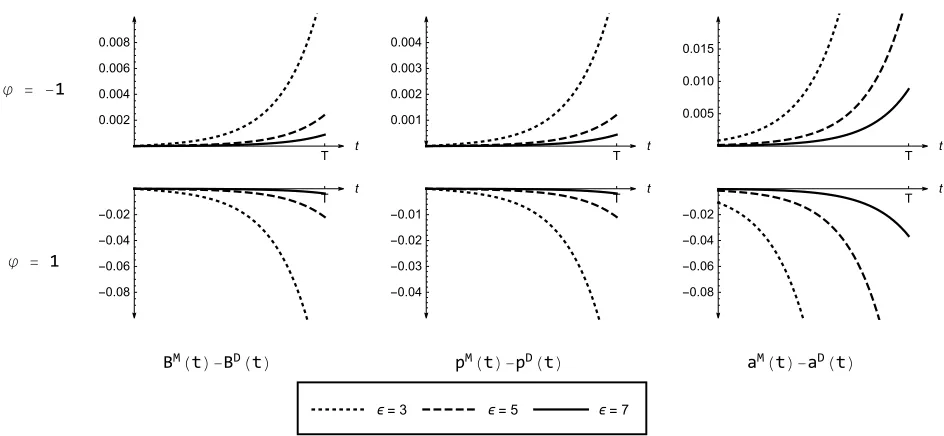
To start with, we fix the values of 13 of the above parameters as follows:
˜
αI = 100,β˜I = 0.5, αI = 85, βI = 1.1, αE = 80, βE = 1, γ = 0.9, (35) ω = 10, k = 0.01, B0 = 10, σ = 0.5, s= 1, T = 10,
and consider three entry dates, that is, = 3,5,7, to be interpreted as early, intermediate and late entry date, respectively. The only left parameter is the impact of entrant’s demand on reputationϕ. Figure 1 exhibits the results for two values ofϕ, namely, one negative (−1) and one positive (+1). Clearly, we have
sign BM(t)−BD(t)
=sign aM(t)−aD(t)
= pMI (t)−pDI (t)
=−signϕ,
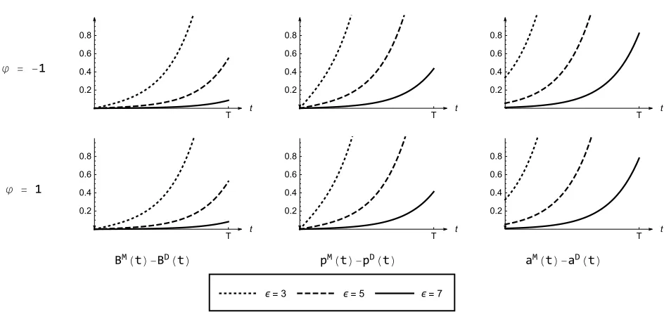
that is, the sign of the differences in brand reputation, advertising efforts and prices is the opposite of the sign ofϕ. Now, changing the value of ˜αI to 10, while keeping everything else
as before, yields the results in Figure 2, we get
sign BM(t)−BD(t)=sign aM(t)−aD(t)= pMI (t)−pDI (t)>0.
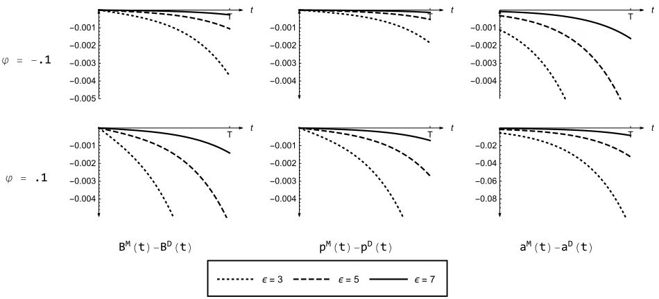
Here, the incumbent will price and advertise at a higher level before entry, independently on whether the entrant will harm or not its brand reputation. (Note that the numerical values are close, but not the same, for ϕ negative and positive are close.) Finally, we change in Figure 3 the values of σ to 0.3 andϕto ±0.1 (the value of ˜α is reverted to 100), and obtain the opposite result that the one above, i.e.,
sign BM(t)−BD(t)=sign aM(t)−aD(t)= pMI (t)−pDI (t)<0.
For this parameter constellation, the incumbent will price and advertise at a lower level before entry, independently on whether the entrant will harm or not its brand reputation.
Based on these illustrations, and many others that we ran, we reach two conclusions.12
First, the impact of imitation on the incumbent’s before-entry strategies cannot be deter-mined utterly and is definitely an empirical matter. For instance, we clearly see by comparing the results in Figures 1 and 2 that the market size ˜αI matters to the outcome, both
qual-itatively and quantqual-itatively. Comparing Figures 2 and 3, we can observe the impact on the results of two parameters that influence the brand dynamics (ϕ and σ). Second, the later the entry date, the lower is the difference between the trajectories. Interestingly, in all cases, we obtain that when = 7, which still leaves 30% of the planning horizon to come, the differences in brand reputation, prices and advertising efforts become negligible.
φ = -1
T t 0.002
0.004 0.006 0.008
T t 0.001
0.002 0.003 0.004
T t 0.005
0.010 0.015
φ = 1
T t
-0.08 -0.06 -0.04 -0.02
T t
-0.04 -0.03 -0.02 -0.01
T t
-0.08 -0.06 -0.04 -0.02
BM(t)-BD(t) pM(t)-pD(t) aM(t)-aD(t)
ϵ=3 ϵ=5 ϵ=7
Figure 1: Impact of ϕfor different entry cases, Case 1
5
Entrant’s profit and the date of entry
An important assumption of our analysis is that the date of entry is exogenous. As we have mentioned, this may reflect the time needed by the imitator to learn how to produce the good supplied by the legal firm. To assess the relevance of this assumption, it is interesting to see how the entrant’s profit varies with a change in . As it is shown in the Appendix (proof of Proposition 6), it is not possible to determine the sign of the derivative ∂ΠDE
∂ for all parameter
values. The fact that the sign of ∂ΠDE
∂ is indeterminate in general can be explained as follows.
First of all, an increase in directly increases the value of the legal firm goodwill at date
(the length of the monopoly period being marginally higher). This, in turn, affects positively the entrant’s profit. But, on the other hand, an increase in decreases the entrant’s profit since it operates during fewer time. Since the two effects play in opposite directions the sign of ∂ΠDE
∂ is indeterminate. However, we could establish the following analytical result:
Proposition 6 When w is very high, the entrant’s profit is a decreasing function of the date
of entry.
Proof. See Appendix.
The above result shows that when ω is high enough, the entrant is better off when the date of entry occurs early, which is intuitive. Whenω is large, it is costly for the legal firm to build its reputation. Thus increasing the monopoly period will not contribute much to the reputation building, but will decrease the opportunity of the entrant to make more profit. This is why in this case increasing the date of entry decrease the entrant’s profit.
To further investigate the impact of entry date on entrant’s profit, we conducted a large series of numerical experiments adopting the following steps:
φ = -1
T t
0.2 0.4 0.6 0.8
T t
0.2 0.4 0.6 0.8
T t
0.2 0.4 0.6 0.8
φ = 1
T t
0.2 0.4 0.6 0.8
T t
0.2 0.4 0.6 0.8
T t
0.2 0.4 0.6 0.8
BM(t)-BD(t) pM(t)-pD(t) aM(t)-aD(t)
ϵ=3 ϵ=5 ϵ=7
Figure 2: Impact of ϕfor different entry dates, Case 2
Step 2: Let∈ {0.1×T,0.2×T, . . . ,0.9×T}. Compute the entrant’s profit for all values
, and identify the instances where a larger leads to higher profits.
Step 3: Change one of the parameter value at a time with respect to its base case value and repeat the computation in Step 2.
Note that in this process, only the cases with positive prices, advertising and demands are retained. Based on these numerical experiments, we state the following:
Conjecture. The entrant is better off entering at the earliest possible date.
Put differently, we could not identify (numerically) a single instance where the entrant is better off delaying its entry. This result tends to say that assuming exogenous entry date is not a severe hypothesis as what really matter in our setup is the time the entrant needs to learn how to produce the good.
6
Managerial implications and concluding remarks
Brand imitation is common practice in retail industries and is well-documented since the mid-1800s (Wilke and Zaichkowsky (1999)). When imitation is illegal (counterfeiting), the owner of the brand can count on policies and policing to combat it. Luxury and well-established brands devote a considerable amount of money and effort to deter counterfeiting. For instance, LVMH assigns approximately 60 full-time employees to anti-counterfeiting (Qian (2014), whereas Lego@ has a team of lawyers who handle 30 to 40 cases of brand imitation
φ = -.1
T t
-0.005 -0.004 -0.003 -0.002 -0.001
T t
-0.004 -0.003 -0.002 -0.001
T t
-0.004 -0.003 -0.002 -0.001
φ = .1
T t
-0.004 -0.003 -0.002 -0.001
T t
-0.004 -0.003 -0.002 -0.001
T t
-0.08 -0.06 -0.04 -0.02
BM(t)-BD(t) pM(t)-pD(t) aM(t)-aD(t)
ϵ=3 ϵ=5 ϵ=7
Figure 3: Impact of ϕfor different entry dates, Case 3
brands, because their reputation is a main driver of their demand and there is room for high profit margins. By focusing on pricing and advertising (and the resulting brand reputation), we are actually dealing with the incentives behind imitations and the main policies that are at the incumbent disposal to react to this form of competition. Although imitation harms the brand reputation in general, we did not limit our model to this negative impact, but also analyzed the case where the incumbent may actually benefit from imitation.
The main takeaways from this paper are as follows: (i) In the absence of fixed cost, the incumbent cannot deter entry, and therefore the problem becomes one of how to accommo-date/combat the competitor; (ii) The entrant will indeed enter the market at the first possible opportunity, that is, as soon as the know-how and logistics for copying and producing the imitation are in place; (iii) The impact of brand imitation is felt before and after entry. That is, entry affects the incumbent’s pricing and advertising strategies over time, which in turn influences the salvage value of the brand, implying an impact well beyond the selling season; (iv) The before-entry strategies depend on all parameter values, and not only, as one could expect, on how entrant’s demand affects the reputation of the incumbent’s brand. The later entry occurs, the less it affects before-entry decisions, which is intuitive.
7
Appendix: Proofs
Proof of Proposition 1
Recall the change of notation introduced before, namely:
4E =
2βIαE +γαI
4βEβI−γ2 >0, 4I =
2βEαI+γαE
4βEβI−γ2 >0,
Ω =
ϕβE4E +4I
ϕγ3
4βEβI−γ2 −σ
,
Γ = 4βI42
I
k2
2ω +
ϕ2γ4β
E
(4βEβI−γ2)2
>0,
Ψ = Ω2−Γ.
Let pI(t, R) be given, then the entrant’s problem is a static maximization problem, and the
first-order optimality condition is
αEB +γpI(t, B)−2βEpE(t, B) = 0. (36)
Given pE(t, B), the incumbent’s problem is a dynamic optimization problem.
Denote byWI the incumbent’s value function. For all (t, B)∈[, T]×R+, the
Hamilton-Jacobi-Bellman (HJB) equation reads as follows:
−∂WI(t, B)
∂t = maxpI,a
{pI(αIB−βIpI+γpE(t, B))− ω
2a
2
+∂WI(t, B)
∂B (ka+ϕdE(t, B)−σB)},
with the terminal conditionWI(T, B) =sB. Assuming an interior solution and maximizing
the right-hand side of the HJB equation yields
αIB+γpE(t, B)−2βIpI(t, B) +ϕγ
∂WI(t, B)
∂B = 0. (37)
a(t, B) = k
ω
∂WI(t, B)
∂B . (38)
Using (36) and (37), we get the following pricing policies:
pE =
γαI+ 2βIαE
4βEβI−γ2 B+
∂WI(t, B) ∂B
ϕγ2
4βEβI−γ2 =4EB+
∂WI(t, B) ∂B
ϕγ2
4βEβI−γ2,
pI =
γαE + 2βEαI
4βEβI−γ2 B+
∂WI(t, B) ∂B
2ϕγβE
4βEβI−γ2 =4IB+
∂WI(t, B) ∂B
2ϕγβE
4βEβI−γ2.
Consequently, the demand of the entrant is
dE =βE4EB+
∂WI(t, B) ∂B
ϕγ2βE
4βEβI−γ2.
Substituting for the prices and advertising in the HJB equation, we obtain
−∂WI(t, B)
∂t =βI4
2
IB
2+ ∂WI(t, B)
∂B ΩB+
Γ 4βI42
I
∂WI(t, B) ∂B
2
Given the linear-quadratic structure of the game, we make the informed guess that the value function is of the form
WI(t, B) = x(t)B2+y(t)B+z(t),
with WI(T, B) =sB for all nonnegativeB.
The following expressions will be useful later on:
∂WI(t, B)
∂t = ˙x(t)B
2
+ ˙y(t)B+ ˙z(t),
∂WI(t, B) ∂B
2
= 4x(t)2B2+y(t)2+ 4x(t)y(t)B.
Plugging these expressions into the HJB equation, we get
− x˙(t)B2+ ˙y(t)B+ ˙z(t)
= βI42
IB
2+ (2x(t)B+y(t)) ΩB
+ Γ 4βI42
I
4x(t)2B2+y(t)2+ 4x(t)y(t)B,
for all t and B. By identification, we obtain
−x˙(t) = βI42
I+ 2x(t)Ω +
Γ
βI42
I
x(t)2 (39)
−y˙(t) = Γ
βI42
I
x(t)y(t) + Ωy(t), (40)
−z˙(t) = Γ 4βI42
I
y(t)2. (41)
Moreover, from the conditionWl(T, B) = x(T)B2+y(T)B+sz(T) = sB for all nonnegative B, we have x(T) = 0, y(T) =s and z(T) = 0.
We solve the above system recursively. Let us start with equation (39), which is a Ricatti equation. Consider the differential equation:
˙
z(t) = 2ι(t)z(t) +κ(t)−ρ(t)z(t)2, (42)
where ι(t), κ(t) and ρ(t) are continuous functions of t. Let us now consider the system
˙
m =ι(t)m+κ(t)n, (43)
˙
n =ρ(t)m−ι(t)n. (44)
We can check that if m(t) and n(t) are a solution to the above system (with t ∈ (t0, t1)),
n(t) 6= 0, then z(t) = m(t)/n(t) is a solution to equation (42). In our problem, we have
κ(t) =−βI42
I,ρ(t) =
Γ
βI42I
, ι(t) =−Ω. Therefore, we want to solve the following differential system:
˙
m
˙
n
=
−
Ω −βI42
I
Γ
βI42I
Ω
m n
(45)
The Eigenvalues of the above matrix are solutions to the equation
u2 = Ψ,
that is,
u1 =
√
Ψ and u2 =−u1.
The corresponding eigenvectors are respectively
1 m1 2 = 1
−Ω+√Ψ
βI42I ! and 1 m2 2 = 1
−Ω−√Ψ
βI42I
!
.
Now, the solution of the differential system (45) can be written as
m(t)
n(t)
=c1
1
m12
e
√
Ψt+c
2
1
m22
e−
√
Ψt
To find c1 and c2 we solve the following system:
0 1 = e √
ΨT e−√ΨT m1
2e
√
ΨT m2 2e
−√ΨT ! c1 c2 .
We find that
c1 c2 = 1 m2 2 −m12
−e−
√ ΨT e √ ΨT ! ,
where m2
2−m12 = 2√Ψ
βI42I
. Therefore,
x(t) = c1e
√
Ψt+c
2e−
√
Ψt
c1m12e
√
Ψt+c
2m22e−
√
Ψt =
βI42
I
e2√Ψ(T−t)−1
(1−e2√Ψ(T−t))Ω + (1 +e2√Ψ(T−t))√Ψ.
Notice that that when ϕ ≤ 0, we have Ω <0 so x(t) >0 for all t ∈ [, T]. The same holds when ϕ > 0 but small enough so that Ω < 0. But when ϕ > 0 and Ω > 0, the condition
ln(Ω+
√
Ψ)2 Γ
1
2√Ψ >2(T −) ensures that x(t)>0 for all t∈[, T].
Now, consider the differential equation iny(t). We readily see that
y(t) = s·e
Z T
t
Γ
βI42
I
x(i) + Ω
di .
Notice that y(t)>0 for all t. We finally obtain
z(t) =
Z T
t
Γ 4βl42
I
y2(i)di,
Now, a(t) = ωk(2x(t)B(t) +y(t)) and
˙
B(t) =ka(t) +ϕdE(t)−σB(t), (46)
=
k2
ω2x(t) +ϕβE4E −σ
B(t) + k
2
ωy(t) +
∂WI(t, B) ∂B
ϕ2γ2βE
4βEβI−γ2. (47)
We now show that (21) and a(t) = ωk∂WI(t,R)
∂B define a Nash equilibrium in the
second-stage counterfeiting scenario. Given pI(t, B) in (20), we have that pE(t, B) in (21) solves the
counterfeiter’s problem since its payoff is concave with respect topE. GivenpE(t, B) in (21),
we have seen that pI(t, B) and a(t, B) solve the legal firm’s problem. Hence, the result.
Proof of Proposition 2
Proposition 1 ensures the existence of a feedback-Nash equilibrium in the second stage. The same proposition yields the expression of the value function associated to the incumbent’s problem in the second stage. Now, assume for a while that there exists ω such that
ω > k a
(
˜
α2I
2˜βIσ(B(0) + ka
σ ) +B∈[0,sup sup t∈[0,]{B(0)e−σt+ka
Rt
0eσ(u−t)du}]
∂WI
∂B (, B;ϕ, ω) )
. (48)
The proof of the proposition is in four steps.
Step 1. We prove the existence of a solution to the incumbent’s problem with arbitrary bounds on the controls. Consider the following constrained problem (II):
max
pI(t), a(t)
ΠI = max pI(t), a(t)
Z
0
pI(t)
˜
αIB(t)−β˜IpI(t)
− ω
2a
2(t)dt+W
I , B()
,(49)
˙
B(t) = ka(t)−σB(t), B(0) =B0,
with 0 ≤a(t)≤a, and 0≤pI(t)≤p, where a andp are positive real numbers defined in the
statement of the proposition.
The existence follows from Filippov’s Theorem (see Filipov (1962)).
Step 2. Let us show that the solution is interior, i.e., satisfies 0 < pI(t) < p and
0< a(t)< a for all t.
The solution to problem (II) maximizes the following Hamiltonian at each datet:
H =pI(t)
˜
αIB(t)−β˜IpI(t)
− ω
2a
2(t) +η(t) (ka(t)−σB(t))
Therefore, the next first-order conditions must be satisfied:
∂H ∂pI
= 0 ⇐⇒ α˜IB(t)−2˜βIpI(t) +θ(t)−ζ(t) = 0, (51)
∂H
∂a = 0 ⇐⇒ −ωa(t) +kη(t) +ξ(t)−ψ(t) = 0, (52)
˙
η(t) =−∂H
∂B =−α˜IpI(t) +η(t)σ, η() = ∂WI
∂B (, B()), (53)
˙
B(t) = ∂H
∂η =ka(t)−σB(t), B(0) =B0, (54) pI(t)≥0, θ(t)≥0, θ(t)pI(t) = 0, (55) a(t)≥0, ξ(t)≥0, ξ(t)a(t) = 0, (56)
pI(t)≤p, ζ(t)≥0, ζ(t)(p−pI(t)) = 0, (57) a(t)≤a, ψ(t)≥0 ψ(t)(a−a(t)) = 0. (58)
Solving forB(t), we have
B(t) = B0e−σt+k
Z t
0
eσ(u−t)a(u)du > B0e−σt >0. (59)
Note that B(t) is always positive.
• Now let us show that 0< pI(t)< p, for all t.
Assume thatpI(t) = 0. Then,ζ(t) = 0 and the first-order condition (51) writes ˜αIB(t) + θ(t) = 0. Since θ(t)≥0 and B(t) is positive, we get a contradiction.
Now let us show that pI(t) < p. Assume that pI(t) = p for some t. Then, θ(t) = 0, and
from equation (51), we have pI(t) = p= α˜IB(t)
−ζ(t)
2˜βI . Since ζ(t)≥0, it follows that p <
˜
αIB(t)
2˜βI .
From equation (59) and the fact that a(t)≤a, we have
p < α˜I
2˜βI
B0e−σt+ka
Z t
0
eσ(u−t)du
= α˜I 2˜βI
B0e−σt+
ka σ (1−e
−σt)
, (60)
< α˜I
2˜βI(B0+ ka
σ ), (61)
which contradicts (25). Therefore, we have pI(t) = α˜I2˜Bβ(t) I
for all t.
• 0< a(t)< afor all t.
Assume by way of contradiction that there is some t at which a(t) = 0. Then, ψ(t) = 0 and (52) can be written askη(t) +ξ(t) = 0. Sinceξ(t)≥0,therefore we haveη(t) = ξ(kt) ≤0.
Let us show that t 6= . Indeed, η() = ∂WI
∂B (, B()). Under our assumption ∂WI
∂B is
positive. Since B0 >0, we have seen that B(t) is always positive.
Now solving for η(t) from (53) (and using pI(t) =
˜
αIB(t)
2˜βI
) we get
η(t) = eσt
Z
t
e−σu α˜
2
I
2˜βIB(u)du+e
−σ η()
. (62)
Now assume again by way of contradiction that there is a datetat whicha(t) =a. Then,
ξ(t) = 0 and we must have −ωa+kη(t)− ψ(t) = 0. Therefore, kη(t) = ωa +ψ(t), or
η(t)≥ ωa
k . Now from (59), we have
B(t) =B0e−σt+k
Z t
0
eσ(u−t)a(u)du,
≤B0e−σt+km
Z t
0
eσ(u−t)du,
=B0e−σt+
ka σ (1−e
−σt),
≤B0+
ka σ .
Using (62) we get
ωa
k ≤η(t)≤e σt
Z
t
e−σu α˜
2
I
2˜βI(B0+ ka
σ )du+e
−ση()
,
= α˜
2
I
2˜βIσ(B0+ ka
σ )(1−e
σ(t−)) +eσ(t−)η(),
< α˜
2
I
2˜βIσ(B0+ ka
σ ) +η() =
˜
α2I
2˜βIσ(B0+ ka
σ ) + ∂WI
∂B (B()),
≤ α˜
2
I
2˜βIσ(B0 + ka
σ ) + B∈[0,sup sup t∈[0,]{B0e−σt+ka
Rt
0eσ(u−t)du}]
∂WI
∂B (, B).
But this last inequation contradicts the assumption (48).
Step 3. We can check that (26)-(28) is the interior solution of the first-order conditions (when θ(t) = ζ(t) = ξ(t) = ψ(t) = 0) provided that σ2 ≥ α˜2I
2˜βI k2
ω. Indeed, the first-order
optimality conditions become
˜
αIB(t)−2˜βIpI(t) = 0⇔pI(t) =
˜
αIB(t)
2˜βI ,
−ωa(t) +kη(t) = 0 ⇔a(t) = η(t)k
ω ,
˙
η(t) = −∂H
∂B =−α˜IpI(t) +η(t)σ, η() = ∂WI
∂B (, B()),
˙
B(t) = ∂H
∂η =ka(t)−σB(t), B(0) =B0.
Substituting for the controls in the state and adjoint equations yields the following linear differential system:
˙
η = ση− α˜
2
I
2˜βIB, η() = ∂WI
∂B (, B()),
˙
B = k
2
This system can be written ˙Y =AY,whereY =
η B
, ˙Y =
˙ η ˙ B
andA= σ −
˜
α2
I
2˜βI k2
ω −σ
!
.
Sinceσ2 ≥ α˜ 2
Ik2
2˜βIω, the two real eigenvalues arev and−v,wherev = q
σ2− ˜α2I
2˜βI k2
ω and the
corresponding eigenvectors are
V1 =
1 2˜βI(σ−v)
˜
α2I
, V2 =
1 2˜βI(σ+v)
˜
α2I
.
Therefore, the general solution of the linear-differential system is given by
Y(t) =r1evtV1+r2e−vtV2,
that is,
η(t) = r1evt+r2e−vt,
B(t) = r1
2˜βI(σ−v) ˜
α2I e vt
+r2
2˜βI(σ+v) ˜
α2I e
−vt .
Further,r1 and r2 are uniquely determined (using Cramer’s rule for example) so that the
solution satisfies the boundary conditions η() = ∂WI
∂B (, B()) andB(0) = B0. We obtain
r1 =
2˜βI(σ+v)η()ev−α˜2IB0
2βI((σ+v)e2v−(σ−v)), (63)
r2 =
e2vα˜2
IB0−2˜βI(σ−v)η()ev
2˜βI((σ+v)e2v−(σ−v)) . (64)
Consequently, we get
B(t) = r1
2˜βI(σ−v) ˜
α2I e vt+r
2
2˜βI(σ+v) ˜
α2I e
−vt,
pI(t) =
˜
αIB(t)
2˜βI =r1
(σ−v) ˜
αI
evt+r2
(σ+v) ˜
αI
e−vt,
a(t) = (r1e
vt+r
2e−vt)k
ω .
Substituting forr1 and r2 into B(t),pI(t) anda(t), we obtain (26)-(28).
Step 4. To guarantee that the solution of the first-order conditions exists and is unique, the following equation must have a unique solution in B():
BD() = 2˜β
∂WI ∂B (B
D()) (σ2−v2) (e2v−1) +B
0((σ+v)ev−(σ−v)ev) ˜α2I
˜
αI2((σ+v)e2v−(σ−v))
, (65)
= 2∂WI
∂B (B D
()) ˜
βI
˜
α2I
(e2v−1)(σ−v) e2v−σ−v
σ+v
+ 2B0ve
v
(σ+v) e2v− σ−v σ+v
where ∂WI
∂B (B) = 2x(t)B+y(t). This equation has a positive solution B
D() if, and only if,
4x() ˜
βI
(˜αI)2
(e2v−1)(σ−v) e2v− σ−v
σ+v
<1. (67)
Let us now show that for ω ≥ α˜2I
2˜βI k2
σ2 and high enough, both inequations (48) and (67) hold.
Recall that
x(t) =
βI42
I
e2
√
Ψ(T−t)−1
Ω +√Ψ−e2√Ψ(T−t)Ω−√Ψ
.
We can see that limω→+∞x() exists inR.
In addition, limω→+∞σ−v = 0. Therefore, condition (67) holds when ω is high enough since
x(, ω) is bounded. Hence, there is a unique valueBD() that satisfies equation (66). Finally, when ω is high enough, condition (48) is also satisfied. We letω(ϕ) be a threshold such that when ω is above this threshold, the above inequations hold.
Conclusion of the proof: There is a thresholdω(ϕ) such that, for anyω > ω(ϕ),there exists an interior solution to the problem, and the first-order conditions provide a unique solution. Therefore, we can conclude that for any ω > ω(ϕ), and that this unique solution is indeed the solution of the first-stage problem.
Proof of Proposition 3
The value function of the incumbent in the monopoly case is determined by solving the following Hamilton-Jacobi-Bellman equation:
−∂VI
∂t (t, B) = maxa,pI
pI(˜αIB−β˜IpI)− ω
2a(t)
2 +∂VI
∂B(t, B) (ka−σB)
,
with VI(T, B) = sB for all B. We shall look for a solution of the following kind:
VI(t, B) = xM(t)B2+yM(t)B+zM(t).
Solving the optimality conditions for the right-hand side of the HJB equation we get
pI =
˜
αI
2˜βIB, (68)
a(t) = k
ω ∂VI
∂B(t, B). (69)
The HJB equation can now be written as follows:
−( ˙xM(t)B2+ ˙yM(t)B+ ˙zM) =
˜
α2I
4˜βIB
2+ k2
2ω
∂VI ∂B
2
− ∂VI
Using VI(t, B) = xM(t)B2+yM(t)B +zM(t), we get
−( ˙xM(t)B2 + ˙yM(t)B+ ˙zM) =
˜
α2I
4˜βIB
2+ k2
2ω
4x2M(t)B2(t) + 4xM(t)yM(t)B(t) +yM2 (t)
−σB
2xM(t)B+yM(t)
. (70)
By identification we get
−x˙M(t) = 2 k2
ωx
2
M(t)−2σxM(t) +
˜
α2I
4˜βI, (71)
−y˙M(t) = 2 k2
ωxM(t)yM(t)−σyM(t), (72)
−z˙M(t) = k2
2ωy
2
M(t). (73)
Following the same procedure as in the proof of Proposition 1, we get
xM(t) =
˜
α2I
4˜βI
(e2v(T−t)−1)
v−σ+ (v+σ)e2v(T−t)
, (74)
yM(t) =se
RT t
2x(i)kω2−σdi
, (75)
zM(t) =
Z T
t k2
2ωy
2
M(i)di. (76)
It suffices to substitute for these coefficients in the optimality conditions to get the results in the proposition.
Proof of Proposition 5
From Propositions 1 and 3 we have
xM()−x() =
˜
α2I
4˜β
(e2v(T−t)−1)
v−σ+ (v+σ)e2v(T−t)
(77)
−
βI42
I e
2(T−t)
r
σ2−42βI4 2
Ik2
ω −1
!
σ+
q
σ2−42βI42Ik2 ω
e2(T−t)
r
σ2−42βI42Ik2
ω +
q
σ2−42βI42Ik2
ω −σ
, (78)
where we recall that v =qσ2− α˜2Ik2
2˜βIω.
Now we can see that
lim
ω→+∞(xM()−x()) =
˜
α2I
4˜βI −βI4
2
I
e2σ(T−)−1