Air-sea CO 2fluxes on the Bering Sea shelf

www.biogeosciences.net/8/1237/2011/ doi:10.5194/bg-8-1237-2011

© Author(s) 2011. CC Attribution 3.0 License.

Biogeosciences

Air-sea CO

₂

fluxes on the Bering Sea shelf

N. R. Bates1, J. T. Mathis2, and M. A. Jeffries3

1_{Bermuda Institute of Ocean Sciences, Ferry Reach, Bermuda} 2_{University of Alaska-Fairbanks, Fairbanks, USA}

3_{University of Victoria, Victoria, Canada}

Received: 13 September 2010 – Published in Biogeosciences Discuss.: 5 October 2010 Revised: 1 March 2011 – Accepted: 12 May 2011 – Published: 23 May 2011

Abstract. There have been few previous studies of surface

seawater CO2 partial pressure (pCO2) variability and air-sea CO2 gas exchange rates for the Bering Sea shelf. In 2008, spring and summertime observations were collected in the Bering Sea shelf as part of the Bering Sea Ecologi-cal Study (BEST). Our results indicate that the Bering Sea shelf was close to neutral in terms of CO2sink-source status in springtime due to relatively small air-sea CO2gradients (i.e.,1pCO2)and sea-ice cover. However, by summertime, very low seawaterpCO2values were observed and much of the Bering Sea shelf became strongly undersaturated with re-spect to atmospheric CO2 concentrations. Thus the Bering Sea shelf transitions seasonally from mostly neutral condi-tions to a strong oceanic sink for atmospheric CO2 partic-ularly in the “green belt” region of the Bering Sea where there are high rates of phytoplankton primary production (PP)and net community production (NCP). Ocean biologi-cal processes dominate the seasonal drawdown of seawater pCO2 for large areas of the Bering Sea shelf, with the ef-fect partly countered by seasonal warming. In small areas of the Bering Sea shelf south of the Pribilof Islands and in the SE Bering Sea, seasonal warming is the dominant influence on seawaterpCO2, shifting localized areas of the shelf from minor/neutral CO2sink status to neutral/minor CO2source status, in contrast to much of the Bering Sea shelf. Overall, we compute that the Bering Sea shelf CO2sink in 2008 was 157±35 Tg C yr−1(Tg = 1012g C) and thus a strong sink for CO2.

Correspondence to: N. R. Bates (nick.bates@bios.edu)

1 Introduction

The Bering Sea shelf is one of the most productive marine ecosystems in the global ocean. Physical processes and sea-sonal sea-ice advance and retreat in the Bering Sea play a major role in controlling water mass properties and shap-ing the character of pelagic and benthic ecosystems found on the shelf. On the extensive continental shelf (Fig. 1), seasonally high rates of pelagic phytoplankton primary pro-duction (PP) supports large populations of marine mammals and seabirds, and coastal fisheries of Alaska. On the outer shelf of the Bering Sea, a region of elevated phytoplankton biomass termed the “green belt” has been observed in spring and summer for many decades (Hansell et al., 1989; Springer et al., 1996; Okkonen et al., 2004; Mathis et al., 2010). Ex-tensive, but sporadic blooms of coccolithophores, which are CaCO3-producing phytoplankton (class Prymnesiophyceae) have also been observed in the SE Bering Sea shelf (e.g., Stockwell et al., 2001; Broerse et al., 2003; Merico et al., 2004, 2006). In contrast to the shelf, the open ocean regions of the western Bering Sea is much less productive and has been described as a high nutrient, low chlorophyll (HNLC) region (Banse and English, 1999).

1238 N. R. Bates et al.: Air-sea CO2fluxes on the Bering Sea shelf

31 Figures

Figure 1. Bering Sea shelf location map. The approximate positions of the North Line, Middle Line, South Line, and Along Shelf Line transects are shown on the figure. Approximate locations of the Coastal, Middle and Outer domains of the shelf are also shown.

Fig. 1. Bering Sea shelf location map. The approximate positions of the North Line, Middle Line, South Line, and Along Shelf Line transects are shown on the figure. Approximate locations of the Coastal, Middle and Outer domains of the shelf are also shown.

Ocean (e.g., Midorikawa et al., 2002). On the Bering Sea shelf, a few studies have shown that high summertime levels of phytoplankton primary production observed in the “green belt” result in a drawdown of seawater inorganic nutrients and DIC (andpCO2)(e.g., Kelley and Hood, 1971; Park et al., 1974; Codispoti et al., 1982, 1986; Chen and Gao, 2007; Mathis et al., 2010). Extensive coccolithophore blooms on the SE Bering Sea shelf should also seasonally decrease to-tal alkalinity (TA) and DIC of seawater (as observed in other coastal seas and oceans; e.g., Robertson et al., 1994; Bates et al., 1996a), but at present, there has only been limited as-sessments of the impact of coccolithophores on the ocean carbon cycle of the Bering Sea (Murata and Takizawa, 2002, Murata, 2006; Merico et al., 2004, 2006). Unlike other tax-onomic classes of phytoplankton blooms, coccolithophores can increase seawaterpCO2content and thus contribute to a negative coccolithophore-CO2 feedback (Riebesall et al., 2000; Zondervan et al., 2001; Ridgwell et al., 2007) that has potentially important implications for the role of the global ocean in the uptake of anthropogenic CO2, modulation of atmospheric CO2 and climate responses over the next few centuries.

The contribution of the Bering Sea to the global ocean up-take of CO2 is also highly uncertain. Early studies based on observations (Codispoti et al., 1982, 1986) and models (Walsh and Dieterle, 1994; Walsh et al., 1996) suggested that the entire Bering Sea was a potential sink for atmo-spheric CO2. More recently, it has been reported that the

Bering Sea acts as a net annual oceanic sink of CO2 on the order of 200 Tg C yr−1_{(Tg = 10}12_{g C; Chen et al., 2004) and} thus a significant contributor (>10 %) to the annual global uptake of CO2(∼1.4 Pg yr−1; Takahashi et al., 2009). How-ever, the seawaterpCO2datasets of Takahashi et al. (2002, 2009) suggest that the open-ocean Bering Sea exhibits sea-sonal changes from a CO2sink in springtime (due to phyto-plankton primary production) to a CO2source to the atmo-sphere in summertime (Takahashi et al., 2002). But, impor-tant caveats to note are that the seawaterpCO2climatology has a coarse spatial resolution of 4◦×5◦and data was pri-marily collected from a relatively small open-ocean region of the Bering Sea (just north of the Aleutian Islands). In-deed, in the recent Takahashi et al. (2009) seawaterpCO2 climatology, only one cruise dataset across the Bering Sea shelf was deemed of sufficient quality to be included in the climatology.

Given the above uncertainties about the contribution of the Bering Sea shelf to the global ocean uptake of CO2, it is im-portant to improve assessments of the rate of air-sea CO2 ex-change for this coastal sea. In this paper, we examine the sea-sonal variability of inorganic carbon for the Bering Sea shelf observed in 2008 and determine the magnitude and timing of ocean CO2sinks and sources. We compare our observations with average conditions using the seawaterpCO2 climatol-ogy of Takahashi et al. (2009) and a seawaterpCO2 clima-tology based on a multiple-linear regression (MLR) model. Such assessment also serve as a baseline for understand-ing the potential changes in ocean CO2 sinks and sources in responses to changes in physical forcing (e.g., circula-tion and mixing; nutrient supply; sea-ice advance/retreat tim-ing and sea-ice extent; summer heattim-ing/winter cooltim-ing) and marine ecosystems (e.g., the rate, extent, timing and com-munity structure of the spring phytoplankton bloom; pres-ence/absence of coccolithophores, Stockwell et al., 2001). In companion papers, the rate of net community production (NCP; Mathis et al., 2010) and the impact of ocean acidifica-tion on the seawater carbonate chemistry of the Bering Sea shelf (Mathis et al., 2011) have been reported.

2 Methods and materials

2.1 Physical and biological setting of the Bering Sea

southern Bering Sea. During winter, water-masses are con-fined to a small range of temperature-salinity through vertical homogenization by ventilation, brine rejection and mixing. During the summertime, sea-ice retreats into the Chukchi Sea and Canada Basin of the Arctic Ocean. The extent of sea-ice cover and ecosystem structure undergoes significant in-terannual changes (e.g., Stabeno et al., 2001; Macklin et al., 2002; Hunt et al., 2002) that appear related to climatological changes in the Pacific Decadal Oscillation (PDO), Arctic Os-cillation (AO) and El Ni˜no-Southern OsOs-cillation (ENSO), as well as long-term reduction in sea-ice extent (e.g., Springer, 1998; Hollowed et al., 2001; Hunt et al., 2002; Rho and Whitledge, 2007) that is linked to amplification of warming in the Arctic and sub-Arctic with subsequent reductions in sea-ice extent and thickness (e.g., Serreze et al., 2007).

An extensive (>1000 km length) and broad (>500 km width) shelf, winter-time cross-shelf renewal of nutrients, vertical stability imposed by the flux of river runoff from the continent as well as by sea-ice formation and melt, and long hours of irradiance throughout the spring and sum-mer, makes the Bering Sea shelf one of the most produc-tive marine ecosystems in the world (e.g., Springer et al., 1996; Grebmeier et al., 2006a, b; Rho and Whitledge, 2007). Over the past decade, the character of the marine ecosys-tem in the Bering Sea has exhibited considerable change (e.g., Stabeno et al., 2001; Macklin et al., 2002; Hunt et al., 2002; Bond et al., 2003; Bond and Overland, 2005; Greb-meier et al., 2006b; 2008). Cold-water, Arctic species have been replaced by organisms more indicative of temperate zones and reduced sea-ice cover has been proposed to favor a ‘phytoplankton–zooplankton’ dominated ecosystem over the more typical “sea-ice algae–benthos” ecosystem indica-tive of Arctic Ocean shelves (including the northern Bering Sea shelf) in particular (Piepenburg, 2005). Large, sweep-ing populations of jellyfish have come and gone (Napp et al., 2002), and coccolithophorid blooms that had become regular features of the SE Bering Sea (e.g., Stockwell et al., 2001; Broerse et al., 2003; Merico et al., 2004, 2006) have also been absent over the last few years. Further changes in phys-ical forcings to the Bering Sea (Stabeno et al., 2001) will likely lead to further dynamic changes in the marine ecosys-tem, with uncertain feedbacks to the marine carbon cycle.

2.2 Marine carbon cycle measurements and

considerations

Physical and biogeochemical measurements (including ma-rine carbon cycle observations) were collected in the Bering Sea shelf from the US Coast Guard Cutter Healy during two cruises in 2008 as part of the Bering Sea Ecological Study (BEST) program (http://www.eol.ucar.edu/projects/ best/). During spring (27 March–6 May; HLY 08-02) and summer (July 3–31; HLY 08–03) cruises, 67 and 84 CTD-hydrocast stations were occupied across the Bering Sea shelf on three east to west transects (North Line, Middle

Line and South Line) and one north-south transect (Fig. 1; Mathis et al., 2010). These transects sampled the shallow Coastal (<50 m deep); Middle (∼50–100 m deep) and Outer (>100 m deep) domains of the Bering Sea shelf (Fig. 1). At each hydrocast station, conductivity-temperature-depth (CTD) profiles were collected using Seabird SBE-911 sen-sors while seawater samples were collected from Niskin sam-plers at representative depths for a suite of biogeochemical measurements (i.e., dissolved oxygen, inorganic nutrients). Shipboard sea-ice observations were retrieved from field re-ports (http://www.eol.ucar.edu/projects/best/). Sea-ice cover was typically in the range of 90–100 % at most stations (with the exception of minor flaw leads; and south of the Pribilof Islands and SE Bering Sea) during the spring cruise while the summer cruise was sea-ice free.

Samples for seawater carbonate chemistry were taken at most CTD/hydrocast stations on both spring and summer cruises. DIC and TA samples were drawn from Niskin sam-plers into clean 0.3 dm3size Pyrex glass reagent bottles, us-ing established gas samplus-ing protocols (Bates et al., 1996a; Dickson et al., 2007). A headspace of <1 % of the bot-tle volume was left to allow for water expansion and all samples were poisoned with 200 µl of saturated HgCl2 so-lution to prevent biological alteration, sealed and returned to UAF for analysis. DIC was measured by a gas extrac-tion/coulometric technique (see Bates et al., 1996a, b for details), using a VINDTA 3C instrument (Marianda Co.) that controls the pipetting and extraction of seawater sam-ples and a UIC CO2 coulometer detector. The precision of DIC analyses of this system was typically better than 0.05 % (∼1 µmoles kg−1_{). TA was determined by potentiometric} titration with HCl (see Bates et al., 1996a, b for details) using the VINDTA system. Seawater certified reference materials (CRM’s; prepared by A. G. Dickson, Scripps Institution of Oceanography; http//www.andrew.ucsd.edu) were analyzed to ensure that the accuracy of DIC and TA was within 0.1 % (∼2 µmoles kg−1).

The complete seawater carbonic acid system (i.e., CO2, H2CO3, HCO−3, CO

2− 3 , H

1240 N. R. Bates et al.: Air-sea CO2fluxes on the Bering Sea shelf

32

Figure 2. Atmospheric CO2 values (ppm) for the Bering Sea from GLOBALVIEW for 2008

(http://www.esrl.noaa.gov/gmd/ccgg/globalview/). The shaded areas represent the periods of time that the cruises were taking place. Atmospheric CO2 values were then interpolated to the

time each CTD hydrocast was conducted.

Fig. 2. Atmospheric CO2 values (ppm) for the Bering Sea from GLOBALVIEW for 2008 (http://www.esrl.noaa.gov/gmd/ ccgg/globalview/). The shaded areas represent the periods of time that the cruises were taking place. Atmospheric CO2values were then interpolated to the time each CTD hydrocast was conducted.

pCO2 using different pK1 and pK2 was relatively small (<5 µatm) at temperatures less than 0◦_{C (Bates, 2006),} in-creasing to∼10–15 µatm in warmer waters (8–12◦_C). Over-all, the mean difference in calculated seawaterpCO2 was small (<10 µatm) compared to the large range of seawater pCO2 values (>200 µtm) observed across the Bering Sea shelf.

2.3 Calculation of air-sea CO2gas exchange rates

The net air-sea CO2flux (F) was determined by the follow-ing formula:

F=ks(1pCO2) (1)

wherekis the transfer velocity,sis the solubility of CO2and, 1pCO2is the difference between atmospheric and oceanic partial pressures of CO2. The1pCO2, or air-sea CO2 dis-equilibrium, sets the direction of CO2gas exchange whilek determines the rate of air-sea CO2transfer. Here, gas transfer velocity-wind speed relationships for long-term wind condi-tions based on a quadratic (U2)dependency between wind speed andk(i.e., Wanninkhof, 1992) were used to determine air-sea CO2fluxes:

k=0.39U₁₀2 (Sc/660)−0.5 (2) whereU10 is wind speed corrected to 10 m, and Sc is the Schmidt number for CO2. The Schmidt number was calcu-lated using the equations of Wanninkhof (1992) ands (sol-ubility of CO2per unit volume of seawater) was calculated from the observed temperature and salinity using the equa-tions of Weiss (1974). Estimates of net air-sea CO2flux rates

33

Figure 3. Surface windspeed observations (m s-1_{) from the USCGC Healy for both the spring}

(top plot) and summer (bottom plot) 2008 BEST cruises. In each plot, the original hourly wind data is shown in blue (spring) and red (summer) with the 6-hour running mean shown in green. The grey lines indicate times of CTD casts.

Fig. 3. Surface windspeed observations (m s−1)from the USCGC Healy for both the spring (top plot) and summer (bottom plot) 2008 BEST cruises. In each plot, the original hourly wind data is shown in blue (spring) and red (summer) with the 6-hour running mean shown in green. The grey lines indicate times of CTD casts.

34

Figure 4. a. Interpolation of observed DIC using MLR approaches for the 2008 spring BEST cruise (std.dev 12.7 µmoles kg-1_{; r}2 _{= 0.63; n = 368); b. Interpolation of observed TA using} MLR approaches for the 2008 spring BEST cruise (std.dev 8.4 µmoles kg-1_{; r}2 _{= 0.78; n =} 368); c Interpolation of observed DIC using MLR approaches for the 2008 summer BEST cruise (std.dev 27.9 µmoles kg-1_{; r}2 _{= 0.76; n = 582); d. Interpolation of observed TA using} MLR approaches for the 2008 summer BEST cruise (std.dev 6.7 µmoles kg-1_{; r}2 _{= 0.92; n =} 582).

Fig. 4. (a) Interpolation of observed DIC using MLR approaches for the 2008 spring BEST cruise (std.dev 12.7 µmoles kg−1;r2= 0.63; n=368); (b) Interpolation of observed TA using MLR ap-proaches for the 2008 spring BEST cruise (std.dev 8.4 µmoles kg−1; r2=0.78; n=368); (c) Interpolation of observed DIC using MLR approaches for the 2008 summer BEST cruise (std.dev 27.9 µmoles kg−1; r2 = 0.76; n=582); (d) Interpolation of ob-served TA using MLR approaches for the 2008 summer BEST cruise (std.dev 6.7 µmoles kg−1;r2=0.92;n=582).

overlapped the 2.5◦ by 2.5◦ NNR data, the average NNR windspeed data was used.

2.4 MLR based model considerations

Inorganic carbon observations of the global ocean typically have limited temporal and spatial coverage compared to other hydrographic properties such as temperature, salinity, dis-solved oxygen and inorganic nutrients. Due to data limi-tations, multiple linear regression (MLR) approaches have often been used to interpolate and extrapolate available inor-ganic carbon data to ocean basins and the global ocean (e.g., Goyet and Davis, 1997; Goyet et al., 2000; Lee, 2001; Lee et al., 2002; Bates et al., 2006a, b). Similar interpolation and extrapolation techniques have been used to yield global esti-mates of air-sea CO2exchange rates using available surface seawaterpCO2observations (Takahashi et al., 2002; 2009). In this study, we compared our calculated seawaterpCO2 with the data-based seawaterpCO2climatology of Takahashi et al. (2009) that has a spatial resolution of 4◦×5◦. In addi-tion, we also compared calculated seawaterpCO2data with a MLR-based model, similar to other studies (e.g., Lee, 2001; Lee et al., 2002; Bates et al., 2006a, b), to produce a data-based seawater pCO2 climatology map of the Bering Sea shelf with improved spatial resolution (i.e., 1◦×1◦).

Using MLR methods, interpolation of DIC and TA distri-butions from other hydrographic properties such as temper-ature, salinity, and inorganic nutrients has an uncertainty of ∼5–15 µmoles kg−1 when applied to data below the mixed layer (e.g., Goyet and Davis, 1997; Sabine et al., 1999; Sabine and Feely, 2001; Coatanoan et al., 2001; Key et al., 2004). In the mixed layer, the interpolation of DIC and TA has larger uncertainty due to seasonal variability. Here, a MLR-based model is used to interpolate DIC and TA data from observed hydrographic properties using observed sea-water carbonate chemistry data collected in the Bering Sea shelf in 2008. Interpolated data were then extrapolated to the entire Bering Sea shelf using climatological hydrographic data from the World Ocean Atlas (WOA, 2005) that has a spatial resolution of 1◦×1◦, vertically differentiated into 14 layers in the upper 500 m with a temporal resolution of 1 month. Climatological surface seawaterpCO2maps for the Bering Sea shelf were then calculated from these DIC and TA fields (using the same approach outlined in Sects. 2.2 and 2.3). The seasonal and annual rates of air-sea CO2exchange were then compared with data-based seawaterpCO2 clima-tology maps (Takahashi et al., 2002, 2009). Given that our data collection during 2008 was shelf-based, we do not re-port seawater carbonate chemistry extrapolated to the west-ern open-ocean Bering Sea.

2.4.1 Interpolation and extrapolation techniques

Several interpolation schemes were investigated using the Bering Sea shelf DIC and TA data including variables such as: temperature (T), salinity (S), oxygen anomaly (O2a), ni-trate (NO3), phosphate (PO4), silicate (SiO4), depth (z), lat-itude and longlat-itude. The oxygen anomaly was defined as the dissolved oxygen minus the oxygen saturation where the saturation level was calculated from the bottle temperature and salinity data. Different combinations of parameters were tested in order to improve the quality of fit and to reduce the residual errors between the synthetic and measured data. The optimal fit was determined by examining the RMS error, the comparison of the synthetic versus measured data and the spatial pattern of the residuals. We found that the optimal in-terpolation with the lowest associated uncertainties for DIC and TA (generally for the 0–500 m depth) were a function of the following properties:

DIC=α1+α2T α3S+α4z+α5lat+α6NO3+α7O2a+α8SiO4 (3)

TA=β1+β2T β3S+β4z+β5lat+β6NO3+β7O2a+β8SiO4 (4)

1242 N. R. Bates et al.: Air-sea CO2fluxes on the Bering Sea shelf

35

Figure 5. Surface seawater pCO2 (calculated from DIC and TA) and ΔpCO2 values observed at hydrocast stations in spring and summertime during the 2008 BEST program. a. Calculated surface seawater pCO2 during the 2008 spring BEST cruise; b. Calculated seawater ΔpCO2 station during the 2008 spring BEST cruise; c. Calculated seawater pCO2 during the 2008 summer BEST cruise; d. Calculated seawater ΔpCO2 during the 2008 summer BEST cruise.

Fig. 5. Surface seawaterpCO₂(calculated from DIC and TA) and 1pCO2values observed at hydrocast stations in spring and sum-mertime during the 2008 BEST program. (a) Calculated surface seawaterpCO2during the 2008 spring BEST cruise; (b) Calculated seawater1pCO2station during the 2008 spring BEST cruise; (c) Calculated seawaterpCO2during the 2008 summer BEST cruise; (d) Calculated seawater1pCO2 during the 2008 summer BEST cruise.

MLR regression coefficients were then applied to the World Ocean Atlas 2005 (WOA2005) data for temperature (Locarnini et al., 2006), salinity (Antonov et al., 2006), oxy-gen (Garcia et al., 2006a) and inorganic nutrient (Garcia et al., 2006b) climatology datasets. This provides extrapolated MLR based maps of mean DIC and TA for the Bering Sea shelf that had a spatial resolution of 1◦×1◦ and temporal resolution of 1 month. The modelled MLR data has a verti-cal resolution of 14 layers in the upper 500 m and typiverti-cally 4–10 layers (∼30–200 m) for the Bering Sea shelf. Surface seawaterpCO2 fields for the Bering Sea were then calcu-lated from MLR based model DIC and TA maps (using the same approach outlined in Sects. 2.2 and 2.3). An

impor-36 180o_{W 176}o_{W 172}o_{W 168}o_{W 164}o_W

54oN 56o_N

58o_N

60o_N

62o_N

64o_N

66o_N

a

DIC (|mol kg 1₎

1950 2000 2050 2100 2150

54o_N

56oN 58oN 60oN 62o_N

64oN 66o_N

c

pCO

2 (|atm) 250 300 350 400 450 500 550

54o_N

56o_N

58o_N

60o_N

62oN 64o_N

66o_N

e

Air Sea CO

2 Flux (mmol C m 2 _d 1₎

40 20 0 20 40

180o_{W 176}o_{W 172}o_{W 168}o_{W 164}o_W b

DIC (|mol kg 1₎

1950 2000 2050 2100 2150

d

pCO

2 (|atm) 250 300 350 400 450 500 550

f

Air Sea CO

2 Flux (mmol C m 2 _d 1₎

40 20 0 20 40

Spring

180°W 176°W 172°W 168°W 164°W 180°W 176°W 172°W 168°W 164°W

DIC (µmoles kg )

1950 2000 2050 2100 2150 1950 2000 2050 2100 2150

66°N 64°N 62°N 60°N 58°N 56°N 54°N 66°N 64°N 62°N 60°N 58°N 56°N 54°N 66°N 64°N 62°N 60°N 58°N 56°N 54°N

-1 _{DIC (µmoles kg )}-1

250 300 350 400 450 500 550 250 300 350 400 450 500 550

-40 -20 0 +20 +40 -40 -20 0 +20 +40

Seawater pCO (µatm)2 Seawater pCO (µatm)2

Air-sea CO flux (mmoles C m d )2 -2 -1 Air-sea CO flux (mmoles C m d )2 -2 -1

66°N 64°N 62°N 60°N 58°N 56°N 54°N 66°N 64°N 62°N 60°N 58°N 56°N 54°N 66°N 64°N 62°N 60°N 58°N 56°N 54°N Summer

Figure 6. Surface climatological maps of seawater carbonate properties and air-sea CO2 flux

determined using the MLR-based model. a. springtime DIC (µmoles kg-1_{); b. summertime}

DIC (µmoles kg-1_{); c. springtime seawater pCO}

2 (µatm); d. summer seawater pCO2 (µatm); e.

springtime air-sea CO2 flux (mmoles m-2 d-1); f. summertime air-sea CO2 flux (mmoles m-2 d -1_).

Fig. 6. Surface climatological maps of seawater carbonate proper-ties and air-sea CO2flux determined using the MLR-based model. (a) springtime DIC (µmoles kg−1); (b) summertime DIC (µmoles kg−1); (c) springtime seawaterpCO2( µatm); (d) summer seawater pCO2( µatm); (e) springtime air-sea CO2flux (mmoles m−2d−1); (f) summertime air-sea CO₂flux (mmoles m−2d−1).

tant consideration is that modeled MLR maps of DIC, TA andpCO2provide a climatological view of seawater carbon-ate chemistry conditions in the Bering Sea shelf rather than a model simulation of 2008 conditions. The MLR regression coefficients are based on observed DIC, TA and hydrographic data, but the MLR model extrapolation uses climatological, mean values of temperature, salinity, dissolved oygen and in-organic nutrients from the World Ocean Atlas (WOA2005) to compute climatologically based DIC and TA maps.

Errors in the MLR analysis arise from a combination of interpolation and extrapolation errors. Interpolation errors stemmed from the goodness-of-fit of the empirical linear function, where one standard deviation was used to quan-tify the error. Extrapolation errors arose from applying the regression coefficients to areas of the Bering Sea that have inadequate spatial coverage of data (i.e., open-ocean).

interpolation and extrapolation. Marine boundary layer atmospheric CO2distribution extrapolated to all longitudes were obtained from GLOBALVIEW (GLOBALVIEW-CO2, 2007). Daily averaged 6-hourly NNR wind speed data was used to calculatekvalues.

As mentioned earlier, there are many sources of error in an analysis such as this and how they are propagated through the analysis determines how large the error will be on the final air-sea CO2 flux estimates. Quantifying the error of the interpolation comes directly from the regression models (RMS) where a Monte Carlo method was used to propagate the error from the DIC and TA fields creating a reliable error estimate for the seawaterpCO2field. For each point, we cal-culated thepCO2a thousand times while randomizing the er-ror at each DIC and TA node. Using an analysis such as this, the mean of the simulation should converge on the estimated pCO2field with a reliable error estimate without having to use a brute force method that would maximize the error. Be-cause there was an error estimate for every estimated DIC and TA point from the MLR analysis, there is an associated uniquepCO2error for every point as well. It was found that the average seawaterpCO2error for the Bering Sea shelf was 15.2µatm, relatively small compared to seasonal changes of seawaterpCO2.

3 Results

3.1 SeawaterpCO2and1pCO2variability

on the Bering Sea shelf

3.1.1 Spring observations of seawaterpCO2

and1pCO2

Spring observations of surface (upper 10 m) seawaterpCO2 ranged from ∼180 µatm to ∼520 µatm across the Bering Sea shelf. 1pCO2 values ranged from ∼ −200 µatm to ∼+130 µatm (Fig. 5) with large spatial variability in the po-tential for uptake of atmospheric CO2 or release of CO2 from the ocean to the atmosphere. In those regions where the potential to uptake atmospheric CO2 existed, the SE Bering Sea shelf exhibit the strongest air-sea CO2 gradi-ents with surface seawaterpCO2 values very low (∼180– 200 µatm) and 1pCO2 values highly negative (∼ −200– 180 µatm). Elsewhere across the Bering Sea shelf, particu-larly between Nunivak Island and the Pribilof Islands, and the outer shelf west of St. Matthew Island, seawaterpCO2 values typically ranged from ∼260–330 µatm and 1pCO2 values were negative (∼ −130 to−55 µatm). For compar-ison, Chen (1993) observed wintertime 1pCO2 values of ∼ −50 to−70 µatm in the region west of St. Matthew Is-land (∼58◦N–62◦N/171◦W to 179◦W) in 1983. In most other regions, seawaterpCO2 values from the spring 2008 BEST cruise were similar to atmosphericpCO2 values. In the northern Bering Sea shelf, seawaterpCO2values ranged

from∼340–520 µatm.1pCO2values were positive close to Nunivak Island (∼+60–80 µatm), just west of St. Matthew Is-land (up to +130 µatm), at the outermost shelf stations of the northern line (up to +90 µatm), and at a few deep (offshelf) Bering Sea stations. As such, these surface waters had the potential to release CO2to the atmosphere.

In comparison to the observations, the MLR based model maps of surface seawater pCO2 indicate that Bering Sea shelf waters typically ranged from∼350–450 µatm (1pCO2 values of∼ −50 to +50 µatm) increasing from the inner shelf to the outer shelf and deep Bering Sea (Fig. 6). There were large differences evident between the 2008 spring (and sum-mer) observations and the MLR based model maps. An ex-planation for the difference is that the MLR model maps, which are based on mean hydrographic values reported in the WOA2005 climatology rather than actual observed hydrog-raphy in the Bering Sea in 2008, simulate a “mean” state or climatology for seawaterpCO2 rather than a simulation of 2008 conditions driven by actual hydrography. Thus, calcu-latedpCO2values were much lower in 2008 for springtime compared to MLR based Bering Sea shelf seawaterpCO2 that is based on a hydrographic climatology.

3.1.2 Summer observations of seawaterpCO2

and1pCO2

Summertime observations of surface seawaterpCO2 exhib-ited a greater range (∼130 µatm to∼640 µatm) than spring-time with most of the Bering Sea shelf strongly undersatu-rated with respect to the atmosphere (Fig. 5). The lowest surface seawaterpCO2values were observed in the “green

belt” of the middle and outer shelf between the northern and southern Bering Sea shelf (between Nunivak Island and the Pribilof Islands). In this regions,1pCO2values ranged from ∼ −250 to −50 µatm and surface waters had a very strong potential to uptake atmospheric CO2. In these areas, rates of NCP ranged from∼22–35 mmoles C m−2d−1(Mathis et al., 2010). In the SE Bering Sea, in contrast to the “green belt” of the shelf, surface seawaterpCO2had increased from spring-time values of∼180–200 µatm)µatm to∼330–425 µatm re-ducing the driving force for uptake of atmospheric CO2. At the innermost stations of the northern Bering Sea shelf and just south of the Pribilof Islands, surface seawaterpCO2had high values (up to∼670 µatm). Thus in contrast with much of the shelf, these relatively small areas had a strong potential to release CO2.

1244 N. R. Bates et al.: Air-sea CO2fluxes on the Bering Sea shelf

37

Figure 7. Air-sea CO2 flux values calculated at each CTD/hydrocast station in spring and

summetime during the 2008 BEST program. a. Estimated air-sea CO2 flux (mmoles CO2 m-2

Fig. 7. Air-sea CO2flux values calculated at each CTD/hydrocast station in spring and summetime during the 2008 BEST program. (a) Estimated air-sea CO2flux (mmoles CO2m−2d−1)during the 2008 spring BEST cruise; (b) Estimated air-sea CO₂flux (mmoles CO2m−2d−1)during the 2008 summer BEST cruise. Approxi-mate sea-ice cover in shown in panel (a). The influence of sea-ice as a barrier to gas exchange is discussed in Sect. 4.2.1

3.2 Air-sea CO2fluxes on the Bering Sea shelf

3.2.1 Springtime air-sea CO2fluxes

In springtime, potential air-sea CO2 flux rates in the north-ern Bering Sea shelf varied between∼0 and −10 mmoles CO2m−2d−1(negative values denote ocean CO2sink), with the outer stations exhibiting the potential for efflux of CO2 up to∼+25 mmoles CO2m−2d−1 (Fig. 7). In the middle Bering Sea shelf, potential air-sea CO2flux rates were close

to neutral (between∼0 and−10 mmoles CO2m−2d−1) par-ticularly to the west of St. Matthew Island. There were lo-calized areas of surface water that acted as potentially larger sinks of CO2 (∼170◦W) with the strongest potential efflux closest to shore (i.e., Nunivak Island; Fig. 7). In these re-gions, an important caveat is that the presence of sea-ice forms a barrier to air-sea gas exchange. Given that the sea-ice % cover varied between∼90 % and 100 % and open wa-ter area was<10 %, the actual air-sea CO2flux rates would likely be much smaller (<0–3 mmoles CO2m−2d−1) simi-lar to other studies of sea-ice covered Arctic Ocean waters (e.g., Bates, 2006; Bates and Mathis, 2009). We recognize however that some studies suggest that sea-ice allows gas ex-change (Gosink et al., 1976; Semiletov et al., 2004; Delille et al., 2007; Nagurnyi, 2008; Miller et al., 2011) and so winter-time/springtime air-sea CO2flux rates may be higher during sea-ice covered conditions.

Over the southern Bering Sea shelf, where sea-ice cover was much less, surface waters between Nunavak Island and the Pribilof Islands had modest influx rates of ∼ −10 to −25 mmoles CO2m−2d−1. In comparison, our MLR based model climatological maps showed mostly low rates of air-sea CO2exchange (−10 to +10 mmoles CO2m−2d−1) across much of the shelf regions, with higher efflux rates oc-curing in the outershelf (particularly north of St. Matthew Island as in observations), and also offshore (Fig. 6).

3.2.2 Summertime air-sea CO2fluxes

N. R. Bates et al.: Air-sea CO2fluxes on the Bering Sea shelf 1245

flux rates of−10 to−30 mmoles CO2m−2d−1). In similar-ity to observational based estimates, there was an air-sea CO2 efflux offshore and at the nearshore stations (Fig. 6).

4 Discussion

4.1 Potential controls on seawater pCO2 and air-sea

CO2gas exchange across the Bering Sea

There are many physical and biological processes that can influence seawaterpCO2and air-sea CO2gas exchange but the major factors include warming/cooling, the balance of evaporation and precipitation, vertical and horizontal mixing (including entrainment/detrainment; vertical diffusion, and advection), biological uptake/release of CO2 and alkalinity (which are influenced by processes such as surface layer net pelagic phytoplankton primary production, respiration and calcification, export of organic carbon from the surface, sub-surface remineralization, and in a systems framework by the balance of net autotrophy versus heterotrophy; Ducklow and McAllister, 2005), and the process of air-sea gas exchange it-self. In nearshore and shallow coastal seas, the contributions of river runoff and sedimentary uptake/release of CO2 and alkalinity (e.g., Thomas et al., 2009) have more importance. In seasonally sea-ice covered waters, sea-ice can act as a bar-rier to gas exchange (note that there is significant disagree-ment on this process, Gosink et al., 1976; Semiletov et al., 2004; Delille et al., 2007), carbon export can be facilitated via brine rejection during sea-ice formation (e.g., Omar et al., 2005) and sea-ice melt properties and sea-ice biota can sig-nificantly modify surface inorganic carbon properties. Here, we examine the effect of temperature change and ocean bi-ology on seawaterpCO2and air-sea CO2gas exchange rates on the Bering Sea shelf following a simple empirical analysis similar to methods used to determine the primary controls on temporal and spatial variability of global oceanpCO2 (Taka-hashi et al., 2002, 2009).

As shown in other studies, the Bering Sea shelf exhibits seasonal spring to summer warming of up to 10◦C. In order to remove the temperature effect from the calculatedpCO2, seawaterpCO2values are normalized to a constant tempera-ture of 0◦C using the equation (Takahashi et al., 2002): pCO2at 0◦C=pCO2obs×exp[(0.0423(Tobs−0◦C))] (5) whereTobsis the observed temperature. This normalization procedure accounts for the thermodynamic effect of warm-ing/cooling on seawaterpCO2 which has been experimen-tally determined at about 4.23 % change in pCO2 per ◦C change (Takahashi et al., 1993).

Seawater pCO2 temperature normalization can be used to assess the impact of temperature and ocean biology on the seasonal changes inpCO2observed over the Bering Sea shelf between spring and summer. For regional interpreta-tion, we compute the mean calculated seawaterpCO2 differ-ence between spring and summer (δpCOspring₂ −summer) and

38

influence of sea-ice as a barrier to gas exchange is discussed in Section 4.2.1

Figure 8. Surface seawater pCO2 (panel a) and temperature corrected seawater pCO2 (panel

b) plotted against longitude for the northern Bering Sea shelf at the North Line (red symbols)

and Middle Line (green symbols). Temperature corrected seawater pCO2 was based on

corrected to 0°C using the empirical relationships of Takahashi et al., 2002. Spring and

summer data was shown with closed and open symbols respectively. In the panels, the nearshore to offshore transition is shown from right to left (i.e., east to west).

Fig. 8. Surface seawaterpCO2(panel a) and temperature corrected seawaterpCO₂(panel b) plotted against longitude for the northern Bering Sea shelf at the North Line (red symbols) and Middle Line (green symbols). Temperature corrected seawaterpCO2was based on corrected to 0◦C using the empirical relationships of Takahashi et al., 2002. Spring and summer data was shown with closed and open symbols respectively. In the panels, the nearshore to offshore transition is shown from right to left (i.e., east to west).

change inpCO2due to spring-summer changes in temper-ature (i.e., δpCOtemperature₂ computed using Eq. 6) for five different regions of the Bering Sea shelf, including; (1) the North Line; (2) the Middle Line; (3) between Nunavak Island and Pribilof Islands, (4) south of the Probilof Islands, and; (5) SE Bering Sea shelf. The unknown term, δpCObiology₂ , which is the change in seawaterpCO2due to spring-summer changes in ocean biology, is solved from the following equa-tion:

δpCO2spring−summer=δpCO2temperature+δpCO2biology (6) This approach follows the empirically based method of Taka-hashi et al. (2002) in which the termδpCObiology₂ , approxi-mates the “net biology” effect or the net balance of photosyn-thesis and respiration or net community production (NCP).

1246 N. R. Bates et al.: Air-sea CO2fluxes on the Bering Sea shelf

39

Figure 9. Surface seawater pCO2 (µatm; panel a) and temperature corrected seawater pCO2

(µatm; panel b) plotted against longitude for the southern Bering Sea shelf for the following

regions: (1) between Nunavak Island and Pribilof Islands (pink symbols); (2) south of Pribilof Islands (blue symbols), and; (3) SE Bering Sea shelf (turquoise symbols). Temperature

corrected seawater pCO2 was based on corrected to 0°C using the empirical relationships of

Takahashi et al., 2002. Spring and summer data was shown with closed and open symbols

respectively. In the panels, the nearshore to offshore transition is shown from right to left (i.e., east to west).

Fig. 9. Surface seawaterpCO₂( µatm; panel a) and temperature corrected seawaterpCO2 (µatm; panel b) plotted against longi-tude for the southern Bering Sea shelf for the following regions: (1) between Nunavak Island and Pribilof Islands (pink symbols); (2) south of Pribilof Islands (blue symbols), and; (3) SE Bering Sea shelf (turquoise symbols). Temperature corrected seawaterpCO2 was based on corrected to 0◦C using the empirical relationships of Takahashi et al., 2002. Spring and summer data was shown with closed and open symbols respectively. In the panels, the nearshore to offshore transition is shown from right to left (i.e., east to west).

a result of evaporation and precipitation also have very mi-nor impact on seawaterpCO2 since DIC and total alkalin-ity are changed in equal proportion. Sea-ice melt and river runoff were also considered very minor contributors to the “net biology” term across most of the shelf with only the nearshore areas with salinities lower than 30 showing evi-dence of minor contributions from river runoff and sea-ice melt (Mathis et al., 2011). In addition, the contribution of advection to the “net biology” term is likely minor given that the water residence time of the outer shelf is 3 months with longer residence times in the middle and inner domains of the Bering Sea shelf (Coachman, 1986). In summary, the in-herently simple construct of this approach allows a general view of how seasonal warming or “net biology” (i.e., NCP) influences the CO2sink or source status of the Bering Sea shelf. As in the Takahashi et al. (2002) approach, we as-sess whether the effects of seasonal temperature changes on seawaterpCO2exceeds the biological effect (e.g., as in the North Atlantic Ocean subtropical gyre) or the opposite (i.e., “net biology”>temperature; e.g., Ross Sea).

40

1 2 3 4 5

Region

Figure 10

. Temperature and the “net biology” effects on seasonal change in calculated

seawater

p

CO

(

µ

atm) for the following regions of the Bering Sea shelf: (1) the North Line;

(2) the Middle Line; (3) between Nunavak Island and Pribilof Islands, (4) south of the

Probilof Islands, and; (5) SE Bering Sea shelf. In the bar chart, the black column denotes the

mean observed change in seawater

p

CO

for each region (i.e.,

δ

p

CO

in equation 7),

while the red and green columns indicates the changes imparted by temperature

(

δ

p

CO

) and “net biology” (

δ

p

CO

), respectively.

2370 2380 2390 2400 2410 2420 2430 2440 2450 Mean nTA+NO3

1 2 3 4 5

Region

Summer Spring

Figure 11

. Spring to summer changes in observed surface nTA+NO

(

µ

moles kg

) for the

following regions of the Bering Sea shelf: (1) the North Line; (2) the Middle Line; (3)

between Nunavak Island and Pribilof Islands, (4) south of the Probilof Islands, and; (5) SE

Bering Sea shelf.

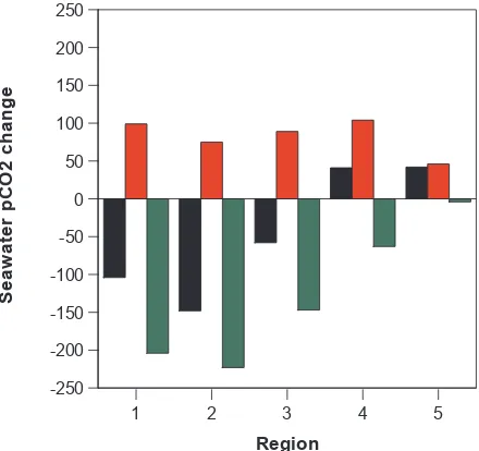
Fig. 10. Temperature and the “net biology” effects on seasonal change in calculated seawaterpCO₂( µatm) for the following re-gions of the Bering Sea shelf: (1) the North Line; (2) the Middle Line; (3) between Nunavak Island and Pribilof Islands, (4) south of the Probilof Islands, and; (5) SE Bering Sea shelf. In the bar chart, the black column denotes the mean observed change in seawater pCO2for each region (i.e.,δpCOspring

−summer

2 in Eq. 7), while the red and green columns indicates the changes imparted by temper-ature (δpCOtemperature₂ )and “net biology” (δpCObiology₂ ), respec-tively. 40 -250 -200 -150 -100 -50 0 50 100 150 200 250 S e a w a te r p C O 2 c h a n g e

1 2 3 4 5

Region

Figure 10. Temperature and the “net biology” effects on seasonal change in calculated seawater pCO2 (µatm) for the following regions of the Bering Sea shelf: (1) the North Line; (2) the Middle Line; (3) between Nunavak Island and Pribilof Islands, (4) south of the Probilof Islands, and; (5) SE Bering Sea shelf. In the bar chart, the black column denotes the mean observed change in seawater pCO2 for each region (i.e., δpCO2spring-summer in equation 7), while the red and green columns indicates the changes imparted by temperature

(δpCO2temperature) and “net biology” (δpCO2biology), respectively.

2370 2380 2390 2400 2410 2420 2430 2440 2450 Mean nTA+NO3

1 2 3 4 5

Region

Summer Spring

Figure 11. Spring to summer changes in observed surface nTA+NO3 (µmoles kg-1) for the following regions of the Bering Sea shelf: (1) the North Line; (2) the Middle Line; (3) between Nunavak Island and Pribilof Islands, (4) south of the Probilof Islands, and; (5) SE Bering Sea shelf.

4.1.1 Northern and central Bering Sea shelf

Over the northern and central Bering Sea shelf, there was a seasonal (i.e., spring to summer) drawdown of surface sea-water pCO2 of ∼100 µatm (Figs. 8 and 9). In the North Line, mean surface seawaterpCO2declined seasonally from 387.5±85.2 µ atm to 283.8±123.5 µatm. Similarly in the Middle Line and between Nunivak Island and the Pribilof Islands, mean surface seawater pCO2 declined seasonally from 367.4±56.2 µatm to 219.0±58.0 µatm, and 329.0± 35.9 µatm to 270.8±108 µatm, respectively. In comparison to seawaterpCO2changes, temperature corrected seawater pCO2 decreased seasonally by∼200 µatm (Figs. 8 and 9), and up to 300 µatm lower within the “green belt” area by the summertime. Thus, in these regions, the “net biology” effect strongly dominated the seasonal change in surface seawater pCO2compared to warming (Fig. 10). The 2008 BEST data indicates that the “net biology” effect seasonally decreases seawaterpCO2 by ∼150 to ∼230 µatm (Fig. 10) with this drawdown only partially compensated for by an increase in seawaterpCO2due to seasonal warming. For comparison, the Takahashi et al. (2002) climatology suggests that the sea-sonal drawdown of seawaterpCO2associated with “net bi-ology” effects is∼130–170 µatm. Furthermore, Mathis et al. (2010) show that large seasonal drawdown of DIC results from high rates of NCP particularly within the “green belt” area of the Bering Sea shelf. Analysis of seasonal changes in DIC, nitrate and silicate indicated mean Bering Sea shelf NCP rates that ranged from ∼20 to 55 mmoles C m−2_d−1 (Mathis et al., 2010, their Table 4). Within the “green belt” area, NCP rates computed from DIC changes ranged from 25 to 47 mmoles C m−2d−1(their Table 3). Given typical mixed layer depth of 30 m and growing season of 80–120 days, the above NCP rates would decrease seawaterpCO2by between ∼100 to ∼210 µatm similar to our values reported for the “net biology” effect. Our data provides further evidence that “net biology” (which is a near approximate of NCP) dom-inates the seasonal drawdown of seawater pCO2 for large areas of the Bering Sea shelf. Indeed, seasonal “net biology” effects or spring-summer NCP shifts much of the Bering Sea shelf from a neutral CO2 sink/source status in spring to a strong sink for CO2by summertime. The vertical export of organic carbon (as a result of high rates of NCP) and it’s rem-ineralization back to CO2in the subsurface appears to result in a buildup ofpCO2in the subsurface (Mathis et al., 2011). Late season mixing and water-column homogenization thus likely restores the Bering Sea shelf to near neutral CO2sink status in the fall before the wintertime return of sea-ice pro-vides a barrier to further CO2gas exchange.

4.1.2 Southern Bering Sea shelf

In contrast to the northern and central Bering Sea shelf, warming appears to dominate the seasonal changes of sea-water pCO2 for small areas south of the Pribilof Islands

and in the SE Bering Sea shelf region. In these two re-gions, mean surface seawater pCO2 increased seasonally from 297.1±33.0 µatm to 338.2±137.8 µatm, and from 293.0±55.2 µatm to 324.9±63.2 µatm, respectively. In these two regions, temperature corrected seawaterpCO2 de-creased seasonally by less than ∼50 µatm (Fig. 9). South of the Pribilof Islands, the seasonal “net biology” effect of ∼50 µatm was about half of the increase of seawaterpCO2 caused by warming (Fig. 10). In these regions, Mathis et al. (2010) compute relatively low rates of NCP of∼12 to 30 mmoles C m−2 d−1. In the SE Bering Sea shelf region, there was no seasonal “net biology” effect, and the increase in seawaterpCO2was due to warming only. Surface nitrate data in the SE Bering Sea shelf region were typically be-low 1 µmoles kg−1for both spring and summer cruises. This suggests that the typical “spring” phytoplankton bloom ob-served in the SE Bering Sea shelf had occurred earlier than the spring cruise, and that ocean biology had minimal im-pact on seawaterpCO2and air-sea CO2fluxes in the spring-summer period. This region also exhibits episodic coccol-ithophore blooms (e.g., Merico et al., 2004, 2006) that can increase seawaterpCO2(e.g., Bates et al., 1996b; Harley et al., 2010). Previous studies in the SE Bering Sea have shown some evidence for drawdown of alkalinity and increase in seawaterpCO2in late summer of 2000 in response to coc-colithophore blooms (Murata and Takizawa, 2002; Murata, 2006). However, there was no evidence in the BEST alka-linity (TA) or calculated seawaterpCO2data for significant impact of coccolithophore blooms in 2008. In all regions, there were no statistically significant changes in salinity nor-malized TA (i.e., here defined as nTA+NO3 to account for the contribution of nitrate to alkalinity; Brewer and Gold-man, 1978) from spring to summer (Fig. 11). nTA+NO3 were slighly lower south of the Pribilof Islands and in the SE Bering Sea shelf compared to other regions which sug-gests that if coccolithophores contributed significantly to the “spring” phytoplankton bloom, this occurred earlier than the spring cruise. In summary, in contrast to most of the Bering Sea shelf, seasonal warming shifted localized areas of the shelf from minor/neutral CO2 sink status to neutral/minor CO2source status.

4.2 2008 BEST data in context of seasonal changes in

seawaterpCO2and annual air-sea CO2fluxes

1248 N. R. Bates et al.: Air-sea CO2fluxes on the Bering Sea shelf

Figure 12

. Comparison of Takahashi

et al

. (2009) surface seawater

p

CO

and temperature

corrected seawater

p

CO

climatology for the Bering Sea shelf with observations from the

2008 BEST spring and summer cruises. The Takahashi

et al

. (2009) data have a spatial

resolution of 4° x 5° and monthly resolution. 2008 BEST spring and summer are binned and

averaged within each of four Takahashi

et al

. (2009) 4° x 5° that are defined for the Bering

Sea shelf. Please note that the mean values for observed data from the two 4° x 5° areas have

been slightly offset in time to allow for easier interpretation of data. (

a

) surface seawater

p

CO

for the 58°N-62°N/170°W-175°W (black symbols), and 58°N-62°N/175°W-180°W

(green symbols) areas. In each of the panels, Tahahashi

et al

. (2009) climatology data are

shown by open symbols while 2008 BEST spring and summer are shown as closed symbols

(mean and 1 std deviation); (

b

) surface temperature corrected seawater

p

CO

for the

58°N-62°N/170°W-175°W (black symbols), and 58°N-62°N/175°W-180°W (green symbols) areas;

(

c

) surface seawater

p

CO

for the 58°N/165°W-170°W (black symbols), and

54°N-58°N/170°W-175°W (green symbols) areas; and; (

d

) surface temperature corrected seawater

p

CO

for the 54°N-58°N/165°W-170°W (black symbols), and 54°N-58°N/170°W-175°W

(green symbols) areas. For the temperature corrected seawater

p

CO

datasets, both Takahashi

et al

. (2009) and 2008 BEST spring and summer data were corrected to 0°C using the

empirical relationships of Takahashi

et al

. (2002).

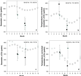
Fig. 12. Comparison of Takahashi et al. (2009) surface seawaterpCO₂and temperature corrected seawaterpCO₂climatology for the Bering Sea shelf with observations from the 2008 BEST spring and summer cruises. The Takahashi et al. (2009) data have a spatial resolution of 4◦×5◦and monthly resolution. 2008 BEST spring and summer are binned and averaged within each of four Takahashi et al. (2009) 4◦×5◦ that are defined for the Bering Sea shelf. Please note that the mean values for observed data from the two 4◦×5◦areas have been slightly offset in time to allow for easier interpretation of data. (a) surface seawaterpCO2for the 58◦N–62◦N/170◦W–175◦W (black symbols), and 58◦N–62◦N/175◦W–180◦W (green symbols) areas. In each of the panels, Tahahashi et al. (2009) climatology data are shown by open symbols while 2008 BEST spring and summer are shown as closed symbols (mean and 1 std deviation); (b) surface temperature corrected seawaterpCO₂for the 58◦N–62◦N/170◦W–175◦W (black symbols), and 58◦N–62◦N/175◦W–180◦W (green symbols) areas; (c) surface seawaterpCO2for the 54◦N–58◦N/165◦W–170◦W (black symbols), and 54◦N–58◦N/170◦W–175◦W (green symbols) areas; and; (d) surface temperature corrected seawaterpCO₂for the 54◦N–58◦N/165◦W–170◦W (black symbols), and 54◦N–58◦N/170◦W–175◦W (green symbols) areas. For the temperature corrected seawaterpCO2datasets, both Takahashi et al. (2009) and 2008 BEST spring and summer data were corrected to 0◦C using the empirical relationships of Takahashi et al. (2002).

drawdown (Fig. 12) that causes the shelf to act as a CO2sink (∼1–2 mol C m−2yr−1). However, an important caveat is that the seawaterpCO2climatology is based on very limited data (1 cruise), and thus it is difficult to draw firm conclu-sions about the seasonal and annual CO2sink-source status of the Bering Sea shelf.

The Takahashi et al. (2009) seawater pCO2 climatology has four 4◦×5◦ areas that overlie the Bering Sea shelf (Fig. 12). For July, average1pCO2values range from−20.8 to−44.7 µatm for these four. In contrast, the 2008 BEST summer mean1pCO2values ranged from −110.8 µatm to −170.4 µatm for the same areas, indicating that the shelf was much more strongly undersaturated than the seawaterpCO2 climatology suggests. As a consequence, the mean July

air-to-sea CO2fluxes calculated here were about 5 times higher (∼ −16.3 to−24.2 mmoles m−2d−1)than the Takahashi et al. (2009) seawaterpCO2climatology.

Table 1. Estimates of the annual air-sea CO2flux on the Bering Sea shelf, assuming 500,000 km2of shelf area, and 180 days of open water.

Study daily flux annual flux Bering Sea annual flux flux

(mmoles CO₂m−2d−1) (moles CO₂m−2yr−1) (Tg C yr−1)

Walsh and Dieterle (1994) n/a 4.3 3.4

Chen and Borges −1.2aand 0.66b n/a 11

Tahahashi et al. (2009) 2 n/a 37

This study 22±3 n/a 157±35

Chen et al. (2004) n/a n/a 200

a_{Nedashkovskii and Sapozhnikov (2001);}b_{Codispoti et al. (1986)}

recently, Chen and Borges (2009) summarized coastal air-sea CO2fluxes, reporting springtime and summertime fluxes of ∼ −1.2 mmol C m−2d−1 (Nedashkovskii and Sapozhnikov, 2001) and 0.66 mmol C m−2d−1(Codispoti et al., 1986), re-spectively. If we scale up these flux rates, accounting for Bering Sea surface area and period of open water conditions, we estimate a net annual CO2sink of∼11 Tg C yr−1. Sim-ilarly, scaling our observations and the climatology of Taka-hashi et al. (2009), we compute that the Bering Sea shelf CO2 sink was 157±35 Tg C yr−1 and ∼37 Tg C yr−1, re-spectively (Table 1). The primary difference between the 2008 BEST datasets and Takahashi et al. (2009) seawater pCO2 climatology relates to the much larger undersatura-tion observed in surface waters during summertime in 2008 (Fig. 12). Our annual estimate of 157±Tg C yr−1, compares to the estimates for the entire Bering Sea of 200 Tg C yr−1 previously reported by Chen et al. (2004). In compari-son, annual rates of NCP or PP have been estimated at 99±29 Tg C yr−1(Mathis et al., 2010) and 102 Tg C yr−1, respectively (Springer, 1986). Thus the gas exchange term appears to be∼50 % higher than the NCP term, at least for 2008.

There are many caveats in scaling any of the above flux data to annual CO2 flux rates and caution must be consid-ered in undertaking this scaling up and interpreting such re-sults. If the 2008 BEST datasets are indeed representative of typical conditions, then the Bering Sea shelf is a much larger CO2sink than previously thought. At the very least, such uncertainties in providing an accurate assessment of the annual CO2 sink-source status of the Bering Sea shelf, re-quires future long-term monitoring efforts for this important shelf region. It should also be noted that an extensive coc-colithophore bloom was not observed in the Bering Sea in 2008, but this phenomena has been observed in prior years (e.g., Murata and Takizawa, 2002; Murata, 2006; Merico et al., 2004, 2006) and in 2009. Since coccolithophore calcifi-cation can result in an increase of seawaterpCO2(e.g., Bates et al., 1996b; Harley et al., 2010), the Bering Sea shelf CO2 sink may be much reduced in those years with significant coccolithophore bloom events, for example, in 2000 (Mu-rata, 2006).

5 Conclusions

1250 N. R. Bates et al.: Air-sea CO2fluxes on the Bering Sea shelf

Acknowledgements. The authors wish to thank the officers and

crew of the USCGC Healy for their logisitical support as well as our collegues in the BEST-BSIERP project for allowing us to make these measurements. We would like to specifically thank the hydrographic team at NOAA-PMEL including Phyllis Stabeno, Calvin Moordy, Nancy Kachel, and many others who helped in sample collection and provided high quality temperature, salinity, oxygen and nutrient data. The work presented in this paper was supported by the Bureau of Ocean Energy Management, Regulation and Enforcement and the Coastal Marine Institute at the University of Alaska Fairbanks under Agreement M08AC12645.

Edited by: M. Dai

References

Antonov, J. I., Locarnini, R. A., Boyer, T. P., Mishonov, A. V., and Garcia, H. E.: World Ocean Atlas 2005, Volume 2: Salinity, edited by: Levitus, S., NOAA Atlas NESDIS 62, US Govern-ment Printing Office, Washington, DC, 182 pp., 2006.

Banse, K. and English, D. C.: Comparing phytoplankton seasonal-ity in the Eastern and Western subarctic Pacific and the Western Bering Sea, Prog. Oceanogr., 43, 235–288, 1999.

Bates, N. R.: Air-sea CO2fluxes and the continental shelf pump of carbon in the Chukchi Sea adjacent to the Arctic Ocean, J. Geo-phys. Res.-Oceans, 111, C10013, doi:10.129/2005JC003083, 12 October 2006.

Bates, N. R. and Mathis, J. T.: The Arctic Ocean marine carbon cycle: evaluation of air-sea CO2exchanges, ocean acidification impacts and potential feedbacks, Biogeosciences, 6, 2433–2459, doi:10.5194/bg-6-2433-2009, 2009.

Bates, N. R., Michaels, A. F., and Knap, A. H.: Seasonal and inter-annual variability of the oceanic carbon dioxide system at the US JGOFS Bermuda Atlantic Time-series Site, Deep-Sea Res. Pt. II, 43(2–3), 347–383, doi:10.1016/0967-0645(95)00093-3, 1996a. Bates, N. R., Michaels, A. F., and Knap, A. H.: Alkalinity changes

in the Sargasso Sea: Geochemical evidence of calcification?, Mar. Chem., 51(4), 347–358, doi:10.1016/0304-4203(95)00068-2, 1996b.

Bates, N. R., Pequignet, A. C., and Sabine, C. L.: Ocean car-bon cycling in the Indian Ocean: II. Estimates of net com-munity production, Global Biogeochem. Cy., 20(3), GB3021, doi:10.1029/2005GB002492, 2006b.

Bates, N. R., Pequignet, A. C., and Sabine, C. L.: Ocean carbon cy-cling in the Indian Ocean: 1. Spatiotemporal variability of inor-ganic carbon and air-sea CO2gas exchange, Global Biogeochem. Cy., 20(3), GB3020, doi:10.1029/2005GB002491, 2006a. Bond, N. A., Overland, J. E., Spillane, M., and Stabeno, P.:

Re-cent shifts in the state of the North Pacific, Geophys. Res. Lett., 30(23), 2183, doi:10.1029/2003GL018597, 2003.

Bond, N. A. and Overland, J. E.: The importance of episodic weather events to the ecosystem of the Bering Sea shelf, Fish. Oceanogr., 14(2), 97–111, 2005.

Brewer, P. G. and Goldman, J. C.: Alkalinity changes generated by phytoplankton growth, Limnol. Oceanogr., 21(1), 108–117, 1976.

Broerse, A. T. C., Tyrell, T., Young, J. R., Poulton, A. J., Merico, A., Balch, W. M., and Miller, P. I.: The cause of bright waters in the Bering Sea in winter, Cont. Shelf Res., 23, 1579–1596, 2003.

Chen, C. T.-A.: Carbonate chemisrty of the wintertime Bering Sea marginal ice zone, Cont. Shelf Res., 13(1), 67–87, 1993. Chen, C. T. A. and Borges, A. V.: Reconciling opposing

views on carbon cycling in the coastal ocean: continental shelves as sinks and near-shore ecosystems as sources of at-mospheric CO2, Deep-Sea Res. Pt. II, 56(8–10), 578–581, doi:10.1016/j.dsr2.2009.01.001, 2009.

Chen, C. T.-A., Andreev, A., Kim, K. R., and Yamamoto, M.: Roles of continental shelves and marginal seas in the biogeochemical cycles of the North Pacific Ocean, J. Oceanogr., 60(1), 17–44, 2004.

Chen, L. and Gao, Z.: Spatial variability in the partial pressures of CO2in the Northern Bering and Chukchi seas, Deep-Sea Res. Pt. II, 54, 2619–2629, 2007.

Coachman, L. K.: Circulation, water masses, and fluxes on the southeastern Bering Sea shelf, Cont. Shelf Res., 5, 23–108, 1986. Coatanoan, C., Goyet, C., Gruber, N., Sabine, C. L., and Warner, M.: Comparison of two approaches to quantify anthro-pogenic CO₂ in the ocean: results from the northern Indian Ocean, Global Biogeochem. Cy., 15, 11–25, 2001.

Codispoti, L. A., Friederich, G. E., Iverson, R. L., and Hood, D. W.: Temporal changes in the inorganic carbon system of the South-eastern Bering Sea during spring 1980, Nature, 296, 242–245, 1982.

Codispoti, L. A., Friederich, G. E., and Hood, D. W.: Variability in the inorganic carbon system over the Southeastern Bering Sea shelf during spring 1980 and spring-summer 1981, Cont. Shelf Res., 5, 133–160, 1986.

Comiso, J. C., Parkinson, C. L., Gersten, R., and Stock, L.: Accel-erated decline in the Arctic sea ice cover, Geophys. Res. Lett., 35, L01703, doi:10.1029/2007GL031972, 2008.

Delille, B., Jourdain, B., Borges, A. V., Tison, J.-L., and Delille, D.: Biogas (CO2, O2, dimethylsulfide) dynamics in spring Antarctic fast ice, Limnol. Oceanogr., 52, 1367–1379, 2007.

Dickson, A. G. and Millero, F. J.: A comparison of the equilibrium constants for the dissociation of carbonic acid in seawater media, Deep-Sea Res., 34, 1733–1743, 1987.

Dickson, A. G., Sabine, C. L., and Christian, J. R.: Guide to best practices for ocean CO2 measurements, Sidney, British Columbia, North Pacific Marine Science Organization, PICES Special Publication 3, 2007.

Ducklow, H. W. and McAllister, S. L.: Biogeochemistry of car-bon dioxide in the coastal oceans, in: The Sea, Volume 13, The Global Coastal Ocean-Multiscale Interdisciplinary Processes, edited by: Robinson, A. R. and Brink, K., J. Wiley and Sons, NY, 2005.

Garcia, H. E., Locarnini, R. A., Boyer, T. P., and Antonov, J. I.: World Ocean Atlas 2005, Volume 3: Dissolved Oxygen, Appar-ent Oxygen Utilization, and Oxygen Saturation, edited by: Lev-itus, S., NOAA Atlas NESDIS 63, US Government Printing Of-fice, Washington, DC, 342 pp., 2006a.

Garcia, H. E., Locarnini, R. A., Boyer, T. P., and Antonov, J. I.: World Ocean Atlas 2005, Volume 4: Nutrients (phosphate, ni-trate, silicate), edited by: Levitus, S., NOAA Atlas NESDIS 64, US Government Printing Office, Washington, DC, 396 pp., 2006b.

ftp.cmdl.noaa.gov, Path: ccg/co2/GLOBALVIEW, 2007. Gosink, T. A., Pearson, J. G., and Kelley, J. J.: Gas movement

through sea ice, Nature, 263, 41–42, doi:10.1038/263041al, 1976.

Goyet, C. and Poisson, A. P.: New determination of carbonic acid dissociation constants in seawater as a function of temperature and salinity, Deep-Sea Res., 36, 1635–1654, 1989.

Goyet, C. and Davis, D.: Estimation of total CO2 concentration throughout the water column, Limnol. Oceanogr., 44, 859–877, 1997.

Grebmeier, J. M., Cooper, L. W., Feder, H. M., and Sirenko, B. I.: Ecosystem dynamics of the Pacific-influenced Northern Bering and Chukchi Seas in the Amerasian Arctic, Prog. Oceanogr., 71(2–4), 331–361, 2006a.

Grebmeier, J. M., Overland, J. E., Moore, S. E., Farley, E. V., Car-mack, E. C., Cooper, L. W., Frey, K. E., Helle, J. H., McLaugh-lin, F. A., and McNutt, S. L.: A major ecosystem shift in the Northern Bering Sea, Science, 311(5766), 1461–1464, 2006b. Grebmeier, J. M., Bates, N. R., and Devol, A.: Continental Margins

of the Arctic Ocean and Bering Sea, in: North American Con-tinental Margins: A Synthesis and Planning Workshop, edited by: Hales, B., Cai, W.-J., Mitchell, B. G., Sabine, C. L., and Schofield, O., 120 pp., 61–72, 2008.

Hansell, D. A., Goering, J. J., Walsh, J. J., McRoy, C. P., Coach-man, L. K., and Whitledge, T. E.: Summer phytoplankton pro-duction and transport along the shelf break front in the Bering Sea, Cont. Shelf Res., 9, 1085–1104, 1989.

Harley, J., Borges, A. V., Van Der Zee, C., Delille, B., Godi, R. H. M., Schiettecatte, L.-S., Roevros, N., Aerts, K., Plapernat, P.-E., Rebreanu, L., Groom, S., Daro, M.-H., Van Grieken, R., and Chou, L.: Biogeochemical study of coc-colithophore bloom in the northern Bay of Biscay (NE At-lantic Ocean) in June 2004, Prog. Occeanogr., 86, 317–336, doi:10.1016/j.pocean.23010.04.029, 2010.

Hollowed, A. B., Hare, S. R., and Wooster, W. S.: Pacific Basin climate variability and patterns of Northeast Pacific marine fish populations, Prog. Oceanogr., 49, 257–282, 2001.

Hunt, G. L., Stabeno, P., Walters, G., Sinclair, E., Brodeur, R. D., Napp, J. M., and Bond, N. A.: Climate change and control of the Southeastern Bering Sea pelagic ecosystem, Deep-Sea Res. Pt. II, 49(26), 5821–5853, 2002.

Kelley, J. J. and Hood, D. W.: Carbon dioxide in the surface water of the ice-covered Bering Sea, Nature, 229, 37–39, 1971. Key, R. M., Kozyr, A., Sabine, C. L., Lee, K., Wanninkhof, R.,

Bullister, J. L., Feely, R. A., Millero, F. J., Mordy, C., and Peng, T.-H.: A global ocean carbon climatology: results from Global Data Analysis Project (GLODAP), Global Biogeochem. Cy., 18, GB4031, doi:10.1029/2004GB002247, 2004.

Lee, K.: Global net community production estimated from the an-nual cycle of surface water total dissolved inorganic carbon, Lim-nol. Oceanogr., 46(6), 1287–1297, 2001.

Lee, K., Karl, D. M., Wanninkhof, R., and Zhang, J. Z.: Global estimates of net carbon production in the nitrate-depleted tropical and subtropical oceans, Geophys. Res. Lett., 29(19), 1907, 2002. Locarnini, R. A., Mishonov, A. V., Antonov, J. I., Boyer, T. P., and Garcia, H. E.: World Ocean Atlas 2005, Volume 1: Temperature, edited by: Levitus, S., NOAA Atlas NESDIS 61, US Govern-ment Printing Office, Washington, DC, 182 pp., 2006.

Macklin, S. A., Hunt, G. L., and Overland, J. E.: Collaborative

re-search on the pelagic ecosystem of the Southeastern Bering Sea shelf, Deep-Sea Res. Pt. II, 49(26), 5813–5819, 2002.

Mathis, J. T., Cross, J. N., Bates, N. R., Bradley Moran, S., Lo-mas, M. W., Mordy, C. W., and Stabeno, P. J.: Seasonal dis-tribution of dissolved inorganic carbon and net community pro-duction on the Bering Sea shelf, Biogeosciences, 7, 1769–1787, doi:10.5194/bg-7-1769-2010, 2010.

Mathis, J. T., Cross, J., and Bates, N. R.: Coupling primary pro-duction and terrestrial runoff to ocean acidification and carbon-ate mineral suppression in the eastern Bering Sea, Global Bio-geochem. Cy., 116, C02030, doi:10.1029/2010JC006453, 2011. McRoy, C. P. and Goering, J. J.: The influence of ice on the

pri-mary productivity of the Bering Sea, in: Oceanography of the Bering Sea with Emphasis on Renewable Resources, edited by: Hood, D. W. and Kelley, E. J., Univ. of Alaska, Fairbanks, 403– 421, 1974.

Mehrbach, C., Culberson, C. H., Hawley, J. E., and Pytkow-icz, R. M.: Measurement of the apparent dissociation constants of carbonic acid in seawater at atmospheric pressure, Limnol. Oceanogr., 18, 897–907, 1973.

Merico, A., Tyrrell, T., Lessard, E. J., Oguz, T., Stabeno, P. J., Zee-man, S. I., and Whitledge, T. E.: Modelling phytoplankton suc-cession on the Bering Sea role of climate influences and trophic interactions in generating Emiliania huxleyi blooms 1997–2000, Deep-Sea Res. Pt. I, 51(12), 1803–1826, 2004.

Merico, A., Tyrrell, T., and Cokacar, T.: Is there any relationship be-tween phytoplankton seasonal dynamics and the carbonate sys-tem? J. Marine Syst., 59(1–2), 120–142, 2006.

Midorikawa, T., Umeda, T., Hiraishi, N., Ogawa, K., Nemoto, K., Kubo, N., and Ishii, M.: Estimation of seasonal net commu-nity production and air-sea CO2flux based on the carbon budget above the temperature minimum layer in the Western subarctic North Pacific, Deep-Sea Res. Pt. I, 49(2), 339–362, 2002. Miller, L. A., Papakyriakou, T. N., Collins, R. E., Deming, J.

W., Ehn, J., Macdonald, R. W., Mucci, A., Owens, O., Raud-sepp, M., and Sutherland, N.: Carbon dynamics in Sea Ice: A Winter Flux Time Series, J. Geophys. Res., 116, C02028, doi:0.1029/2009JC006058, 2011.

Millero, F. J., Graham, T. B., Huang, F., Bustos-Serrano, H., and Pierrot, D.: Dissociation constants of carbonic acid in seawater as a function of salinity and temperature, Mar. Chem., 100, 80– 94, 2006.

Murata, A. and Takizawa, T.: Impact of a coccolithophorid bloom on the CO₂system in surface waters of the Eastern Bering Sea shelf, Geophys. Res. Lett., 29(11), 1547, 2002.

Murata, A.: Increased surface seawater pCO2 in the east-ern Bering Sea shelf: an effect of blooms of coc-colithophorid Emiliania huxleyi?, Global Biogeochem. Cy., GB4006, doi:10.1029/2005GB002615, 2006.

Murphy, P. P., Nojiri, Y., Harrison, D. E., and Larkin, N. K.: Scales of spatial variability for surface ocean pCO₂ in the Gulf of Alaska and Bering Sea: toward a sampling strategy, Geophys. Res. Lett., 28(6), 1047–1050, 2001.

Nagurnyi, A. P.: On the role of Arctic sea-ice in seasonal variabil-ity of carbon dioxide concentration in Northern Latitudes, Russ. Meteor. Hydrol., 33(1), 43–47, 2008.