Quantifying wetland methane emissions with process-based models of different complexities

www.biogeosciences.net/7/3817/2010/ doi:10.5194/bg-7-3817-2010

© Author(s) 2010. CC Attribution 3.0 License.

Biogeosciences

Quantifying wetland methane emissions with process-based models

of different complexities

J. Tang1,2, Q. Zhuang1,2,3, R. D. Shannon4, and J. R. White5

1_{Dept. of Earth and Atmospheric Sciences, Purdue University, West Lafayette, Indiana, USA} 2_{Purdue Climate Change Research Center, West Lafayette, Indiana, USA}

3_{Department of Agronomy, Purdue University, West Lafayette, Indiana, USA}

4_{Department of Agricultural & Biological Engineering, Pennsylvania State University, University Park, Pennsylvania, USA} 5_{Biogeochemical Laboratories & Center for Research in Environmental Sciences, Indiana Univ., Bloomington, Indiana, USA}

Received: 2 July 2010 – Published in Biogeosciences Discuss.: 16 August 2010

Revised: 10 November 2010 – Accepted: 13 November 2010 – Published: 25 November 2010

Abstract. Bubbling is an important pathway of methane emissions from wetland ecosystems. However the concentration-based threshold function approach in current biogeochemistry models of methane is not sufficient to rep-resent the complex ebullition process. Here we revise an extant process-based biogeochemistry model, the Terrestrial Ecosystem Model into a multi-substance model (CH4, O2,

CO2and N2) to simulate methane production, oxidation, and

transport (particularly ebullition) with different model com-plexities. When ebullition is modeled with a concentration-based threshold function and if the inhibition effect of oxy-gen on methane production and the competition for oxyoxy-gen between methanotrophy and heterotrophic respiration are re-tained, the model becomes a two-substance system. Ignor-ing the role of oxygen, while still modelIgnor-ing ebullition with a concentration-based threshold function, reduces the model to a one-substance system. These models were tested through a group of sensitivity analyses using data from two temper-ate peatland sites in Michigan. We demonstrtemper-ate that only the four-substance model with a pressure-based ebullition al-gorithm is able to capture the episodic emissions induced by a sudden decrease in atmospheric pressure or by a sud-den drop in water table. All models captured the retardation effect on methane efflux from an increase in surface stand-ing water which results from the inhibition of diffusion and the increase in rhizospheric oxidation. We conclude that to

Correspondence to: J. Tang ([email protected])

more accurately account for the effects of atmospheric pres-sure dynamics and standing water on methane effluxes, the multi-substance model with a pressure-based ebullition algo-rithm should be used in the future to quantify global wetland CH4emissions. Further, to more accurately simulate the pore

water gas concentrations and different pathways of methane transport, an exponential root distribution function should be used and the phase-related parameters should be treated as temperature dependent.

1 Introduction

Methane (CH4) emitted from natural wetlandsis a

signifi-cant component of its atmospheric budget. Biogeochemistry and atmospheric inversion models estimate the total wet-land emissions to be 100–230 Tg CH4y−1, around 25% of

the global emissions into the atmosphere under the current climate condition (Denman et al., 2007). Inverse modeling estimates the strengths of various CH4 sources and sinks

by comparing the model simulated CH4 concentrations to

spatially discrete and temporally continuous observations of the atmospheric CH4concentrations (e.g. Houweling et al.,

1999). Since all sources/sinks are treated simultaneously in the inversion, the total CH4 emissions into the atmosphere

can be well constrained. However, there are various limi-tations including the sparse in-situ observation networks of atmospheric CH4and unclear sources and sinks due to

modeling are usually subject to great uncertainties. Process-based models integrate and extrapolate the knowledge from field studies at limited sites to regional and global scales. Be-cause of sparse site-level information and inadequate repre-sentation of CH4 processes in these models, the

uncertain-ties in the quantification from biogeochemical modeling are also substantial (e.g., Walter et al., 2001; Zhuang et al., 2004, 2009; Denman et al., 2007).

To date, a group of process-based models with different complexities have been developed to quantify the spatial and temporal patterns of wetland CH4emissions. Among them,

the one-substance models are widely used (e.g., Walter and Heimann, 2000; Zhuang et al., 2004; van Huissteden et al., 2006). These models focus on CH4 only, and assume that

methanogenesis and methanotrophy occur in anoxic and oxic zones, respectively, which are spatially separated by the po-sition of water table. In contrast, the two-substance model considers CH4and O2simultaneously, and the

methanogen-esis and methanotrophy occur according to the status of both gases in soils (e.g., Arah and Kirk, 2000). This is accom-plished by introducing the inhibition effect of O2 on CH4

production and the competition for O2between heterotrophic

respiration and methanotrophy. As such, CH4oxidation and

heterotrophic respiration dominate in the oxic zone while CH4 production dominates in the anoxic zone. The

two-substance models have been used in modeling CH4

emis-sions from rice paddies (Matthews et al., 2000), and showed reasonable results compared with field measurements. Other existing models are conceptually of either one-substance or two-substance model structure (e.g., Potter, 1997; Zhang et al., 2002).

In biogeochemistry models, three pathways for gas trans-port are considered: (1) molecular diffusion, (2) plant-aided transport and (3) ebullition, though some models lump the three pathways together (e.g., Cao et al., 1995; Sass et al., 2000; Zhang et al., 2002). Ebullition, if considered explic-itly, is often modeled as a threshold phenomenon using the Heaviside function with some universally prescribed thresh-old concentration of the dissolved gases (e.g., Walter and Heimann, 2000; Matthews et al., 2000). Field and analytical studies suggest such a simple algorithm does not fully repre-sent the physical processes of ebullition (Bazhin, 2001, 2004; Baird et al., 2004; Tokida et al., 2005, 2007). Specifically, several factors have not been considered in the concentration-based threshold function algorithms: (1) the composition of the bubbles affected by multiple substances such as CO2and

N2; (2) the effects of the hydrostacy affected by water table

dynamics and atmospheric pressure variation (Bazhin, 2001; Tokida et al., 2005, 2007) and (3) the ebullition threshold de-fined in terms of gas volumes is fuzzy rather than determin-istically predictable because of possible re-dissolution and gas entrapping, during the course of ebullition (Martens and Klump, 1980; Kellner et al., 2006; Coulthard et al., 2009).

In this study, we revise the CH4 module in a

biogeo-chemistry model, the Terrestrial Ecosystem Model (TEM)

(Zhuang et al., 2004) by incorporating the effects of multi-ple substances in a soil profile and a probabilistic pressure-based algorithm for ebullition. We apply the revised model to two temperate peatland ecosystems to demonstrate the im-portance of considering the effects of multiple substances in soils on episodic emissions during atmospheric pressure changes (Mattson and Likens, 1990). We also demonstrate the retardation effects of increases in standing water depth on CH4effluxes when different model complexities are

as-sumed (Jauhiainen et al., 2005; Zona et al., 2009).

2 Methods

2.1 Overview

We developed a four-substance CH4module within a

biogeo-chemistry model, the Terrestrial Ecosystem Model (Zhuang et al., 2004). The model was calibrated and applied to data from two temperate peatland sites in Michigan to demon-strate the capabilities of models with different complexities in simulating CH4effluxes. A group of sensitivity analyses

were conducted to assess the need for a four-substance model with an improved ebullition algorithm.

2.2 The revised CH4module

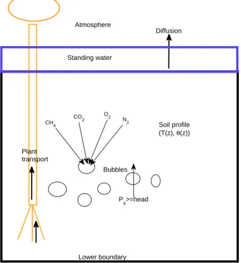
The governing equation for a non-adsorbed substrate in a soil column (Fig. 1) is:

∂y

∂t =

∂ ∂z

D∂y

∂z

+P −Q−E −R

min(0,zwt)≤z≤Zsoil (1)

where

∂ ∂z

D∂y_∂z:Diffusion

P: Production

Q: Consumption

E: Ebullition

R: Plant transport

(2)

andzwt (unit: m) is the water table depth, being negative

when it is above the soil surface. For substance i, the bulk concentration yi (unit: mol m−3) is related to its aqueous

concentrationyi,w (unit: mol m−3 water) and gaseous

con-centrationyi,a(unit: mol m−3air) through

yi =yi,a +θyi,w = ( +θ αi)yi,a (3)

where(z,t )(unit: m3air m−3soil) is air-filled porosity, αi

is the Bunsen coefficient for gas i (see Appendix A for its calculation) andθ (z,t )(unit: m3water m−3soil) is the vol-umetric soil moisture.

The boundary conditions for Eq. (1) are

Bubbles

N₂ O₂ CO₂ CH

4

Lower boundary

Soil profile (T(z), θ(z)) Atmosphere

Standing water

Diffusion

P

s>=head

Plant transport

Fig. 1. Diagram showing the three major gas-transport pathways involved in the multi-substance CH₄ model. See text for details about the calculations.

∂y

∂z = 0 for nonvolatiles (5)

at the upper boundary (z=min(0,zwt)) and

∂y

∂z = 0 (6)

at the lower boundary (z=Zsoil) for all substrates.

2.2.1 Chemistry involved in methane production and consumption

In wetland ecosystems, CH4 is produced primarily through

methanogenesis

CH2O+CH2O → CO2 +CH4 (7)

and consumed through methanotrophy

CH4 +2O2 → CO2 +2H2O (8)

Methanogenesis can proceed in either of the two path-ways (Conrad, 1989), i.e. CO2+4H2→CH4+2H2O, or

CH3COO−+H+→CO2+CH4, both of which can

equiva-lently be reduced to Eq. (7). Though there are other path-ways, e.g. HCOO−₊1

2H2O+ 1 4CO2→

1

4CH4+HCO − 3, and

CH3OH→ 3₄CH4+1₂H2O+1₄CO2, leading to CH4

produc-tion, we assumed they are minor as indicated in previous studies (Conrad, 1989). If one makes the assumption that

dissolved oxygen is negligible in the aqueous phase, then the water table serves as a boundary in the soil between the oxic zone above the water table and the anoxic zone below the water table. Consequently, the equation to solve for the wetland CH4 profile in a soil column is reduced to a

sys-tem of a single substance, i.e. CH4, only. Such was adopted

in Walter et al. (2001) and Zhuang et al. (2004), where the bubbling was modeled as a switch-on and -off process with a prescribed threshold CH4 concentration, CH4,max (unit:

mol m−3water).

If one considers the competition for O2in CH4oxidation

and respiration processes, a third stoichiometry is involved:

CH2O+O2 → CO2 +H2O (9)

With such, we obtained a two-substance model considering both CH4and O2in a soil profile. Characterization of the

aer-obic and anaeraer-obic zone in a soil column by the water table in the one-substance system is now revised by introducing the inhibition of O2on CH4production

PCH4 = P

∗

CH4/(1 +ηyO2,w) (10)

where P_CH∗

4 (unit: mol m

−3_s−1_{) is the maximum CH} 4

production potential when the environment is completely anoxic, andη(unit: m3 water mol−1_{) is a parameter}

repre-senting the sensitivity of methanogenesis to the concentra-tion of dissolved oxygen yO2,w in pore water. A value of

400 m3 water mol−1 from Arah and Kirk (2000) was used forη.P_CH∗

4is defined in Appendix B.

Accordingly, the methanotrophy is restricted by the avail-ability of O2as

QCH4 =Q

∗ CH4

yCH4,w

kCH4 +yCH4,w

yO2,w

kO2 +yO2,w

(11) whereQ∗_CH

4 (unit: mol m

−3_s−1_{) is the oxidation potential}

when aqueous O2 and CH4 are not limited, and kCH4 and

kO2 are Michaelis-Menten constants (unit: mol m

−3_water)

for CH4and O2. We use values of 0.44 mol m−3water and

0.33 mol m−3water, respectively, forkCH4andkO2(Arah and

Kirk, 2000).Q∗_CH

4 is defined in Appendix B.

The consumption of O2 due to heterotrophic respiration

and CH4oxidation is modeled as

QO2 = 2QCH4 +V

∗ R

yO2,w

kR +yO2,w

(12) whereV_R∗ is the maximum rate of respiration when O2 is

not the limiting factor,kRis the Michaelis-Menten constant,

using a value of 0.22 mol m−3water (Arah and Kirk, 2000). As in Matthews et al. (2000), we assumed only the pro-cess of heterotrophic respiration competes with the propro-cess of methanotrophy for O2, thusVR∗is twice that ofP

∗ CH4. We

also neglected the O2consumption by electron acceptor

re-oxidation (Segers and Leffelaar, 2001; van Bodegom et al., 2001) for the moment. Since no O2is produced in the soil,

(1) Initialize the total bubble flux E to zero (2) DO I = N, N0, −1

(3) Compute potential bubble flux Eb at layer l IF Eb <= 0 .AND. E = 0 THEN

GOTO step(2) ELSE

IF Eb >= 0 THEN

(4) Combine the bubbles, E=E+Eb ELSE

(5) Draw a random number u from uniform distribution U[0,1] IF u <= abs(Eb)/(abs(Eb)+E) THEN

IF abs(Eb) <= E THEN

(6) Dissolve bubbles to make equality in Eq.(14) hold at layer l, and update, E=E−abs(Eb)

ELSE

(7) Dissolve bubbles with the amount E, thus E=0 ENDIF

ENDIF ENDIF ENDIF ENDDO

(8) Release E to the atmosphere or add directly to the soil layer that is right above the water table.

Here, N is node ID of the bottom layer of the computation grids, and N0 is node ID of the water table.

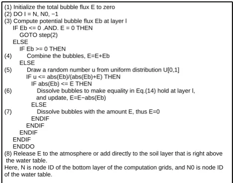
Fig. 2. The probabilistic algorithm used in the S4 model to compute ebullition.

Carbon dioxide is produced in methanogenesis, methan-otrophy and aerobic respiration:

PCO2 = PCH4 +QO2 −QCH4 (13)

Just as for O2consumption, CO2production from electron

acceptor reduction (Conrad, 1989) was also neglected here. In the soil, consumption of CO2is zero, therefore,QCO2=0.

For N2, we assumed no production and consumption in the

soil profile, therefore,PN2=QN2=0.

2.2.2 The pressure-based ebullition algorithm

We revised TEM to consider effects of hydrostacy on ebulli-tion. Tokida et al. (2007) observed an abrupt change in the CH4emission rates associated with a decreasing atmospheric

pressure, and the mixing ratio of CH4in the gas bubbles was

no more than 50% (see their Fig. 2). Zona et al. (2009) found that, when the surface standing water increased, the CH4

ef-flux was effectively retarded. Such behavior has not been explicitly considered and modeled in the process-based CH4

models with the conventional algorithms of ebullition using a prescribed threshold of water dissolved CH4 (e.g.,

Wal-ter and Heimann, 2000; Arah and Kirk, 2000; Zhuang et al., 2004). Tokida et al. (2007) suggested a three-substance sys-tem, including CH4, CO2and N2, should be used to model

the ebullition. Indeed, Bazhin (2001, 2004) suggested that ebullition is triggered at a certain depth when the total pres-sure of the water-dissolved gases exceeds the hydrostatic pressure imposed at that depth by the water table and at-mospheric pressure. Therefore, the simple concentration-based threshold approach was replaced by an equation of hydrostatic equilibrium. In this study, we considered a four-substance system, i.e. CH4, O2, CO2 and N2, and ignored

other possible trace gases (e.g. argon and hydrogen). We for-mulated the bubbling criterion (Fig. 1) as

Ps= X

i Psi=

X

i

yi,w(z)

Hi(z)

≥P0

ˆ

p+ b

z0

+zd

z0

=head (14)

wherePsiis the partial pressure andHi(see Appendix A for

the formula) is the Henry’s law constant for gas i,pˆ(=p/P0)

is the scaled atmospheric pressure,P0=105Pa, z0=10 m,

andzd=min(z−zs,z−zwt), and

b =

(_z

s −zwt, ifzwt < 0 Rzwt

zs

θ (z)

θs(z)dz,ifzwt ≥ 0

(15)

wherezs is the depth of soil surface, set to 0.0; and head

(unit: Pa) is the total hydrostatic pressure head imposed by atmosphere and water above depthz. The second equation in Eq. (15) accounts for the capillary force by considering the rate of saturation of the soil. Further we assumed bubbling only occurs below the water table, thus zd is always

non-negative. Note, in Eq. (14), we did not consider the effects of bubble shapes and number of bubbles, which would impact the surface tension between the bubble and water interface and consequently the bubbling criterion (Peck, 1960). We also neglected the change of water distribution caused by the ebullition (Rosenberry et al., 2003), which would cause some bubbles to be trapped and released later.

With Eq. (14), the potential ebullition for gas i at a certain depthzis computed as

Ebi =

Z Zsoil

zwt

(yi(s) − ˜yi(s))δ(s −z)ds (16)

where the equilibrium bulk concentration is ˜

yi =(/αi +θ )y˜i,w (17)

and the equilibrium aqueous concentration is ˜

yi,w = head

Psi

Ps

Hi(z) (18)

andδ(s)is the Dirac delta function. The potential ebullition computed from Eq. (16) can either be positive or negative, with positive implying bubble formation, and negative im-plying potential bubble re-dissolution.

To partly account for the fact that a fraction of the bub-bles could be re-dissolved during their travel to the at-mosphere (e.g., Martens and Klump, 1980), we used the algorithm in Fig. 2 to compute the ebullition. In this probabilistic algorithm, the possibility (pr) of re-dissolution

is proportional to the potential fraction of re-dissolution abs(Eb(z))/[abs(Eb(z))+E(z)] (if Eb(z) is negative

cal-culated from Eq. 16). We modeled the re-dissolution as a yes/no process, if the random numberudrawn from a uni-form distributionU[0,1]is less thanpr, dissolve the bubbles

otherwise, bubbles continue moving upward without re-dissolution, and combine with possible bubbles generated at upper layers.

The algorithm was applied starting from the bottom of soil column to the level of water table. The total ebullitionEis either released directly to the atmosphere or added to the soil column, depending on the location of water table. When the water table is at or above the soil surface, the gases carried in the bubbles are directly emitted to the atmosphere; otherwise, they are added to the soil layer right above the water table.

There is an alternative way to implement the above ebul-lition algorithm, i.e. using the volumetric criteria, such as in Kellner et al. (2006); Granberg et al. (2001), and most re-cently in Wania et al. (2010). Using the ideal gas law, the volume of substances in gaseous phase in equilibrium with the aqueous phase can be computed at all depths. The gas volumes are then compared with some predefined threshold to trigger the bubbles. However, such a threshold is fuzzy and varies temporally and spatially due to a group of dif-ferent factors (Baird et al., 2004; Kellner et al., 2006). Our implementation relates the ebullition directly to the pressure. As such, the ebullition criteria can be determined physically using the available information on gas content and soil water elevations. Also, our algorithm does not need to make any assumption of the relative fractions of different gases in the bubbles (Kellner et al., 2006). Arguably, ebullition can even occur without the existence of CH4, as long as the buoyancy

is greater than the weight of the bubble. There are processes that have not been accounted for in the algorithm, e.g. en-trapped gas due to a wetting process from the soil surface down into the column, which could cause bubble formation (Kellner et al., 2006). Solutions should be found in future studies to address such events. It is likely that our algorithm will not always give superior results to that obtained using the volume-threshold-based method in other studies (e.g., Wania et al., 2010, and comparison is needed). However, ease of im-plementation will favor inclusion of this approach for other gases in future modeling.

2.2.3 Other transport routes and model implementations

We revised the pathways of diffusion and plant-aided trans-port in Zhuang et al. (2004) (see Appendix C for details). These and other processes described in previous sections gave the governing equations for CH4, CO2, O2and N2

in-volved in the four-substance model in Appendix C. As a result, the net CH4efflux was computed

FCH4 = −

DCH4

∂yCH4

∂z

z=0

+(1−POX) Z zs

Zsoil

RCH4dz

+Heaviside(zs−zwt)ECH4(zwt) (19)

wherePOXis set to 0.5 for the one-substance model (Walter

and Heimann, 2000) and 0.0, otherwise.

We used the mass balance approach to calculate the dif-fusive flux to avoid the ambiguity in choosing the depth for computation (Rothfuss and Conrad, 1998). The gov-erning equation Eq. (1) was solved using the method of lines (Schiesser, 1991) with a first order implicit projector-corrector method for the reaction terms. The integration was done with a time step of 2400 s. The soil column was ap-proximated to a depth of 4 m with an exponentially stretching grid (a total of 40 nodes) that has finer grid resolution at the top and coarser grid resolution at the bottom (Oleson et al., 2004).

The revised TEM CH4module has three different levels of

complexity: the one-substance model (S1 model hereafter) was obtained by (1) retaining the processes of methanogen-esis and methanotrophy, (2) excluding processes involving other traces gases and (3) modeling ebullition with the con-ventional algorithm using a prescribed threshold CH4,max

equal to 1.31 mol m−3 _{water (at 25}◦_{C); similarly, the}

two-substance model (S2 model hence after) was obtained by considering CH4 and O2 simultaneously and modeling the

ebullition with the concentration-based threshold approach, where O2,max equal to 1.23 mol m−3 water (at 25◦C) and

CH4,maxequal to 1.31 mol m−3water (at 25◦C); when four

gases were considered and ebullition was modeled with the new probabilistic pressure-based algorithm, a four-substance model (S4 model hereafter) was obtained.

2.3 Study sites

Two temperate peatlands located in southern Michigan on the Edwin S. George Reserve, a University of Michigan field sta-tion were used to test our revised CH4module. Three years

of measurements from 1991 to 1993 were taken at Buck Hollow Bog and Big Cassandra Bog (42◦₂₇0_{N, 84}◦₁0_W).

Buck Hollow Bog is an open peatland covered by a wet lawn of Sphagnum species, with a dense cover of Scheuchzeria palustris, an arrow-grass. Three flux chambers were grouped in a triangular pattern approximately 10 m apart to measure the net CH4 flux in the Buck Hollow Bog. Measurements

were taken at four sites at the Big Cassandra Bog. Sites 2 and 3 were used in this study, because these two sites are similar in terms of ecosystem conditions. The sites at the Big Cassandra Bog are dominated by Sphagnum and Polytrichum mosses and are covered by a dense stand of Chamaedaphne calyculata. Measurements of net CH4fluxes were made

−200 0 200 400 600 800 1000 1200 1400 −0.5

0 0.5 1 1.5 2

Ordinal day

Fig. 3. The time series of scaled NPP (scaled with the median peak NPP at the site from a 100-year simulations) used as driving data in this study. Same data were used at both sites, with truncation into proper time periods.

2.4 Standard simulations

Standard simulations were conducted to evaluate the per-formances of the different models at both sites. The dif-ferent model formulations were considered to include indi-vidual parameters whose values were calibrated in a model-specific way by trial and error. Specifically, we modified the parameter values to match the simulated fluxes and pore water concentrations as closely as possible to the measure-ments (Table 1), so that the differences between different model simulations were mainly due to different model for-mulations. We used the measured water table depth and soil temperature as environmental forcing. Since no site-specific measurements of atmospheric pressure were available, we simply set total pressure to 1 atm, a standard value that has been used in other model studies (Walter and Heimann, 2000; Zhuang et al., 2004). For soil porosity, we assumed a value of 0.83 v v−1 for depths shallower than 0.5 m, linearly de-creasing to 0.53 v v−1at 0.9 m, and constant at 0.53 v v−1to the lower boundary of 4 m. The scaled NPP data (Fig. 3) re-quired to model CH4production were derived from

simula-tions using TEM driven with monthly climate data (Mitchell et al., 2004). For the atmospheric mixing ratio of the gases involved, we assume 0.209 v v−1_{for O}

2, 0.781 v v−1for N2,

385 ppmv for CO2 and 1740 ppbv for CH4 (Forster et al.,

2007).

2.5 Model sensitivity studies

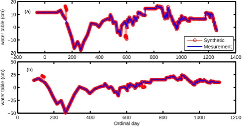
To test the responses of the different models to water table dynamics, we ran our models with the time series of water table depth artificially increased or decreased over a specific time period during the emission season. As shown in Fig. 4, for the Buck Hollow site, we increased the water table by 10 cm between ordinal day 150 and 160 (1 January 1991 was set to ordinal day 1), and decreased by 10 cm between ordi-nal day 590 and 600; for the Big Cassandra site, we increased the water table depth by 10 cm between ordinal day 135 and 145, and decreased by 10 cm between ordinal day 689 and

−200 0 200 400 600 800 1000 1200 1400

−20 −10 0 10 20

water table (cm)

(a)

0 200 400 600 800 1000 1200

−50 −25 0 25 50

Ordinal day

water table (cm)

(b)

Synthetic Mesurement

Fig. 4. The time series of water table depth used as driving data in this study at: (a) Buck Hollow site; (b) Big Cassandra site.

699. These days were chosen such that the differences of the CH4effluxes between the standard simulations and

sensitiv-ity simulations were significant enough to be identified. The results were analyzed by comparing simulations with those from standard simulations.

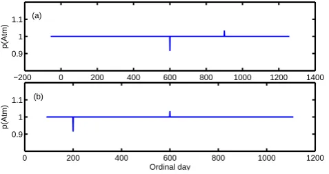
Two sets of experiments were used to test the model re-sponse to atmospheric pressure change. First, we conducted sensitivity simulations using a time series of artificially per-turbed low pressure or high pressure events (specifically 930 hPa low and 1045 hPa high) on two arbitrarily chosen days during the high-emission season in summer (Fig. 5). These two days were chosen based on the same criteria as that used in the water table sensitivity study. The effect of changing atmospheric pressure was analyzed by com-paring the change in pathways of CH4 transport with that

from the standard simulation. This was used to analyze whether the response is physically consistent or not. A sec-ond test was carried out to evaluate the overall effect of at-mospheric pressure variability using a time series of atmo-spheric pressure (Fig. 6) extracted from the European Centre for Medium-Range Weather Forecasts (ECMWF) Interim re-analysis dataset at the grid that encompassed the site for the same time period of measurement. The response was again analyzed by comparing the results to the standard simula-tions.

3 Results and discussion

3.1 Comparisons between standard model simulations and site-level observations

All models resulted in similar CH4fluxes (Table 2).

Specif-ically, for the Buck Hollow site, the S1, S2 and S4 mod-els all captured the temporal variability of the CH4 fluxes

Table 1. Parameters calibrated for standard model simulations.

ˆ

PCH4 PQ10 OˆCH4 Rveg

(mol m−3s−1) (None) (mol m−3s−1) (None)

Buck Hollow site

S1-model 3.5×10−7 12.7 1.10×10−7 1.2×10−3 S2-model 2.5×10−6 12.7 1.10×10−8 1.2×10−3 S4-model 1.25×10−6 12.7 1.10×10−8 1.2×10−3

Big Cassandra site

S1-model 7.5×10−8 6 1×10−7 1×10−3 S2-model 2.75×10−6 6 5×10−8 1×10−3 S4-model 1.375×10−6 6 1×10−7 1×10−3

−200 0 200 400 600 800 1000 1200 1400 0.9

1 1.1

Ordinal day

p(Atm)

(a)

0 200 400 600 800 1000 1200 0.9

1 1.1

Ordinal day

p(Atm)

(b)

Fig. 5. Synthetic atmospheric pressure used in simulations for sen-sitivity analysis at: (a) Buck Hollow site; (b) Big Cassandra site.

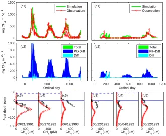
mean from an ensemble simulation of size four was shown for comparison. The S4 model performed best in terms of linear fitting and the root mean square error (RMSE) against the measurements (Table 2). The S1 model presented the second best results, with the simplest model structure. Over the three-year period, the simulated mean daily fluxes were 107.00 mg CH4m−2d−1, 168.82 mg CH4m−2d−1and

114.43 mg CH4m−2d−1, respectively by the S1, S2 and S4

model. The S2 model gave almost 50% higher emission than did the S1 and S4 model. In the S1 simulation, the max-imum production rate was at least an order of magnitude smaller than those of S2 and S4 models because it included no inhibition effect of O2on methanogenesis (Table 1). The

maximum oxidation rates (OˆCH4) were similar in magnitude.

Note that the simulations (except S4) were not very sensitive toOˆCH4.

The importance of different CH4transport pathways

var-ied in different models (Fig. 7a). Diffusion played a signif-icant role in the release of CH4 into the atmosphere, even

though plant transport remained the dominant pathway in S4 simulations. In S2 simulations, plant transport accounted for more than 90% of the efflux into the atmosphere. The

−200 0 200 400 600 800 1000 1200 1400

960 970 980 990 1000 1010 1020

Atmospheric pressure (hPa)

Ordinal day

Fig. 6. Transient atmospheric pressure used in simulations for sen-sitivity analysis. The same time series was applied at both sites, with truncation into proper time periods.

modeled diffusion contribution to efflux reached a short-term maximum between day 170 and 180 in the S1 simulations. This was due to a sudden and substantial decrease in wa-ter table from above the peat surface to below the peat sur-face (Fig. 4). This increased the concentration gradient of the CH4near the peat surface and thus increased diffusion.

Such short-term changes were also found in the S2 and S4 simulations, but with smaller magnitudes. All the models suggested that the efflux through ebullition was small, which agrees with measurements (Shannon and White, 1994). In the S4 simulation, the ebullition played a larger role than it did in S1 and S2 simulations.

S1 performed the best in simulating pore water concen-trations; followed by the S2 model and then the S4 model (Fig. 7a). For 12 June 1993, none of the models presented a satisfying result. The discrepancy might be due to the non-linearities of the transient simulations. For example, the pore water concentrations at a certain day were impacted by re-sults in previous days. Uncertainty in the driving data (e.g. soil temperature) is another source of such discrepancy.

0 500 1000 1500

mg CH

4

m

−2

d

−1

(a1) (b1)

0 500 1000 0

200 400 600 800 1000

Ordinal day

mg CH

4

m

−2

d

−1

(a2)

0 200 400 600 800 1000 1200 Ordinal day

(b2)

0 400 −150 −100 −50 0 50

09/21/1991

Peat depth (cm)

CH₄ (μM) (a3)

0 400 06/27/1992

CH₄ (μM) (a4)

0 400 06/12/1993

CH₄ (μM) (a5)

0 400 06/22/1991

CH₄ (μM) (b3)

0 400 06/04/1992

CH₄ (μM) (b4)

0 400 06/12/1993

CH₄ (μM) (b5) Simulation

Observation

Total Plt+Diff Diff

Simulation Observation

Total Plt+Diff Diff

Fig. 7a. Methane effluxes, component-wise emissions and pore water concentration profiles from one-substance model (S1 model) in the standard simulations. (a) Panels for the Buck Hollow site. (b) Panels for the Big Cassandra site. Dashed lines indicate the level of water tables.

0 500 1000 1500

mg CH

4

m

−2

d

−1

(c1) (d1)

0 500 1000 0

200 400 600 800 1000

Ordinal day

mg CH

4

m

−2

d

−1

(c2)

0 200 400 600 800 1000 1200 Ordinal day

(d2)

0 400 −150 −100 −50 0 50

09/21/1991

Peat depth (cm)

CH₄ (μM) (c3)

0 400 06/27/1992

CH₄ (μM) (c4)

0 400 06/12/1993

CH₄ (μM) (c5)

0 400 06/22/1991

CH₄ (μM) (d3)

0 400 06/04/1992

CH₄ (μM) (d4)

0 400 06/12/1993

CH₄ (μM) (d5) Simulation

Observation

Total Plt+Diff Diff

Simulation Observation

Total Plt+Diff Diff

0 500 1000 1500

mg CH

4

m

−2

d

−1

(e1) (f1)

0 500 1000 0

200 400 600 800 1000

Ordinal day

mg CH

4

m

−2

d

−1

(e2)

0 200 400 600 800 1000 1200 Ordinal day

(f2)

0 400 −150 −100 −50 0 50

09/21/1991

Peat depth (cm)

CH

4 (μM)

(e3)

0 400 06/27/1992

CH

4 (μM)

(e4)

0 400 06/12/1993

CH

4 (μM)

(e5)

0 400 06/22/1991

CH

4 (μM)

(f3)

0 400 06/04/1992

CH

4 (μM)

(f4)

0 400 06/12/1993

CH

4 (μM)

(f5) Simulation

Observation

Total Plt+Diff Diff

Simulation Observation

Total Plt+Diff Diff

Fig. 7c. Methane effluxes, component-wise emissions and pore water concentration profiles from four-substance model (S4 model) in the standard simulations. (e) Panels for the Buck Hollow site. (f) Panels for the Big Cassandra site. Dashed lines indicate the level of water tables.

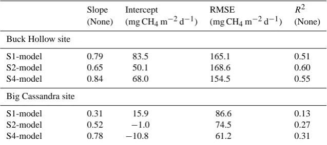
Table 2. Comparison of CH4efflux from the standard simulations to the measurements at the two Michigan peatlands. All statistics were

tested for significance and were found significant withp <0.001.

Slope Intercept RMSE R2

(None) (mg CH4m−2d−1) (mg CH4m−2d−1) (None)

Buck Hollow site

S1-model 0.79 83.5 165.1 0.51

S2-model 0.65 50.1 168.6 0.60

S4-model 0.84 68.0 154.5 0.55

Big Cassandra site

S1-model 0.31 15.9 86.6 0.13

S2-model 0.52 −1.0 74.5 0.27

S4-model 0.78 −10.8 61.2 0.31

model. Particularly for the second half year of 1991 and the year 1992, the results compared poorly with measurements. This underperformance may be due to an inadequate repre-sentation of the methanogenesis substrate, which was simu-lated in TEM but has not been specifically calibrated for wet-land ecosystems. For the three-year period, the mean daily fluxes were 42.51 mg CH4m−2d−1, 50.83 mg CH4m−2d−1

and 45.51 mg CH4m−2d−1, respectively, by the S1, S2 and

S4 models. Still, S2 simulated the highest CH4 emission

−100 0 100 200 300

mg CH

4

m

−2

d

−1

(a) S1

+

−

−100 −50 0 50 100

(b) S1

+

−

−100 0 100 200 300

mg CH

4

m

−2

d

−1

(c) S2

+

−

−100 −50 0 50 100

(d) S2

+

−

−100 200 500 800 1100 1400 −100

0 100 200 300

mg CH

4

m

−2

d

−1

(e) S4

Ordinal day

+

−

0 200 400 600 800 1000 1200 −100

−50 0 50 100

(f) S4

Ordinal day

+

−

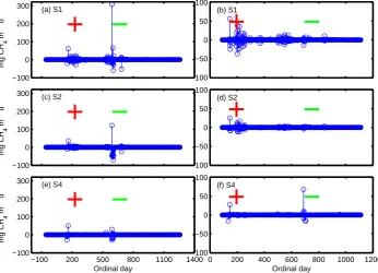
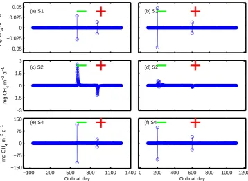
Fig. 8. Water table sensitivities with models of different complexities. Left-hand panels are for Buck Hollow site; right-hand panels are for Big Cassandra site. The red symbol “+” indicates the period of artificially increased water table depth, and the green symbol “−” indicates the period of artificially decreased water table depth.

3.2 Model sensitivity analyses

3.2.1 Sensitivity to water table change

We found that the response to a 10 cm change in surface standing water caused a change in the CH4efflux by as much

as−50∼300 mg CH4m−2d−1(Fig. 8). Such responses

de-pend on site characteristics and model complexity. At the Big Cassandra site, models S1 and S2 yielded a stronger re-sponse in effluxes to the water table increase than did the S4 model, while the opposite occurred for the water table decrease. At the Buck Hollow site, the responses of differ-ent models to the water table change were similar, but S1 gave a much stronger response to the water table decrease than did models S2 and S4. Nevertheless, all the models successfully predicted the retardation effect of an increase in surface standing water on CH4 efflux (Fig. 9). This can

be explained by the low diffusivity of gases in water relative to air. A higher column of surface standing water represents a longer distance of diffusion before gas can escape into the atmosphere. This phenomenon may account for CH4

accu-mulation in the peat column, which in turn enhances plant mediated transport and the oxidation of CH4 in the

rhizo-sphere, which decreases the efflux. When water table depth decreases, the diffusion distance is reduced, and efflux to the atmosphere increases (Fig. 9). In places where emergent vas-cular plants are sparse, a decrease in water table depth could enhance CH4efflux through ebullition. This was tested by

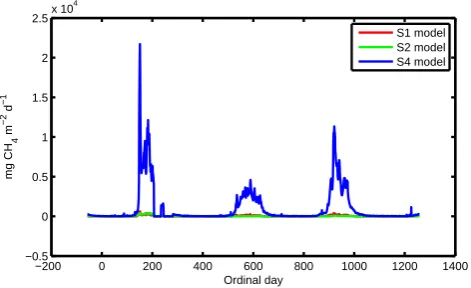
re-moving the plants and using the remaining parameters from Table 2 in the simulations. The results are shown in Fig. 10. We found that the S1 and S2 models had negligible ebulli-tion compared to that from model S4 in response to changes in water table. The burst of ebullition predicted by model S4 was more significant at the onset of a drop in standing wa-ter level. Then it decreased as the wawa-ter table continuously dropped and finally reached zero ebullition when the CH4

accumulation was too low to support ebullition. In contrast, the S1 and S2 models predicted that diffusion was the major pathway of CH4efflux and greatly underestimated the CH4

emissions through ebullition. Field data from Buck Hollow site also supported ebullition as important when the vegeta-tion is sparser (Shannon et al., 1996). These findings sug-gest that while models S1 and S2 performed relatively well with careful calibrations, the positive results were fortuitous. They represent an inadequate formulation but an artful pa-rameterization of the problem.

3.2.2 Sensitivity to atmospheric pressure change

−100 −50 0 50 100

mg CH

4

m

−2

d

−1 (a) S1

−100 0 100 200 300 _{(b) S1}

−100 −50 0 50 100

mg CH

4

m

−2

d

−1 (c) S2

−100 0 100 200 300 _{(d) S2}

140 150 160 170 180 −100

−50 0 50 100

mg CH

4

m

−2

d

−1 (e) S4

Ordinal day

580 590 600 610 620 −100

0 100 200 300 _{(f) S4}

Ordinal day

Fig. 9. Zoom-in plots for the water table sensitivity with models of different complexities at the Buck Hollow site. Left-hand panels were for the period where the water table depth is increased by 10 cm compared to the measured data, right-hand panels are for the period where the water table depth is decreased by 10 cm. The arrows indicate when the specified water table change starts and ends.

−200 0 200 400 600 800 1000 1200 1400 −0.5

0 0.5 1 1.5 2 2.5x 10

4

mg CH

4

m

−2

d

−1

Ordinal day

S1 model S2 model S4 model

Fig. 10. Methane effluxes through ebullition at the Buck Hollow site when no vegetation is present to support plant aided transport. See text for details.

atmospheric CH4 concentration is small, implying a small

change of the diffusion rate and thus the methane efflux in these two models. However, in the S4 model, the atmo-spheric pressure was further related to the ebullition fluxes. When a low atmospheric pressure occurred, the ebullition criterion became less restrictive, and bubbles were more eas-ily formed, enhancing the ebullition. In this simulation, a de-crease in atmospheric pressure could trigger an episodic in-crease in CH4efflux by as much as 120 mg CH4m−2d−1at

the Buck Hollow site and as much as 80 mg CH4m−2d−1at

the Big Cassandra site, comparable to the enhancement due to a decrease in surface standing water table depth.

Results from the sensitivity tests of transient atmospheric pressure were analyzed, which we found were very differ-ent with the differdiffer-ent models (see Fig. 12). For instance, in cases of low atmospheric pressure events at the Buck Hollow site, the S4 model usually predicted higher fluxes through en-hancement of ebullition. For the S1 model, response to atmo-spheric pressure change was negligible. The S2 model also responded significantly to the change of atmospheric pres-sure, but showed lower fluxes in accordance with a lower concentration of atmospheric CH4at the upper boundary. In

cases of high pressure events, S4 yielded reduced the fluxes by suppressing ebullition, S2 yielded enhanced fluxes due to a higher atmospheric concentration of CH4 at the upper

boundary, and S1 showed little response. Similar results were found at the Big Cassandra site. The change of atmo-spheric pressure also changed the rate of plant aided transport and diffusion. However, in our formulation of the algorithm, ebullition is the preferred route if it is triggered (which we also believe is true in the field, e.g. Tokida et al., 2005). By analyzing the cumulative differences, we found for the three-year period at the Buck Hollow site that the S4 model pre-dicted around 5% more emitted CH4using the transient

−0.05 −0.025 0 0.025 0.05

mg CH

4

m

−2

d

−1 (a) S1

−

+

−

+

−3 −1.5 0 1.5 3

mg CH

4

m

−2

d

−1 (c) S2

−

+

−

+

−100 200 500 800 1100 1400 −150

−75 0 75 150

mg CH

4

m

−2

d

−1

(e) S4

Ordinal day

−

+

0 200 400 600 800 1000 1200 (f) S4

Ordinal day

−

+

Fig. 11. Atmospheric pressure sensitivities with models of different complexities. (a), (c) and (e) panels are for Buck Hollow site; (b), (d) and (f) panels are for Big Cassandra site. The red symbol “+” indicates the day of artificially perturbed high pressure event, and the green symbol “−” indicates the day of artificially perturbed low pressure event. Note the scale of results from S4 model is 102of that from S2 model, and 103of that from S1 model.

less emission when the transient atmospheric pressure was used. Similar results were found for the Big Cassandra site, with smaller differences, in accordance with the lower emis-sion rates.

3.3 The importance of using temperature dependent parameters

In our standard and sensitivity simulations with the revised CH4 module, we treated the phase-related parameters, such

as diffusivities, Henry’s law constants and Bunsen coef-ficients as temperature dependent. Analysis showed that, within the typical temperature range (e.g.,−5 to 30◦C), the diffusivity of CO2in water changed±5%, the Henry’s law

constant and Bunsen coefficient changed±50% (results not shown). For CH4, its diffusivity in air changed±10% and

in water changed±5%, but the Henry’s law constant and Bunsen coefficient changed±40%. To test if fixing these parameters at a specific reference temperature could signif-icantly affect the results, we conducted a set of simulations with the phase-related parameter values corresponding to a reference temperature of 12.5◦C.

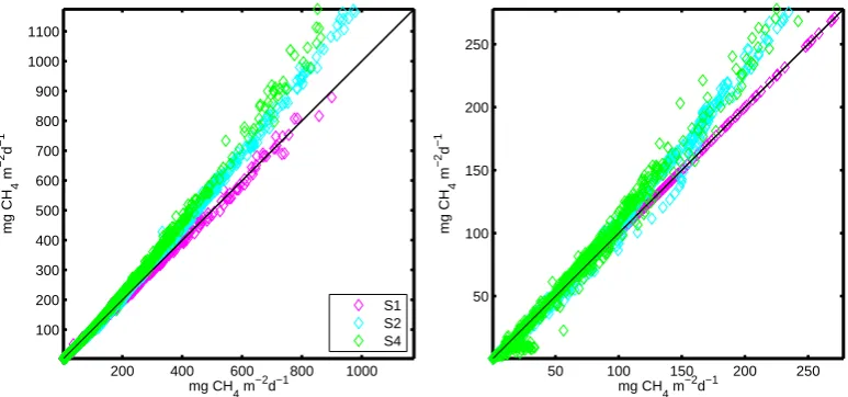
We found, for the S1 model, that the temperature depen-dence of these parameters did not change the efflux signif-icantly (Fig. 13). However, compared to the standard sim-ulation, both the S2 and S4 models predicted a higher CH4

efflux during high emission periods. Given that soil tures at the two sites were often above the reference tempera-ture during the high-emission summer season, the lower sol-ubility computed with the reference temperature allowed less O2and CH4to be stored in the soil, given almost the same

rate of CH4 production. Further, considering the inhibition

effect of O2on methanogenesis and the stimulus effect of O2

on methanotrophy, the higher emissions associated with the S2 and S4 models using coefficient values at the reference temperature is then explained as a stimulus of gas transport to the atmosphere. We conclude that fixing phase-related pa-rameters at their reference temperature values is safe for the S1 model, but that temperature-dependent parameters should be used in the S2 and S4 models.

3.4 The role of root density distribution

Previous CH4modeling has used a linear function for the

ver-tical distribution of root density (e.g., Walter and Heimann, 2000; Zhuang et al., 2004; also see Eq. (D2) in Appendix D). However, root biomass is often found to be exponentially distributed (Jackson et al., 1996), and an exponential root distribution could also be used (e.g., van Huissteden et al., 2006). Here we implemented both linear and exponential root distribution functions in our revised CH4module to test

−60 −30 0 30 60

Dif. (mg CH

4

m

−2

d

−1

)

(a) S1 model

S2 model S4 model

−8 −4 0 4 8

Cum. dif. (%)

(b)

−60 −30 0 30 60

Dif. (mg CH

4

m

−2

d

−1

)

(c)

−200 0 200 400 600 800 1000 1200 1400 −8

−4 0 4 8

Cum. dif. (%)

(d)

Ordinal day

Fig. 12. Differences in the response to transient atmospheric pressure and that to constant atmospheric pressure with models of different complexities. (a) Time series of the absolute difference at the Buck Hollow site. (b) Time series of cumulative difference at the Buck Hollow site. (c) Time series of the absolute difference at the Big Cassandra site. (d) Time series of cumulative difference at the Big Cassandra site. The difference is defined by subtracting the fluxes simulated with the standard 1 atm pressure from that using the transient atmospheric pressure data.

200 400 600 800 1000 100

200 300 400 500 600 700 800 900 1000 1100

mg CH

4

m

−2

d

−1

mg CH₄ m−2d−1

50 100 150 200 250 50

100 150 200 250

mg CH

4

m

−2

d

−1

mg CH₄ m−2d−1 S1

S2 S4

Fig. 13. Impact of temperature dependence of phase-related parameters on the CH₄efflux simulations with models of different complexities at: (a) Buck Hollow site; (b) Big Cassandra site. The black line denotes wherey=x. The results from standard simulations were plotted as

Table 3. Parameters calibrated for model simulations using a linear root distribution function.

ˆ

PCH4 PQ10

ˆ

OCH4 Rveg

(mol m−3s−1) (None) (mol m−3s−1) (None)

Buck Hollow site

S1-model 3.0×10−8 12.7 1.10×10−7 4.0×10−2 S2-model 2.0×10−6 12.7 1.10×10−8 4.0×10−2 S4-model 7.5×10−7 12.7 1.10×10−8 4.0×10−2

Big Cassandra site

S1-model 5.0×10−8 6 1×10−7 1.5×10−3 S2-model 1.5×10−6 6 5×10−8 1.5×10−3 S4-model 5.0×10−7 6 1×10−7 1.5×10−3

Table 4. Comparison of CH4efflux from the simulations using a linear root distribution function to the measurements at the two Michigan

peatlands. All statistics were tested for significance and were found significant withp<0.001, except those denoted in the parentheses.

Slope Intercept RMSE R2

(None) (mg CH4m−2d−1) (mg CH4m−2d−1) (None)

Buck Hollow site

S1-model 1.21 54.9 154.1 0.66

S2-model 0.78 47.9 139.8 0.64

S4-model 0.68 127.6 216.6 0.22

Big Cassandra site

S1-model 0.10 32.1 103.7 0.19 (p=0.2)

S2-model 0.10 26.5 183.6 0.07 (p<0.01)

S4-model 0.27 13.2 104.6 0.14

pore water concentrations. In both configurations, the pa-rameter values were obtained from calibration based on mea-surement data. The differences between the simulations were thus mainly due to the different model configurations.

We found the contributions from different pathways were different when two different root density distribution func-tions were used (Figs. 7a and 14a). In the standard simula-tion using an exponential root density distribusimula-tion funcsimula-tion, ebullition played a minor role, whereas in the simulation em-ploying a linear root density distribution, the ebullition was more significant, particularly in the S2 and S4 models. The ebullition was enhanced more at the Big Cassandra site than at the Buck Hollow site, suggesting that the responses of the models to two different root distribution functions are site dependent and related to the net CH4production

character-istics of the site. In the simulation employing the linear root distribution function, model-derived pore water CH4

concen-tration profiles underestimated field observations in the upper level of the peat column (Fig. 14a). The lower CH4

concen-trations ware due to a poor representation of transport in the

upper portion of the soil column when a linear root density function was used. Conversely, the exponential root distribu-tion extends smoothly down into depth of the peat column, producing more realistic pore water CH4concentration

pro-files. Therefore, though rigorous parameterization can lead to a good fit of the modeled CH4fluxes with respect to the

measurements, the model fails to capture other aspects of the measurements when an improper formulation of the problem is used. Also, in our case, the exponential distribution is a su-perior representation of root density as a function of depth. 3.5 Issues for regional application of the different

CH4models

The CH4models of different complexities developed in this

study can be used for regional hindcast and projection of wet-land CH4 emissions provided that necessary climate

forc-ing data are available. This is not a problem when these CH4models are used inside a biogeochemistry model, such

0 500 1000 1500

mg CH

4

m

−2

d

−1

(a1) (b1)

0 500 1000 0

200 400 600 800 1000

Ordinal day

mg CH

4

m

−2

d

−1

(a2)

0 200 400 600 800 1000 1200 Ordinal day

(b2)

0 400 −150 −100 −50 0 50

09/21/1991

Peat depth (cm)

CH₄ (μM) (a3)

0 400 06/27/1992

CH₄ (μM) (a4)

0 400 06/12/1993

CH₄ (μM) (a5)

0 400 06/22/1991

CH₄ (μM) (b3)

0 400 06/04/1992

CH₄ (μM) (b4)

0 400 06/12/1993

CH₄ (μM) (b5) Simulation

Observation

Total Plt+Diff Diff

Simulation Observation

Total Plt+Diff Diff

Fig. 14a. Methane effluxes, component-wise emissions and pore water concentration profiles from one-substance model (S1 model) in test simulations using a linear root distribution function. (a) Panels for the Buck Hollow site. (b) Panels for the Big Cassandra site. Dashed lines indicate the level of water tables.

0 500 1000 1500

mg CH

4

m

−2

d

−1

(c1) (d1)

0 500 1000 0

200 400 600 800 1000

Ordinal day

mg CH

4

m

−2

d

−1

(c2)

0 200 400 600 800 1000 1200 Ordinal day

(d2)

0 400 −150 −100 −50 0 50

09/21/1991

Peat depth (cm)

CH₄ (μM) (c3)

0 400 06/27/1992

CH₄ (μM) (c4)

0 400 06/12/1993

CH₄ (μM) (c5)

0 400 06/22/1991

CH₄ (μM) (d3)

0 400 06/04/1992

CH₄ (μM) (d4)

0 400 06/12/1993

CH₄ (μM) (d5) Simulation

Observation

Total Plt+Diff Diff

Simulation Observation

Total Plt+Diff Diff

0 500 1000 1500

mg CH

4

m

−2

d

−1

(e1) (f1)

0 500 1000 0

200 400 600 800 1000

Ordinal day

mg CH

4

m

−2

d

−1

(e2)

0 200 400 600 800 1000 1200 Ordinal day

(f2)

0 400 −150 −100 −50 0 50

09/21/1991

Peat depth (cm)

CH

4 (μM)

(e3)

0 400 06/27/1992

CH

4 (μM)

(e4)

0 400 06/12/1993

CH

4 (μM)

(e5)

0 400 06/22/1991

CH

4 (μM)

(f3)

0 400 06/04/1992

CH

4 (μM)

(f4)

0 400 06/12/1993

CH

4 (μM)

(f5) Simulation

Observation

Total Plt+Diff Diff

Simulation Observation

Total Plt+Diff Diff

Fig. 14c. Methane effluxes, component-wise emissions and pore water concentration profiles from four-substance model (S4 model) in test simulations using a linear root distribution function. (e) Panels for the Buck Hollow site. (f) Panels for the Big Cassandra site. Dashed lines indicate the level of water tables.

CH4 models can be computed explicitly when the

biogeo-chemistry model is driven by a climate dataset including air temperature, cloud fraction, precipitation and vapor pressure (Zhuang et al., 2004). The three CH4 models have almost

the same requirement for climate forcing, except that the S4 model requires surface pressure data for a better perfor-mance. For historical simulations, the surface pressure data can easily be obtained from various climate data sources, e.g. datasets from NCEP Reanalysis and ECMWF Interim Reanalysis. For projections, GCM model outputs would be a source for the necessary climate data. In some cases, when sea level pressure data rather than surface pressure data are output from GCMs (e.g. models involved in IPCC AR4, http://www.ipcc-data.org/ar4/gcm data.html). The sur-face pressure data can then be derived from a combination of sea level pressure data, information of air temperature, el-evation and vapor pressure (Wallace, 2006). Although the CH4models developed here have different complexities, they

have almost the same number of parameters that require cal-ibration. The more complicated S2 and S4 models have even fewer parameters to calibrate. For instance, the S2 and S4 models compute the fraction of CH4oxidation in the

rhizo-sphere explicitly – no parameterization is needed as in the S1 model.

The parameters of the CH4 models should be handled

carefully in regional applications. For instance, upscaling maximum CH4 production potential (PˆCH4) and maximum

CH4oxidation potential (QˆCH4) from the calibrated sites to

a region is critical. Currently, we use the maximum monthly NPP derived from a 50-year historical TEM simulation to scale the parameterPˆCH4and the maximum monthly soil

res-piration to scale the parameterQˆCH4. Both NPP and soil

res-piration are simulated with TEM. The extrapolation is based on the fact that CH4productivity is usually positively related

with NPP (e.g. Chanton et al., 1995), and CH4oxidation is

positively related with respiration (e.g. Nakano et al., 2004). The scaling is based upon the vegetation cover data. The re-maining model parameters derived from the calibrated site are used for our regional extrapolations. Thus, as a next step, we will test how different ways in extrapolating the site-specific parameters to a region affect the uncertainties in the wetland CH4 emissions quantified with the CH4 models of

different complexities. Also, an analysis of uncertainty due to equifinality will be attempted to investigate robustness of the parameterization from calibration at the limited number of sites (Tang and Zhuang, 2008).

The regional water table dynamics are another major source of uncertainty in quantifying regional wetland CH4

In particular, when the S4 model is used in regional simula-tions, there are grid cells, where vegetation is sparse, emitting CH4mainly via ebullition. In contrast, the S1 and S2

mod-els greatly underestimate the CH4 emissions in such cases

(e.g. Fig. 10). In these simulations, water table depths play a significant role in affecting CH4production, oxidation, soil

pressure profile, and diffusion process. To more accurately simulate water table dynamics, we are currently testing sev-eral different algorithms (e.g. Granberg et al., 1999; Weiss et al., 2006). The methane models with different complexi-ties will be further coupled with existing soil physics models (e.g. Zhuang et al., 2001, 2003; Tang and Zhuang, 2010) and with the tested water table depth model to conduct regional and global analyses of wetland CH4emissions.

4 Conclusions

We revised an extant process-based biogeochemistry model, the Terrestrial Ecosystem Model to account for the effects of multiple substances in a soil profile on CH4production,

oxi-dation, and transport. The new development allows CH4

ef-fluxes to be modeled with different levels of model complex-ity. When four-substances (O2, N2, CO2and CH4) are

con-sidered, the inhibitory effect of O2 on CH4 production and

the stimulatory effect of O2 on CH4oxidation are well

ac-counted for, and ebullition is modeled in a physically logical manner. When ebullition is modeled with a concentration-based threshold approach and the inhibition effect of O2

on CH4 production, and the competition for O2 between

methanotrophy and heterotrophic respiration are considered, the model becomes essentially a two-substance system. If we ignore the role of O2, while modeling bubble ebullition

with the concentration-based threshold function, the model is reduced to a one-substance system. These models were tested through a group of sensitivity analyses at two temper-ate peatland sites in Michigan. We showed that only the four-substance model with the new ebullition algorithm is able to account for the effects of a sudden drop in atmospheric pres-sure or in water table on episodic emissions. All models sim-ulated the retardation of CH4efflux after an increase in

sur-face standing water due to inhibited diffusion and enhanced rhizospheric oxidation. We conclud that, to more accurately account for the effects of atmospheric pressure dynamics and water table dynamics on methane effluxes, the four-substance model with the probabilistic but physics-based ebullition al-gorithm should be used in the future to quantify global wet-land CH4emissions. Further, to more accurately simulate the

pore water gas concentrations and different pathways of CH4

transport, an exponential root distribution function should be used and the phase-related parameters should be treated as temperature dependent.

Appendix A

The Henry’s law constants (unit: M atm−1_{) (Sander, 1999)}

are computed as

H=6.1×10−4exp

−1300

₁

T −

1 298.0

for N2 (A1)

H=1.3×10−3exp

−1500

₁

T −

1 298.0

for O2 (A2)

H=3.4×10−2exp

−2400

₁

T −

1 298.0

for CO2 (A3)

H=1.3×10−3exp

−1700

₁

T −

1 298.0

for CH4 (A4)

whereT is temperature (unit: K).

The Bunsen coefficient or solubility for gas i is related to Henry’s law constant as

αi=Hi× T

12.2 (A5)

The diffusivities (unit: m2s−1) (Frank et al., 1996; Arah and Stephen, 1998; Winkelmann, 2008) in air are computed as

Da=1.93×10−5×

_T

273.0

1.82

for N2 (A6)

Da=1.8×10−5×

_T

273.0

1.82

for O2 (A7)

Da=1.47×10−5×

_T

273.15

1.792

for CO2 (A8)

Da=1.9×10−5×

_T

298.0

1.82

for CH4 (A9)

The diffusivities (unit: m2s−1) in water are computed as

Dw=2.57×10−9×

_T

273.0

for N2 (A10)

Dw=2.4×10−9

_T

298.0

for O2 (A11)

Dw=1.81×10−6exp

_−2032.6 T

for CO2 (A12)

Dw=1.5×10−9×

_T

298.0

Appendix B

The maximum CH4production potential is defined as

P_CH∗ ₄= ˆPCH4f (SOM(z,t ))f (T (z,t ))f (pH(z,t ))f (Eh(z,t )) (B1)

wheref (SOM(z,t )),f (T (z,t )),f (pH(z,t )),f (Eh(z,t ))are

multiplier functions of methanogenesis substrate availability (modeled as a function of scaled NPP), soil temperature, pH value and redox potential, as defined in Zhuang et al. (2004).

ˆ

PCH4 (unit: mol m

−3_s−1_{) is a scaling parameter for model}

calibration. Another site specific parameter that needs cali-bration is theQ10coefficient (PQ10) off (T (z,t )).

The maximum CH4oxidation potential is defined as

O_CH∗

4= ˆOCH4f (T (z,t ))f (θ (z,t ))f (Eh(z,t )) (B2)

where f (T (z,t )), f (θ (z,t )), f (Eh(z,t )) are functions of soil temperature, soil moisture and redox potential (see Zhuang et al., 2004 for detailed descriptions). Parameter

ˆ

OCH4 (unit: mol m

−3_s−1_{) is calibrated for every}

represen-tative site. TheQ10 coefficient for temperature effect is set

to 2 throughout this study.

Appendix C

For the diffusive flux, the diffusion constant in Eq. (1) is de-fined for the bulk medium, which is conventionally computed (Stephen et al., 1998) as

Di =

1

τ

Di,a +αiθ Di,w

+αiθ

(C1) where subscripts a and w denote the diffusivity in air and in water (see Appendix A for ways of computation). τ is the tortuosity factor in the soil, taken as 1.5 throughout the study (Arah and Stephen, 1998).

For gas transport through the aerenchyma of wetland plants, we, following the argument in other studies (Teal and Kanwisher, 1966; Matthews et al., 2000; Segers and Leffe-laar, 2001), assumed the N2, CO2and CH4 are transported

in a similar way, such that

Ri=Ri∗(yi,a−yi,atm)=λrLvDi,af (t )(yi,a−yi,atm) (C2)

whereλr (unit: m air (m root)−1) is the specific

conduc-tivity of the root system andLv (unit: m root m−3soil) is

the root length density. A value of 3.0×10−4_{was used for}

λr. The vertical distribution of Lv in soil is assumed

fol-lowing the Gale-Grigal model (Jackson et al., 1996) (see the exponential model in Appendix D). The temporal variation

f (t )of the root is modeled similarly to Zhuang et al. (2004) and Walter and Heimann (2000). Also, we assumed the four gases can either be transported from the atmosphere to the roots or from the roots to the atmosphere. When the one-substance model is switched on, the oxidation of CH4in the

rhizosphere (Beckett et al., 2001) is not considered explicitly,

rather, as in Walter and Heimann (2000), we assume 50% of CH4is oxidized.

In the S4 model, the governing equation for CH4is

∂yCH4

∂t =

∂ ∂z

DCH4

∂yCH4

∂z

+ P

∗ CH4

1+ηyO2,w −Q∗_CH

4

yCH4,w

kCH4+yCH4,w

yO2,w

kO2+yO2,w −ECH4+R

∗

CH4 yCH4,atm−yCH4,a

(C3) for CO2is

∂yCO2

∂t = ∂ ∂z

DCO2

∂yCO2

∂z

+ P

∗

CH4

1+ηyO2,w

+Q∗CH4

yCH4,w

kCH4+yCH4,w

yO2,w

kO2+yO2,w

+V_R∗ yO2,w

kR+yO2,w

−ECO2+R

∗

CO2 yCO2,atm−yCO2,a

(C4) for O2is

∂yO2

∂t = ∂ ∂z

DO2

∂yO2

∂z

−2Q∗CH4

yCH4,w

kCH4+yCH4,w

yO2,w

kO2+yO2,w

−V_R∗ yO2,w

kR+yO2,w

−EO2+R

∗

O2 yO2,atm−yO2,a

(C5) and for N2is

∂yN2

∂t =

∂ ∂z

DN2

∂yN2

∂z

−EN2+R ∗

N2 yN2,atm−yN2,a

(C6)

Appendix D

The root length density in Eq. (C2) is defined as

Lv=Rvegf (z)= −Rveg×100log(β)β100z (D1)

whereβ is 0.943 for Buck Hollow Bog, and 0.910 for Big Cassandra Bog. Rvegis a scaling parameter needed in

cali-bration to account for differences in conducting capabilities for different plants. Note, the integrated root distribution function f (z) from lower boundary to soil surface equals one. The alternative root distribution used in Sect. 3.4, is defined as

f (z)=

2

Rd

1− z

Rd

for 0≤z≤Rd

0 otherwise (D2)

where Rd is root depth, computed using the Gale-Grigal

Symbol Definition Unit

αi Bunsen coefficient for substance i unitless

β coefficient for root distribution unitless

δ(s) Dirac delta function unitless

(z,t ) air-filled porosity m3air m−3soil

η inhibition coefficient of O2on methanogenesis m3water mol−1

θ (z,t ) soil moisutre m3water m−3soil

λr specific conductivity of the root system m air m−1root

τ tortuosity factor in the soil unitless

b pressure imposed by water column above water table (zwt<0)

or soil surface (zwt≥0) m

CH4,max threshold concentration for CH4ebullition mol m−3water

Di bulk diffusivity of substance i in soil m2s−1

Di,a diffusivity of substance i in air m2s−1

Di,w diffusivity of substance i in water m2s−1

E(z) total ebullition of the gases at depthz mol m−2

Ebi(z) potential ebullition of gas i at depthz mol m−2

H_i Henry’s law constant for substance i M atm−1

kCH4 Michaelis-Menten coefficient for CH4 mol m −3_water

kO2 Michaelis-Menten coefficient for O2 mol m −3_water

kR Michaelis-Menten coefficient for respiration mol m−3water

Lv root length density m root m−3soil

O2,max threshold concentration for O2ebullition mol m−3water

p atmospheric pressure Pa

P_CH∗

4 maximum CH4production potential mol m

−3_s−1

ˆ

PCH4 scaling parameter forP ∗

CH4 mol m

−3_s−1

POX fraction of CH4oxidized in rhizosphere unitless

PQ10 Q10coefficient for methanogenesis unitless

pr probability of bubble redissolution unitless

Ps(z,t ) total gas pressure at depthz, timet Pa

Ps,i(z,t ) partial gas pressure at depthz, timetby substance i Pa

P0 pressure scaling factor Pa

ˆ

p scaled atmospheric pressure unitless

Q∗_CH

4 maximum CH4oxidation potential mol m

−3_s−1

ˆ

QCH4 scaling parameter forQ ∗

CH4 mol m

−3_s−1

R_i∗ scaled rate of plant aided transport s−1

Rd root depth m

Rveg vegetation type dependent scaling parameter of gas conducting

capability unitless

V_R∗ maximum rate of respiration mol m−3s−1

yi bulk concentration of substance i mol m−3

yi,a gaseous concentration of substance i mol m−3air

yi,w aqueous concentration of substance i mol m−3water

yi,atm concentration of substance i in the atmosphere mol m−3air

˜

y_i equilibrium bulk concentration of substance i mol m−3

˜

yi,w equilibrium aqueous concentration of substance i mol m−3water

zwt depth of water table m

zs depth of soil surface m

z0 water depth scaling factor m