SRef-ID: 1432-0576/ag/2005-23-3055 © European Geosciences Union 2005
Annales
Geophysicae
Retrieving the solar EUV spectrum from a reduced
set of spectral lines
T. Dudok de Wit1, J. Lilensten2, J. Aboudarham3, P.-O. Amblard4, and M. Kretzschmar5
1LPCE, CNRS and University of Orl´eans, 3A avenue de la Recherche Scientifique, 45 071 Orl´eans cedex 2, France 2LPG, CNRS and Joseph Fourier University, Bˆatiment D de Physique, BP 53, 38 041 Saint-Martin d’H`eres cedex 9, France 3LESIA, Paris Observatory, 5 Place Jules Janssen, 92 195 Meudon, France
4LIS, CNRS, 961 Rue de la Houille Blanche, BP 46, 38 402 St. Martin d’H`eres cedex, France 5IFSI, INAF, Via del Fosso del Cavaliere, 00 133 Roma, Italy
Received: 22 February 2005 – Revised: 17 June 2005 – Accepted: 18 July 2005 – Published: 22 November 2005 Part of Special Issue “1st European Space Weather Week (ESWW)”
Abstract. The solar EUV irradiance is a key input for ther-mospheric and ionospheric models. Difficulties in continu-ously measuring the calibrated spectrum has prompted the use of various surrogate quantities. Although most proxies correlate quite well with the spectral variability, their use for modelling purposes becomes increasingly unsatisfactory. A different and data-driven approach is considered here, in which the EUV spectrum is reconstructed from a linear com-bination of a few, calibrated and carefully selected spectral lines. This approach is based on a statistical analysis of the temporal variability of EUV spectra, as recorded by the TIMED satellite. A basic set of lines is extracted, from which the salient features of the spectral variability can be recon-structed. The best results are achieved with a selection of 5 to 8 of these lines. This study focuses on the methodology for selecting these lines, which can also be used for instrument specification and provides new insight into the comparison of solar proxies against the EUV irradiance.
Keywords. Solar physics, astrophysics, and astronomy (ul-traviolet emissions) – Ionosphere (modelling and forecast; solar radiation and cosmic ray effects)
1 Introduction
1.1 General context
The solar ultraviolet (UV), extreme ultraviolet (EUV) and soft X-ray (XUV) irradiances1 are fundamental inputs for monitoring and forecasting the solar impact on the terrestrial environment. Any sudden variation in their intensity affects
Correspondence to: T. Dudok de Wit
(ddwit@cnrs-orleans.fr)
1It is common practice in aeronomy to range XUV from 1 nm to
30 nm (125 to 41 eV) and EUV from 30 nm to 121 nm (41 to 10 eV).
the ionosphere and thereby impacts on HF telecommunica-tions. The thermosphere is affected through heating and gas expansion, which have direct implications on orbitography. The forcing also acts indirectly on other layers of the atmo-sphere and may couple with the bioatmo-sphere (Wild et al., 2005). Most of these effects occur on a wide range of time scales, going from minutes (for eruptive phenomena) to days (the 27-day modulation caused by the solar rotation) and decades (the 22-year magnetic cycle) (Lean, 1991). They eventually influence longer-term global climate evolution (Fr¨ohlich and Lean, 2004).
The solar XUV and EUV spectral irradiances are also re-ceiving growing interest in the context of planetary upper at-mospheres. Recently, several studies have been devoted to the ionosphere of Mars (see Witasse et al., 2003) and of gi-ant planets.
To gain a better understanding of all these effects, spec-trally resolved solar XUV, EUV and UV irradiances must be monitored continuously, in real time and with sufficient radiometric accuracy for running thermospheric/ionospheric models. Such measurements suffer from a number of prob-lems. In particular, they must be carried out above the atmo-sphere and they are affected by instrumental limitations such as ageing. The resulting lack of data has generated a large “EUV hole” that has ended with the launch of the TIMED satellite (see below) in February 2002.
Following the inconclusive efforts to continuously mea-sure the EUV spectrum, various substitutes have been used as inputs for thermospheric/ionospheric models (Lathuill`ere et al., 2002). Best known are the F10.7 (radio flux at 10.7 cm) or the Mg II core-to-wing indices, both of which can be con-veniently measured from ground. Several experiments, how-ever, have revealed the lack of simple relationship between the F10.7 index and the EUV irradiance (Floyd et al., 2005). Not surprisingly, it has become increasingly difficult to meet the expectations of operational models with such proxies (see for example the studies by Witasse et al., 1999; Thuillier and Bruinsma, 2001). Yet, proxies continue to be used in space weather applications, both for convenience and by lack of handy and accurate UV data.
Most of the pre-2001 EUV models rely on a few experi-ments that were made onboard the Dynamics Explorer mis-sions (Hinteregger et al., 1973) and by rockets. Hintereg-ger (1981) and HinteregHintereg-ger et al. (1981) gave a first repre-sentation of Solar EUV irradiances for aeronomical appli-cations. A reference flux SC#21REF was assembled from measurements performed in July 1976, for weak solar activ-ity. An additional model (SERF 1) allowed the flux to be extended to other regimes of solar activity. Torr et al. (1979) and Torr and Torr (1985) proposed two reference fluxes for aeronomy called F79050N and SC#REFW. They divided the UV spectrum into 37 bins, some corresponding to intense spectral lines2. This work turned out to be extremely use-ful, partly because the authors provided the corresponding absorption and ionisation cross sections for major thermo-spheric species.
The main limitation of such models is the difficulty in es-timating the flux under various conditions of solar activity. In space weather applications, extreme conditions, which are the most difficult to model, are precisely the ones that are of interest. Several authors have tried since to take better advantage of the AE database. Two models are of special in-terest. Tobiska (1991) and Tobiska and Eparvier (1998) de-veloped a model called EUV, which takes inputs from other sources, such as the SME, OSO, and AEROS satellites, but also rockets and ground-based facilities. This model takes into account the solar emission zone of each spectral line, through a parameter. It also includes the F10.7 index as a proxy for the solar flux. A new version has recently been de-veloped (SOLAR2000), which uses the E10.7 index as proxy (Tobiska, 2001).
The other model of interest is EUVAC (Richards et al., 1994), which differs from EUV by the choice of the refer-ence flux and the interpolation formula. All these models are important for aeronomic computations. Although some have
2He II (25.63 nm), Fe XV (28.415 nm), Si XI (30.331 nm),
He II (30.378 nm), Mg IX (36.807 nm), Ne VII (46.522 nm), O VI (55.437 nm), He I (58.433 nm), O IV (59.960 nm), Mg X (60.976 nm), O V (62.973 nm), O III (70.336 nm), N IV (76.515 nm), Ne VIII (77.041 nm), O IV (78.936 nm), C III (97.702 nm), H I-Lymanβ(102.572 nm) and O VI (103.191 nm).
given good results, none of them can properly reproduce the variability at different wavelengths.
Warren et al. (1996, 1998) undertook a radically different approach. Their model, called NRLEUV, estimates the solar EUV irradiance from solar images in the Ca II K-line. The fraction of the solar surface that is covered by three types of regions (quiet Sun, coronal holes and active regions) is deter-mined. The corresponding spectra are estimated by first com-puting Differential Emission Measures (DEMs) from solar spectral line observations and then estimating from the DEM a typical EUV spectrum for each region, using a database such as CHIANTI. Optically thick lines and continua are di-rectly deduced from observations in each spectrum. Line intensities for coronal holes and active regions are deduced from from the Harvard instrument onboard Skylab, while the reference spectrum for the quiet Sun has recently been up-dated, using data from the SUMER and CDS instruments onboard SOHO (Warren, 2005). Once the area covered by each of the three regions is known, the EUV irradiance spec-trum and its variability can be reconstructed.
1.2 Purpose of this study
Recently, Kretzschmar et al. (2005) investigated the possi-bility of reconstructing the solar EUV irradiance spectrum from a linear combination of a small set of (typically 6) mea-sured spectral lines. Their selection was based on a detailed comparison between synthetic spectra and the computed dif-ferential emission measure. Assuming that a calibrated spec-trograph continuously measures the irradiance of a few, care-fully selected emission lines, the authors determined the best candidates for this. Such an instrument would be much easier to operate than a spectrometer that covers the full spectrum.
The present work is a continuation of that study, with a dif-ferent approach. Instead of using physics-based models, we follow a data-driven approach that is based on two years of EUV spectra as measured by the Solar Extreme Ultraviolet Experiment (SEE) (Woods et al., 2005) onboard the Ther-mosphere Ionosphere Mesosphere Energetics and Dynamics (TIMED) satellite.
This study is organised as follows: the data set and its pre-processing are presented in Sect. 2. Exploratory statistical analyses of these data are discussed in Sect. 3. Additional considerations are used in Sect. 4 to help select a set of 14 spectral lines. Various reconstructions of the spectrum are presented in Sect. 5 for a typical case where 6 lines are used. All other combinations of 1 up to 10 lines are discussed in Sect. 6.
2 Choice of the data set
This study is based on more than two years of daily-averaged solar spectral irradiance data from the EUV Grating Spectro-graph (EGS), which is part of the Solar Extreme Ultravio-let Experiment (SEE) (Woods et al., 2005) onboard TIMED. The EGS spectrograph covers the spectral range from 26 to 194 nm at 0.4 nm spectral resolution; our analysis is based on daily averaged spectra that are publicly available from the web and are interpolated to 0.1 nm intervals3. SEE observes the Sun for about 3 min per orbit of 97 min, so the contri-bution from flares can be subtracted. Additional corrections are made for atmospheric absorption and instrument degra-dation, and the spectra are normalised to 1 AU.
Our training set includes all spectrograph channels except some that are corrupted by instrumental artefacts or by higher order emission from bright lines. There are no channels in the 114–120 nm and 123–129 nm ranges because a filter blocks out the bright H I Lyman-αemission. This brings the total number of channels to 1551.
This data set continuously covers the period ranging from the start of the scientific exploitation on 8 February 2002 un-til 28 July 2004. Some channels show degradations starting early 2004. We use the full data set (902 days) when this degradation has no incidence on the analysis, and a shorter time span (657 days) otherwise. Both spans cover a substan-tial fraction of the declining solar cycle.
It is essential for our study that the data set covers a long period in order to properly capture the dynamics of the EUV spectrum. Ideally, one solar cycle would be needed. No such homogeneous data set exists, so we carried out several tests to check that our conclusions are not significantly af-fected by the lack of coverage. In particular, we checked for differences between results obtained from the first half only (i.e. solar maximum) and the second half (declining phase) of the data set, but did not find any significant ones. In spite of this, the lack of temporal coverage remains a major limitation against investigating long-term effects such as asymmetries between rising and declining phases of the solar cycle. Our conclusions may therefore change a little once longer time series become available.
In the same way, our results reflect the spectral range and the resolution that are imposed by the EGS instrument. Re-stricting the analysis to a subset of that range will not sig-nificantly affect the results of our classification study. An 3These level 3 data (version 7) are available from http://lasp.
colorado.edu/see/
2002 2003 2004
−0.5 0 0.5
amplitude vs mean value
year
Fe XVI
Mg X
C III
H I
Si II
Wolf sunspot nr
F10.7 index 33.54 nm
60.98 nm
97.70 nm
121.57 nm
[image:3.595.310.547.61.246.2]181.69 nm
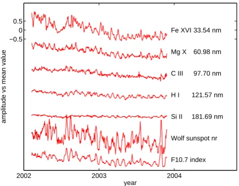
Fig. 1. Time evolution of five spectral lines (as measured by
TIMED) and two proxies for solar activity. All time series are nor-malised to their time average. Note that the 27-day modulation, caused by solar rotation, has a much larger amplitude in the coronal Fe XVI line than in the chromospheric Si II line.
extension toward longer wavelengths or toward smaller ones (using for example the XUV photometers of SEE), however, is likely to add novel features. We did not attempt yet to in-corporate such data from other instruments, as the analysis of an inhomogeneous data set requires considerably more care. Clearly, our approach cannot be used to reconstruct spectra with a better resolution than what SEE can offer. If, however, one would like to reconstruct spectra using an instrument that has a broader passband (such as a radiometer), then we just have to convolute the SEE data with the detector response. If the specifications of the latter are sufficiently well known, then the reconstruction problem remains unchanged and our method still applies.
A time-averaged EUV spectrum is shown in Fig. 2. For the purpose of our study, we start with a preselection of the 38 most intense and well-identified spectral lines. Since our final objective is the reconstruction of the spectral irradiance, we shall not make any distinction between the contribution of the lines and that of the continuum, even though the underly-ing physics differs substantially. We did repeat our analysis after subtracting the continuum; although this gave interest-ing insight into the physics of the continuum, it did not affect our line selection. Those results will be discussed in a forth-coming publication.
3 Exploratory statistical analysis of the EUV spectrum
20 40 60 80 100 120 140 160 180 200 10−6
10−5 10−4 10−3 10−2 10−1
λ [nm]
average flux [W/m
2 /sec/nm]
Fe XV
He II
Fe XVI
Fe XVI Mg IX
Fe XV Ne VII
Si XII
Si XII
He I
O IV
He I
Mg X
O V
O III N IV Ne VIII
Ne VIII
O IV
O II
H I H I C III H I
O VI
O VI
N II
H I
O I
C II
Si IV
Si IV
C IV
C I He II
C I
[image:4.595.115.479.64.249.2]Si II Si II
Fig. 2. Time-averaged EUV spectrum from the EGS instrument. The 38 strong spectral lines are highlighted.
100 101 102
88 90 92 94 96 98 100
number of variables i
[image:4.595.50.285.285.437.2]cumulative energy [%]
Fig. 3. Cumulative energy (in %) of the 100 dominant pairs of
vari-ables, out of 657. The horizontal axis is logarithmic, revealing an inflexion aroundk=4−6, which can be interpreted as the number of significant variables.
3.1 Determining the number of spectral lines
The first quantity of interest is the number of spectral lines that is needed to satisfactorily reconstruct the full spectrum by linear combination. This is a optimisation problem, for which insight can be gained from Principal Component Anal-ysis (Mardia et al., 1980; Chatfield and Collins, 1990), also known as Singular Value Decomposition (SVD) (Golub and Van Loan, 2000). The SVD is commonly used in multivari-ate statistics to replace an ensemble of correlmultivari-ated variables by a smaller set of new variables, called principal components, whose linear combination captures the main features of the original data.
Let I (λ, t ) denote the solar flux intensity measured at timet and wavelengthλ. Using the SVD, this flux can be transformed into a unique set of uncorrelated variablesfi(λ)
andgi(t )that are derived in decreasing order of importance
(see Appendix A).
I (λ, t )= N
X
i=1
Wi fi(λ) gi(t ) .
The variables fi(λ) andgi(t ) are normalised so that each
weight squaredWi2measures the amount of energy (or vari-ance) of the data that is explained by the corresponding pair of variables. Heavily weighted pairs describe coherent pat-terns and thus capture salient features of the data. Weakly weighted pairs in contrast describe local variations in time and in wavelength. The number of large weights therefore is indicative of the effective number of degrees of freedom that is at play, and has frequently been interpreted as such, see for example Ciliberto and Nicolaenko (1991). The physical interpretation of this quantity, however, should not be over-looked, as the linear decomposition of the spectral variability into uncorrelated modes has no sound physical justification.
The interpretation of the energies can be simplified by nor-malising them
Ei = Wi2
PN j=1Wj2
and subsequently computing their cumulative sum. This quantity indicates how many variables are needed to describe a given fraction of the total variance; it is displayed in Fig. 3. We applied the SVD to the full spectral matrix, after nor-malising each channel to its time average. The reason for this choice will be explained later. The distribution of the weights indicates that less than ten variables (out of 657) are actually needed to describe the salient properties of the full spectrum. Figure 3 shows that one pair of variables already captures more than 88% of the energy of the normalised flux, two pairs capture almost 92%, three pairs 94%, etc. This result vividly illustrates the strong redundancy of the spectral vari-ability. The SVD gives us quantitative evidence and thereby justifies the selection procedure that follows.
be needed, depending on the required accuracy. An analysis based on information theoretic criteria (Dudok de Wit, 1995) suggests that 6 variables is a reasonable choice.
By performing the SVD, we assume that the spectrum can be decomposed into linear combinations of many channels. This is not exactly what we want, since we are looking for a linear combination of selected channels only. The cumulative energy displayed in Fig. 3 therefore remains merely indica-tive and a different criterion will be introduced in Sect. 5. 3.2 Measuring the dissimilarity between lines
Our next objective is to identify those spectral lines from which the full spectrum can most easily be reconstructed. To do so, we first look for families or clusters of similar lines and then discard all redundant lines. Two lines are consid-ered to be similar or redundant if the temporal evolution of their flux, when suitably normalised, is the same. Next, we represent each line by a single point on a 2-D map, in such a way that the distance between pairs of lines reflects their dissimilarity. Such a map clearly reveals clusters and also provides additional insight into the physics. The appropriate method for this is called multidimensional scaling (Mardia et al., 1980; Chatfield and Collins, 1990).
A familiar example of multidimensional scaling can be found in atlases, which often contain tables that list the short-est distance between pairs of cities. Using multidimensional scaling, one can reconstruct the shape of a country directly from such tables. The results are of course relative, insofar the resulting map can be rotated, translated or reflected.
A crucial step in multidimensional scaling is the choice of the measure of dissimilarity. Two natural choices here are the Euclidean distanced between time-averaged fluxes, and between standardised fluxes
d(i, j )=
s X
t
φ (λi, t )−φ (λj, t )
2 ,
where
φ (λ, t )=I (λ, t )− hI (λ, t )it
hI (λ, t )it the time-averaged flux
or
φ (λ, t )=I (λ, t )− hI (λ, t )it σIλ
the standardised flux.
h· · ·it denotes time averaging4, andσIλ is the standard devi-ation of the flux. A normalisdevi-ation is compulsory since we are interested in comparing temporal dynamics, not absolute intensities.
Standardisation is the default normalisation in statistical analysis. Although this choice has the advantage of putting all irradiances on equal footing, it also destroys all informa-tion about the level of variability, which is an important input for thermospheric/ionospheric models. As shown by Fig. 1, 4Other measures such as the median can be used, but they do not
improve the results significantly.
coronal lines usually exhibit a much stronger variability than chromospheric lines. There are two reasons why we prefer here a normalisation versus time-average. First, it retains the level of variability. Second, it requires knowledge only of the time-averaged irradiance and is therefore less prone to reconstruction errors.
Multidimensional scaling is a computationally straightfor-ward technique, which merely involves a few matrix opera-tions. Incidentally, since we are using Euclidean distances, the locations on the 2-D map can be computed in a sin-gle step, using the SVD (Chatfield and Collins, 1990). Let φ (λ, t )=PN
i=1Wifi(λ)gi(t )be the SVD of the normalised
fluxes, thenWifi(λ)directly gives us the coordinates of the
different wavelengths along thei0th axis. The total number of modes isN=657, so the dimension of the phase space is also 657. Most dimensions, however, are irrelevant since only the very first axes carry significant weights. The first axis carries 78.5% of the variance, the two first axes 91.7%, the three first axes 94.0%, the four first axes 95.1%, etc. We conclude that two dimensions already capture the salient features; a third axis does not add much information and merely com-plicates the visualisation. This remarkable result is a direct consequence of the redundancy of the spectral dynamics.
The distance map of the normalised fluxes is displayed in Fig. 4, with colours reflecting the channel wavelength. The most important result is that each channel can be approxi-mated by a single point on a 2-D map, in such a way that the distance between two points reflects the dissimilarity in their time evolution. This reduction of the full spectral dynamics to a 2-D map considerably eases our analysis. It also allows us to compare all the lines in a single glance, in contrast to usual tables of correlation coefficients.
Figure 4 reveals a clear structure, with some natural group-ings. The most conspicuous cluster of points occurs near the far right, where all the least energetic channels tend to be-have similarly. The most energetic channels are located in the opposite corner; their more erratic distribution suggests that each line has a specific dynamics. This plot also sug-gests that the intense spectral lines (marked with a circle) and the remainder of the spectrum, including the continuum, do not behave very differently. Outliers either correspond to hot coronal lines, to mixtures of unresolved lines, or to some channels that have a low signal-to-noise ratio.
Let us stress that neither the axes of this map nor the units of measurement are important for our purposes; what mat-ters is the relative distance between points. A finer analysis, however, reveals that the horizontal axis captures differences in the way channels evolve on the long term, with a time scale of the order of years. The vertical axis on the contrary describes differences in the way they are modulated by the 27-day solar period and its first harmonic. This suggests that the distance map has naturally succeeded in separating two dominant scales that occur in the variability.
40 60 80 100 120 140 160 180
−10 −8 −6 −4 −2 0
−5 −4 −3 −2 −1 0 1 2 3 4
axis 1
[image:6.595.51.286.63.316.2]axis 2
Fig. 4. 2-D map of the normalised fluxes. The distance between two
points is indicative of the dissimilarity between the corresponding fluxes. The colour code corresponds to the wavelength in nm ; the 38 strong spectral lines that are labelled in Fig. 2 are circled. Axis 1 corresponds toW1f1(λ)and axis 2 toW2f2(λ).
2-D map in Fig. 5, now using a colour code that reflects the characteristic emission temperature (i.e. the temperature at which the ionisation equilibrium curve peaks, Arnaud and Raymond, 1992).
Figure 5 reveals a weak ordering of the spectral lines, with the hot coronal ones on the left, and most chromospheric and transition region lines on the right. Temperature a priori does not seem to be a governing parameter. Some lines that is-sue from different altitudes, such as the chromospheric He I line at 58.43 nm and the coronal Mg X line at 60.98 nm, for example, are remarkably close. One can indeed verify that their temporal dynamics are very similar. Many effects can explain this departure from a simple temperature ordering. Some are instrumental, while others are physical:
– Instrumental artefacts: instrumental effects such as higher order emission are likely to affect the location of some lines such as Mg X at 60.98 nm, which is pol-luted by second order emission of the strong He II line at 30.38 nm. Such effects tend to bring lines closer to-gether.
– Blending: the EGS instrument cannot resolve nearby spectral lines such as He II at 30.38 nm and the Si XI line at 30.33 nm. This blending may partly explain the peculiar location of the chromospheric He II line amidst hotter coronal lines.
– Physics of the emission processes: the emission tem-perature clearly does not suffice to describe the condi-tions under which a line is emitted. Some lines are elec-tron number density or temperature dependent, while others are not (Mariska, 1993). For some chromo-spheric lines such as He I at 58.4 nm, the emission is ac-tually driven by coronal photons. This effect contributes to displacing such lines to the left of the 2-D map. – Optical depth: once optically thick lines (such as He
I, He II and H I), are removed from Fig. 5, an al-most monotonic variation of the temperature is observed along the horizontal axis. Optical thickness therefore strongly affects the variability. The EGS instrument cannot resolve the core and the wings of thick lines, whose location on the 2-D map averages over a variety of complex emission mechanisms.
Our 2-D projection of course masks finer details that show up in higher dimensions. Adding a third dimension intro-duces a (very weak) scatter, whose physical interpretation is still unclear to us. The even weaker fourth dimension cap-tures an unsuspected periodic spectral shift whose origin was identified as the consequence of small instrument tempera-ture changes caused by orbit precession.
Figure 5 also suggests that the continuum has little im-pact on the dynamics of spectral lines. The two Si XII lines at 49.94 and 52.07 nm for example, coincide, even though the contribution of the He continuum to the second is much larger. The consequences of all these results for solar physics will be elaborated upon in a forthcoming paper.
Another interesting exercise consists in comparing the fluxes against various indices of solar activity. Solar indices are routinely used as surrogates for EUV irradiances (Floyd et al., 2005). Four such proxies are shown in Fig. 5, using the same normalisation as for the irradiances. They are the:
– International sunspot index or number (from the SIDC, Royal Observatory of Belgium, Brussels);
– F10.7 decimetric index: the daily Penticton solar radio flux at 10.7 cm (from the SEC, NOAA, Boulder); – E10.7 index: derived from the F10.7 index (Tobiska,
2001), and used for ionospheric models (from Space Environment Technologies);
– Mg II index: core-to-wing ratio of two singly ionised magnesium lines, at wavelengths of 280.2 nm (Mg II h line) and 279.5 nm (Mg II k line). This proxy was first developed from Nimbus-7 SBUV spectral scan ir-radiance data by Heath and Schlesinger (1986). The data are from the Global Ozone Monitoring Experiment (GOME), version 2.1 (Weber et al., 1995).
4 4.5 5 5.5 6
−10 −8 −6 −4 −2 0
−2 0 2 4 6
f s
e
m
axis 1
axis 2
Fe XVI
33.5
Fe XVI
36.1
Fe XV
41.7
Fe XV
28.4
Si XII
49.9
Si XII
52.1
Mg X
61
He I
58.4
He II
30.4
Mg IX
36.8
O VI
103.2
H I
102.6
C III
97.7
O VI
103.8
He I
53.7
N II
108.5
H I
95
H I
93.8
Ne VIII
77
Ne VIII
78
O V
63
H I
121.6
Ne VII
46.5
O IV
55.4
C II
133.5
O III
70.4
O II
83.4
Si IV
139.4
N IV
76.5
Si IV
140.3
O IV
78.8
C IV
154.9
He II
164
C I
165.7
C I
156.1
O I
130.4
Si II
181.7
Si II
[image:7.595.119.484.65.460.2]180.8
Fig. 5. Same 2-D representation as in Fig. 4, but only 38 strong lines are highlighted. The colour code refers to the decimal logarithm of
the emission temperature [K]. Letters refer to various proxies: s (international sunspot number), f (F10.7 radio flux), m (MgII core-to-wing index) and e (E10.7 index). The 14 reference lines to be used later in this study are circled.
are located closer to more energetic lines, but definitely re-main outside of the cloud of points. This confirms the dif-ficulties encountered in reconstructing the EUV irradiance using F10.7 (Thuillier and Bruinsma, 2001). The same holds for the sunspot number, which is the worst by our standards. The location of these non-radiometric proxies with respect to the spectral lines is a clear illustration of their differing phys-ical origin. We conclude that none of the proxies correctly describes that part of the EUV spectrum which is important for thermospheric modelling.
Another property of the 2-D is worth mentioning. Because of the Euclidean geometry, any linear combination of two proxies or lines will be located on a straight line linking their locations on the map. A linear combination of the Mg II and F10.7 indices, for example, will reasonably well fit the H I Lyman-αline, but certainly not a hot coronal line. The 2-D map is in this sense a powerful visual tool for assessing the validity range of proxies. Incidentally, we can already
con-clude from that three is the minimum number of references needed to reasonably fit the full spectrum. As we shall see later, this figure is not far from the true answer.
Let us conclude with two remarks. First, the location of the points in Fig. 5 may change a little as data from solar mini-mum become available. Second, this representation can also be used to compare composite quantities, such as the output of instruments with given passbands, such as radiometers.
3.3 Selecting the lines by classification analysis
0 1 2 3 4 5 6
C I 165.7
Si II 181.7
C I 156.1
Si II 180.8
O I 130.4
C II 133.5
Si IV 139.4
Si IV 140.3
C IV 154.9
He II 164
O III 70.4
N IV 76.5
O IV 78.8
O II 83.4
Ne VII 46.5 Ne VIII 77 Ne VIII 78
He I 53.7
H I 93.8
H I 95
N II 108.5
O VI 103.8
O IV 55.4
O V 63
H I 121.6
C III 97.7
H I 102.6
O VI 103.2
He II 30.4
Mg IX 36.8 Mg X 61
He I 58.4
Fe XV 28.4 Fe XV 41.7 Si XII 49.9 Si XII 52.1 Fe XVI 33.5 Fe XVI 36.1
[image:8.595.52.286.63.328.2]distance
Fig. 6. Dendrogram of the 38 spectral lines using an average
dis-tance linkage between all lines. The colour code associated with each line is indicative of the characteristic temperature, using the same scaling as in Fig. 5.
Some guidance may be obtained here from the dendro-gram or hierarchical structure tree (Chatfield and Collins, 1990). A dendrogram is a diagrammatical representation of the hierarchical structure of the spectral lines, in which one axis represents the distance between each pair of lines. Fig-ure 6 shows the dendrogram computed from the average dis-tance between each pair of spectral lines.
According to Fig. 6, the dissimilarity between the Fe XV line at 28.4 nm and the Si XII line at 52.1 nm is about 2 units, as given by the length of the horizontal segment one has to travel in order to go from one line to the other. The ordering of the spectral lines on the far right of the dendrogram is of little importance. The main features of interest are clusters of spectral lines that are linked by long horizontal segments. One can readily distinguish two such clusters, one of which contains the 6 hottest lines. Many smaller clusters are appar-ent, but their significance is often questionable.
To partition the lines into, say, 6 clusters, we draw a verti-cal line and move it to the right until exactly 6 branches are intersected. One representative spectral line must be chosen among each of the following 6 clusters:
1 2 3 4 5 6
0 50 100 150 200
10−6 10−5 10−4 10−3 10−2 10−1
λ [nm]
average flux [W/m
2/sec/nm] axis 1
[image:8.595.310.545.63.250.2]axis 2
Fig. 7. Clustering analysis of the EUV spectrum: each channel is
labelled with a colour corresponding to one of the 6 clusters it lies closest to. The six clusters are those given by the dendrogram. The insert shows where the clusters are located on the 2-D map.
cluster 1 Fe XVI (33.5 or 36.1 nm) cluster 2 Si XII (49.9 or 52.1 nm)
or Fe XV (28.4 or 41.7 nm) cluster 3 He I (58.4 nm)
cluster 4 Mg X (61.0 nm), Mg IX (36.8 nm) or He II (30.4 nm)
cluster 5 O VI (103.2 nm) to Ne VII (46.5 nm) cluster 6 O II (83.4 nm) to C I (165.7 nm)
The distinction between clusters 3 and 4 is barely signif-icant, as a small change in the data set may lead to a re-ordering of the lines or to their merging into a single cluster. Dendrograms therefore leave considerable freedom as to the choice of the best partition.
To illustrate this partitioning, we show in Fig. 7 the results of a partitioning of into 6 clusters. A number is assigned to each channel, given by its closest cluster centre. Such a rep-resentation is often useful for an exploratory analysis. Clus-ter 5, for example, mostly captures channels that are dom-inated by H I emission, whereas cluster 6 is domdom-inated by weakly energetic emission. Cluster 4 is more representative of the He continuum.
3.4 More selection criteria
Table 1. The 14 lines that are adequate for reconstructing the solar
EUV spectrum from 26 to 194 nm.
He II (30.38 nm) He I (58.43 nm) O I (130.43 nm) Fe XVI (33.54 nm) O III (70.38 nm) C II (133.51 nm) Fe XV (41.73 nm) O II (83.42 nm) C IV (154.95 nm) Ne VII (46.52 nm) C III (97.70 nm) Si II (181.69 nm) O IV (55.43 nm) H I (121.57 nm)
– have the lowest intensity (to enhance the signal-to-noise ratio);
– are blended by nearby strong lines (to avoid complex behaviour);
– have a broad peak (to avoid difficulties in determining the quantities such as the position of the maximum, the FWHM, etc.);
– may suffer from instrumental artefacts, such as pollu-tion by higher order emission from a strong line. The Mg X line at 60.98 nm is one of them.
With these constraints, our set reduces to 14 lines, see Ta-ble 1. We kept the Ta-blended He II line at 30.38 nm because it is one of the most common and enduring lines. Our new set includes all the lines that are needed to cover the cloud of points in Fig. 5. It provides a homogeneous coverage of the different emission temperatures at the Sun, as shown in Fig. 8; it also incorporates all the lines that are traditionally used in thermospheric modelling, such as He II (30.38 nm), O II (83.42 nm) and C III (97.70 nm). This set, however, is still redundant, so the selection must continue until fewer lines remain.
3.5 Conclusions of the exploratory analysis
The picture that emerges from this exploratory analysis is a strong redundancy of the spectral variability, owing to which most of the dynamics can be described by the location of the lines on a 2-D map that covers the two dominant degrees of freedom. From this we conclude that the full spectrum can be reproduced with a small set of (much less than 10) spec-tral lines. Most lines belong to larger clusters, in which all but one representative line can be discarded. Some lines on the contrary stand out by their unique dynamics, such as Mg X (61.0 nm) and Fe XVI (36.1 nm). Emission temperature is an important parameter here, but many other physical and instrumental effects contribute to the location of the points. These “outsiders” deserve special attention and ought to be included in the reconstruction procedure if one aims at mod-elling all wavelengths equally well5.
5When trying to reconstruct the EUV spectrum, we assume that
these lines are optically thin. Of course, this is not true for lines of the first Lyman series, some Carbon lines, etc.
40 60 80 100 120 140 160 180 103
104 105 106 107
λ [nm]
temperature [K]
Fe XV
He II
Fe XVI Fe XVI
Mg IX
Fe XV
Ne VII
Si XII Si XII
He I O IV He I Mg X O V O III N IV
Ne VIII Ne VIII
O IV
O II
H I H I
C III
H I
O VI O VI
N II
H I O I
C II
Si IV Si IV
C IV
C I
He II
C I
Si II Si II
Fe XV
He II
Fe XVI Fe XVI
Mg IX
Fe XV
Ne VII
Si XII Si XII
He I O IV He I Mg X O V O III N IV
Ne VIII Ne VIII
O IV
O II
H I H I
C III
H I
O VI O VI
N II
H I O I
C II
Si IV Si IV
C IV
C I
He II
C I
Si II Si II
Fe XV
He II
Fe XVI Fe XVI
Mg IX
Fe XV
Ne VII
Si XII Si XII
He I O IV He I Mg X O V O III N IV
Ne VIII Ne VIII
O IV
O II
H I H I
C III
H I
O VI O VI
N II
H I O I
C II
Si IV Si IV
C IV
C I
He II
C I
Si II Si II
Fe XV
He II
Fe XVI Fe XVI
Mg IX
Fe XV
Ne VII
Si XII Si XII
He I O IV He I Mg X O V O III N IV
Ne VIII Ne VIII
O IV
O II
H I H I
C III
H I
O VI O VI
N II
H I O I
C II
Si IV Si IV
C IV
C I
He II
C I
Si II Si II
Fe XV
He II
Fe XVI Fe XVI
Mg IX
Fe XV
Ne VII
Si XII Si XII
He I O IV He I Mg X O V O III N IV
Ne VIII Ne VIII
O IV
O II
H I H I
C III
H I
O VI O VI
N II
H I O I
C II
Si IV Si IV
C IV
C I
He II
C I
Si II Si II
Fe XV
He II
Fe XVI Fe XVI
Mg IX
Fe XV
Ne VII
Si XII Si XII
He I O IV He I Mg X O V O III N IV
Ne VIII Ne VIII
O IV
O II
H I H I
C III
H I
O VI O VI
N II
H I O I
C II
Si IV Si IV
C IV
C I
He II
C I
Si II Si II
Fe XV
He II
Fe XVI Fe XVI
Mg IX
Fe XV
Ne VII
Si XII Si XII
He I O IV He I Mg X O V O III N IV
Ne VIII Ne VIII
O IV
O II
H I H I
C III
H I
O VI O VI
N II
H I O I
C II
Si IV Si IV
C IV
C I
He II
C I
Si II Si II
Fe XV
He II
Fe XVI Fe XVI
Mg IX
Fe XV
Ne VII
Si XII Si XII
He I O IV He I Mg X O V O III N IV
Ne VIII Ne VIII
O IV
O II
H I H I
C III
H I
O VI O VI
N II
H I O I
C II
Si IV Si IV
C IV
C I
He II
C I
Si II Si II
Fe XV
He II
Fe XVI Fe XVI
Mg IX
Fe XV
Ne VII
Si XII Si XII
He I O IV He I Mg X O V O III N IV
Ne VIII Ne VIII
O IV
O II
H I H I
C III
H I
O VI O VI
N II
H I O I
C II
Si IV Si IV
C IV
C I
He II
C I
Si II Si II
Fe XV
He II
Fe XVI Fe XVI
Mg IX
Fe XV
Ne VII
Si XII Si XII
He I O IV He I Mg X O V O III N IV
Ne VIII Ne VIII
O IV
O II
H I H I
C III
H I
O VI O VI
N II
H I O I
C II
Si IV Si IV
C IV
C I
He II
C I
Si II Si II
Fe XV
He II
Fe XVI Fe XVI
Mg IX
Fe XV
Ne VII
Si XII Si XII
He I O IV He I Mg X O V O III N IV
Ne VIII Ne VIII
O IV
O II
H I H I
C III
H I
O VI O VI
N II
H I O I
C II
Si IV Si IV
C IV
C I
He II
C I
Si II Si II
Fe XV
He II
Fe XVI Fe XVI
Mg IX
Fe XV
Ne VII
Si XII Si XII
He I O IV He I Mg X O V O III N IV
Ne VIII Ne VIII
O IV
O II
H I H I
C III
H I
O VI O VI
N II
H I O I
C II
Si IV Si IV
C IV
C I
He II
C I
Si II Si II
Fe XV
He II
Fe XVI Fe XVI
Mg IX
Fe XV
Ne VII
Si XII Si XII
He I O IV He I Mg X O V O III N IV
Ne VIII Ne VIII
O IV
O II
H I H I
C III
H I
O VI O VI
N II
H I O I
C II
Si IV Si IV
C IV
C I
He II
C I
Si II Si II
Fe XV
He II
Fe XVI Fe XVI
Mg IX
Fe XV
Ne VII
Si XII Si XII
He I O IV He I Mg X O V O III N IV
Ne VIII Ne VIII
O IV
O II
H I H I
C III
H I
O VI O VI
N II
H I O I
C II
Si IV Si IV
C IV
C I
He II
C I
Si II Si II
Fe XV
He II
Fe XVI Fe XVI
Mg IX
Fe XV
Ne VII
Si XII Si XII
He I O IV He I Mg X O V O III N IV
Ne VIII Ne VIII
O IV
O II
H I H I
C III
H I
O VI O VI
N II
H I O I
C II
Si IV Si IV
C IV
C I
He II
C I
Si II Si II
Fe XV
He II
Fe XVI Fe XVI
Mg IX
Fe XV
Ne VII
Si XII Si XII
He I O IV He I Mg X O V O III N IV
Ne VIII Ne VIII
O IV
O II
H I H I
C III
H I
O VI O VI
N II
H I O I
C II
Si IV Si IV
C IV
C I
He II
C I
Si II Si II
Fe XV
He II
Fe XVI Fe XVI
Mg IX
Fe XV
Ne VII
Si XII Si XII
He I O IV He I Mg X O V O III N IV
Ne VIII Ne VIII
O IV
O II
H I H I
C III
H I
O VI O VI
N II
H I O I
C II
Si IV Si IV
C IV
C I
He II
C I
Si II Si II
Fe XV
He II
Fe XVI Fe XVI
Mg IX
Fe XV
Ne VII
Si XII Si XII
He I O IV He I Mg X O V O III N IV
Ne VIII Ne VIII
O IV
O II
H I H I
C III
H I
O VI O VI
N II
H I O I
C II
Si IV Si IV
C IV
C I
He II
C I
Si II Si II
Fe XV
He II
Fe XVI Fe XVI
Mg IX
Fe XV
Ne VII
Si XII Si XII
He I O IV He I Mg X O V O III N IV
Ne VIII Ne VIII
O IV
O II
H I H I
C III
H I
O VI O VI
N II
H I O I
C II
Si IV Si IV
C IV
C I
He II
C I
Si II Si II
Fe XV
He II
Fe XVI Fe XVI
Mg IX
Fe XV
Ne VII
Si XII Si XII
He I O IV He I Mg X O V O III N IV
Ne VIII Ne VIII
O IV
O II
H I H I
C III
H I
O VI O VI
N II
H I O I
C II
Si IV Si IV
C IV
C I
He II
C I
Si II Si II
Fe XV
He II
Fe XVI Fe XVI
Mg IX
Fe XV
Ne VII
Si XII Si XII
He I O IV He I Mg X O V O III N IV
Ne VIII Ne VIII
O IV
O II
H I H I
C III
H I
O VI O VI
N II
H I O I
C II
Si IV Si IV
C IV
C I
He II
C I
Si II Si II
Fe XV
He II
Fe XVI Fe XVI
Mg IX
Fe XV
Ne VII
Si XII Si XII
He I O IV He I Mg X O V O III N IV
Ne VIII Ne VIII
O IV
O II
H I H I
C III
H I
O VI O VI
N II
H I O I
C II
Si IV Si IV
C IV
C I
He II
C I
Si II Si II
Fe XV
He II
Fe XVI Fe XVI
Mg IX
Fe XV
Ne VII
Si XII Si XII
He I O IV He I Mg X O V O III N IV
Ne VIII Ne VIII
O IV
O II
H I H I
C III
H I
O VI O VI
N II
H I O I
C II
Si IV Si IV
C IV
C I
He II
C I
Si II Si II
Fe XV
He II
Fe XVI Fe XVI
Mg IX
Fe XV
Ne VII
Si XII Si XII
He I O IV He I Mg X O V O III N IV
Ne VIII Ne VIII
O IV
O II
H I H I
C III
H I
O VI O VI
N II
H I O I
C II
Si IV Si IV
C IV
C I
He II
C I
Si II Si II
Fe XV
He II
Fe XVI Fe XVI
Mg IX
Fe XV
Ne VII
Si XII Si XII
He I O IV He I Mg X O V O III N IV
Ne VIII Ne VIII
O IV
O II
H I H I
C III
H I
O VI O VI
N II
H I O I
C II
Si IV Si IV
C IV
C I
He II
C I
Si II Si II
Fe XV
He II
Fe XVI Fe XVI
Mg IX
Fe XV
Ne VII
Si XII Si XII
He I O IV He I Mg X O V O III N IV
Ne VIII Ne VIII
O IV
O II
H I H I
C III
H I
O VI O VI
N II
H I O I
C II
Si IV Si IV
C IV
C I
He II
C I
Si II Si II
Fe XV
He II
Fe XVI Fe XVI
Mg IX
Fe XV
Ne VII
Si XII Si XII
He I O IV He I Mg X O V O III N IV
Ne VIII Ne VIII
O IV
O II
H I H I
C III
H I
O VI O VI
N II
H I O I
C II
Si IV Si IV
C IV
C I
He II
C I
Si II Si II
Fe XV
He II
Fe XVI Fe XVI
Mg IX
Fe XV
Ne VII
Si XII Si XII
He I O IV He I Mg X O V O III N IV
Ne VIII Ne VIII
O IV
O II
H I H I
C III
H I
O VI O VI
N II
H I O I
C II
Si IV Si IV
C IV
C I
He II
C I
Si II Si II
Fe XV
He II
Fe XVI Fe XVI
Mg IX
Fe XV
Ne VII
Si XII Si XII
He I O IV He I Mg X O V O III N IV
Ne VIII Ne VIII
O IV
O II
H I H I
C III
H I
O VI O VI
N II
H I O I
C II
Si IV Si IV
C IV
C I
He II
C I
Si II Si II
Fe XV
He II
Fe XVI Fe XVI
Mg IX
Fe XV
Ne VII
Si XII Si XII
He I O IV He I Mg X O V O III N IV
Ne VIII Ne VIII
O IV
O II
H I H I
C III
H I
O VI O VI
N II
H I O I
C II
Si IV Si IV
C IV
C I
He II
C I
Si II Si II
Fe XV
He II
Fe XVI Fe XVI
Mg IX
Fe XV
Ne VII
Si XII Si XII
He I O IV He I Mg X O V O III N IV
Ne VIII Ne VIII
O IV
O II
H I H I
C III
H I
O VI O VI
N II
H I O I
C II
Si IV Si IV
C IV
C I
He II
C I
Si II Si II
Fe XV
He II
Fe XVI Fe XVI
Mg IX
Fe XV
Ne VII
Si XII Si XII
He I O IV He I Mg X O V O III N IV
Ne VIII Ne VIII
O IV
O II
H I H I
C III
H I
O VI O VI
N II
H I O I
C II
Si IV Si IV
C IV
C I
He II
C I
Si II Si II
Fe XV
He II
Fe XVI Fe XVI
Mg IX
Fe XV
Ne VII
Si XII Si XII
He I O IV He I Mg X O V O III N IV
Ne VIII Ne VIII
O IV
O II
H I H I
C III
H I
O VI O VI
N II
H I O I
C II
Si IV Si IV
C IV
C I
He II
C I
Si II Si II
Fe XV
He II
Fe XVI Fe XVI
Mg IX
Fe XV
Ne VII
Si XII Si XII
He I O IV He I Mg X O V O III N IV
Ne VIII Ne VIII
O IV
O II
H I H I
C III
H I
O VI O VI
N II
H I O I
C II
Si IV Si IV
C IV
C I
He II
C I
Si II Si II
Fe XV
He II
Fe XVI Fe XVI
Mg IX
Fe XV
Ne VII
Si XII Si XII
He I O IV He I Mg X O V O III N IV
Ne VIII Ne VIII
O IV
O II
H I H I
C III
H I
O VI O VI
N II
H I O I
C II
Si IV Si IV
C IV
C I
He II
C I
Si II Si II
Fe XV
He II
Fe XVI Fe XVI
Mg IX
Fe XV
Ne VII
Si XII Si XII
He I O IV He I Mg X O V O III N IV
Ne VIII Ne VIII
O IV
O II
H I H I
C III
H I
O VI O VI
N II
H I O I
C II
Si IV Si IV
C IV
C I
He II
C I
Si II Si II
Fe XV
He II
Fe XVI Fe XVI
Mg IX
Fe XV
Ne VII
Si XII Si XII
He I O IV He I Mg X O V O III N IV
Ne VIII Ne VIII
O IV
O II
H I H I
C III
H I
O VI O VI
N II
H I O I
C II
Si IV Si IV
C IV
C I
He II
C I
Si II Si II
Fe XV
He II
Fe XVI Fe XVI
Mg IX
Fe XV
Ne VII
Si XII Si XII
He I O IV He I Mg X O V O III N IV
Ne VIII Ne VIII
O IV
O II
H I H I
C III
H I
O VI O VI
N II
H I O I
C II
Si IV Si IV
C IV
C I
He II
C I
[image:9.595.56.279.98.160.2]Si II Si II
Fig. 8. Wavelength vs. characteristic emission temperature plot of
the 38 most intense spectral lines. The 14 selected lines are circled.
4 Example: reconstruction with 6 lines
To illustrate our approach, let us now detail the reconstruc-tion of the EUV spectrum with 6 lines (out of the 14), which, as we shall see later, provides a reasonable compromise be-tween accuracy and complexity. We start with a simple cor-relation analysis, and then proceed with a more quantitative approach, in which all possible combinations of 6 lines are screened.
4.1 Correlation-based choice
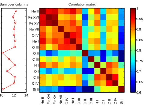
Since our set of 14 lines is partly redundant, some must be eliminated. A well-known measure of redundancy is the cor-relation coefficient, which we compute from the time evolu-tion of the lines. The correlaevolu-tion coefficient between each pair of lines is stored in a correlation matrix defined as
Cφ(λ1, λ2)= 1 T
T
X
t=1
φ (λ1, t )φ (λ2, t )
whereφ (λ, t )is the standardised flux, defined in Sect. 3.2. Cφ(λ1, λ2)is a 14×14 matrix, andλ1andλ2are the wave-lengths of the elements listed in Table 1. The correlation matrix is displayed in Fig. 9. In this example, we look for 6 lines, so 6 classes have to be defined from the correlation matrix, and then one candidate per class must be chosen. A class can be defined as a set of lines that are both highly cor-related to each other and exhibit the same level of correlation to lines that do not belong to that class.
An examination of the correlation matrix suggests the fol-lowing partitioning
cluster 1 He II (30.38 nm) to O III (70.38 nm) cluster 2 O II (83.42 nm)
cluster 3 C III (97.70 nm), H I (121.57 nm) cluster 4 O I (130.43 nm)
Correlation matrix
He II Fe XVI Fe XV Ne VII O IV He I O III O II C III H I O I C II C IV Si II
He II
Fe XVI
Fe XV
Ne VII
O IV
He I
O III
O II
C III
H I
O I
C II
C IV
Si II
0.6 0.65 0.7 0.75 0.8 0.85 0.9 0.95 1
10 12 14
[image:10.595.50.286.59.233.2]Sum over columns
Fig. 9. Correlation matrix of the 14 lines given in Table 1.
Correla-tions lower than 0.6 are marked in dark blue and are not considered to be significant. The degree of correlation of a line with all the other ones is obtained by summing along each row of the correla-tion matrix. This sum is displayed in the left.
For each cluster, we select the line that is the least corre-lated within it (i.e. the least redundant). A simple criterion consists in plotting the sum of the correlation matrix along each row. This sum can be roughly interpreted as the num-ber of elements each line is correlated to; it is plotted on the left of the correlation matrix in Fig. 9. Using this crite-rion, our set of 6 spectral lines becomes: Fe XV (41.76 nm), O II (83.42 nm), H I (121.57 nm), O I (130.43 nm), C II (133.51 nm) and Si II (181.69 nm). This solution is close to the ones we shall derive now, using a more rigourous ap-proach.
4.2 Exhaustive analysis
A more objective selection can be achieved by using a brute force approach, wherein all 3003 combinations of 6 lines out of 14 are compared. For each combination, we estimate the model coefficients by least-squares fitting the channels with a linear combination of the 6 lines, and subsequently com-puting the discrepancy between the original and the mod-elled spectrum. To do so, the samples from which the model is estimated, and those on which the model is subsequently tested, have to be independent. We use the 9 first months of data to estimate the model coefficients, and then test the quality of the fit (i.e. the out-of-sample error) on the remain-ing 13 months. Two natural measures of quality are the sum of squared errors
εa(λ)=
X
t
I (λ, t )−If it(λ, t )
2
and the relative sum of squared errors εr(λ)=
εa(λ)
P
tI (λ, t )2
The former, or absolute error, puts more emphasis on the strongest lines, and is appropriate for total irradiance
mea-20 40 60 80 100 120 140 160 180 200
0 1 2 3 4 5
λ [nm]
relative error
εr
[%]
20 40 60 80 100 120 140 160 180 20010
−7
10−6
10−5
10−4
10−3
10−2
10−1
average flux [W/m
[image:10.595.308.547.65.209.2]2/sec/nm]
Fig. 10. The relative errorεr(λ)(in red) for the best combination of
six lines (see Table 3). The average spectrum (in blue) is shown for comparison, with the six reference spectral lines circled.
surements. It should therefore be preferred for thermospheric applications. Relative errors are better suited for the recon-struction of the shape of the spectrum. The global error is simply the average over all channels. Other measures may also be appropriate, such as a chi-square test, if the number of counts in each channel is known.
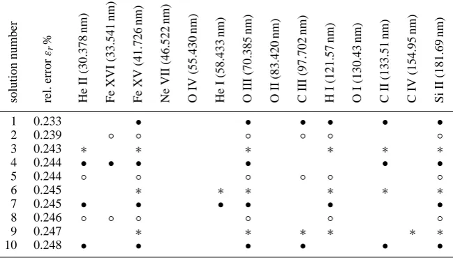
The best combinations of lines turn out to give remark-ably similar errors, whereas the worst combinations are or-ders of magnitude larger. We conclude that there exists a well-determined set of several equally good solutions. The 10 best of them are listed in Table 2 for the absolute errors and in Table 3 for the relative errors.
Not surprisingly, all these combinations involve spectral lines that cover more or less homogeneously the cloud of points in Fig. 5. Absolute errors favour intense (and thus mostly cold) lines, whereas relative errors give priority to a uniform coverage of the spectrum. Some lines definitely stand out, such as the Si II (181.69 nm) line, which describes most of the spectrum from 140 nm onwards. Note that these solutions are very close to the one obtained before by empir-ical correlation analysis.
Clearly, no combination of lines will model all channels equally well. This is illustrated in Fig. 10, which displays the relative error for each channel. The fit is excellent in the least energetic part of the spectrum, which is the easiest to model. The fit gets worse in the vicinity of lines that are most dissimilar to our set, such as Fe XV (28.41 nm) and O VI (103.19 nm). Yet, the relative error on average still remains well below 1%.
Table 2. The 10 best combinations of lines for reconstruction the full EUV spectrum using 6 spectral lines. These combinations minimise
the average absolute error. Each row corresponds to one combination. The errors are expressed in flux units squared. Different symbols are used only to ease reading.
solutio
n
num
ber
abs.
er
ror
εa
×
10
9
He
II
(30.3
78
n
m)
Fe
XV
I
(33
.541
nm)
Fe
XV
(41.7
26
n
m)
N
e
VII
(46.5
22
n
m)
O
IV
(5
5.430
nm)
He
I
(58.
433
nm)
O
II
I
(70.3
85
n
m)
O
II
(83.42
0
nm
)
C
III
(97.702
nm
)
H
I
(12
1.57
nm)
O
I
(130
.43
nm)
C
II
(133
.51
nm)
C
IV
(154
.95
nm)
Si
II
(181.6
9
nm
)
1 1.051 • • • • • •
2 1.076 ◦ ◦ ◦ ◦ ◦ ◦
3 1.078 ∗ ∗ ∗ ∗ ∗ ∗
4 1.095 • • • • • •
5 1.098 ◦ ◦ ◦ ◦ ◦ ◦
6 1.108 ∗ ∗ ∗ ∗ ∗ ∗
7 1.119 • • • • • •
8 1.128 ◦ ◦ ◦ ◦ ◦ ◦
9 1.130 ∗ ∗ ∗ ∗ ∗ ∗
[image:11.595.136.461.352.537.2]10 1.133 • • • • • •
Table 3. Same as Table 2, but with the lines that minimise the average relative error.
solutio
n
num
ber
rel
.
error
εr
%
He
II
(30.3
78
n
m)
Fe
XV
I
(33
.541
nm)
Fe
XV
(41.7
26
n
m)
N
e
VII
(46.5
22
n
m)
O
IV
(5
5.430
nm)
He
I
(58.
433
nm)
O
II
I
(70.3
85
n
m)
O
II
(83.42
0
nm
)
C
III
(97.702
nm
)
H
I
(12
1.57
nm)
O
I
(130
.43
nm)
C
II
(133
.51
nm)
C
IV
(154
.95
nm)
Si
II
(181.6
9
nm
)
1 0.233 • • • • • •
2 0.239 ◦ ◦ ◦ ◦ ◦ ◦
3 0.243 ∗ ∗ ∗ ∗ ∗ ∗
4 0.244 • • • • • •
5 0.244 ◦ ◦ ◦ ◦ ◦ ◦
6 0.245 ∗ ∗ ∗ ∗ ∗ ∗
7 0.245 • • • • • •
8 0.246 ◦ ◦ ◦ ◦ ◦ ◦
9 0.247 ∗ ∗ ∗ ∗ ∗ ∗
10 0.248 • • • • • •
model accurately. As will be shown now, adding more lines does not necessarily improve these results.
5 Best solutions for 1 up to 10 spectral lines
To conclude this study, we consider the best combinations of 1 up to 10 spectral lines. The solutions that minimise the absolute error are listed in Table 4. Some elements are better than others. Two examples are the Si II (181.69 nm) and the Fe XV (41.73 nm) lines, which describe two extremes of the spectral variability. The strong H I (121.57 nm) line stands out because it happens to describe a large cluster of channels. Let us stress again that these selections are context dependent and may change, for example, if a smaller fraction
of the spectrum needs to be reconstructed or if a flare must be rendered.
Table 4. The 3 best combinations for reconstruction the full EUV spectrum using 1 up to 10 spectral lines. These solutions minimise the
absolute error.
n
umber
of
lin
es
H
e
II
(3
0.378
nm)
Fe
XVI
(33.54
1
nm
)
Fe
XV
(4
1.726
nm)
Ne
V
II
(46
.522
nm)
O
IV
(55.43
0
nm
)
He
I
(5
8.433
nm)
O
III
(7
0.385
nm
)
O
II
(83
.420
nm)
C
III
(97
.702
nm)
H
I
(121.5
7
nm
)
O
I
(1
30.43
nm
)
C
II
(1
33.51
nm)
C
IV
(154.95
nm
)
S
i
II
(18
1.69
nm)
•
1 ◦
∗
• •
2 ◦ ◦
∗ ∗
• • •
3 ◦ ◦ ◦
∗ ∗ ∗
• • • •
4 ◦ ◦ ◦ ◦
∗ ∗ ∗ ∗
• • • • •
5 ◦ ◦ ◦ ◦ ◦
∗ ∗ ∗ ∗ ∗
• • • • • •
6 ◦ ◦ ◦ ◦ ◦ ◦
∗ ∗ ∗ ∗ ∗ ∗
• • • • • • •
7 ◦ ◦ ◦ ◦ ◦ ◦ ◦
∗ ∗ ∗ ∗ ∗ ∗ ∗
• • • • • • • •
8 ◦ ◦ ◦ ◦ ◦ ◦ ◦ ◦
∗ ∗ ∗ ∗ ∗ ∗ ∗ ∗
• • • • • • • • •
9 ◦ ◦ ◦ ◦ ◦ ◦ ◦ ◦ ◦
∗ ∗ ∗ ∗ ∗ ∗ ∗ ∗ ∗
• • • • • • • • • •
10 ◦ ◦ ◦ ◦ ◦ ◦ ◦ ◦ ◦ ◦
∗ ∗ ∗ ∗ ∗ ∗ ∗ ∗ ∗ ∗
lines will cause overfitting: either the model is trying to fit the statistical variability that is inherent in any photon counting process, or the model misses some fine deterministic effects. Although the shape of the minimum may slightly change as longer time series become available, we can safely conclude that the optimum number of spectral lines is between 5 and 8. This justifies a posteriori our previous choice of 6 lines in Sect. 4 and supports the conclusions of Kretzschmar et al. (2005).
It is interesting to compare these results with reconstruc-tions achieved using proxies only. We already know from Fig. 6 that the Mg II index is a good proxy for the UV spectrum above 140 nm, whereas F10.7 and E10.7 are better suited for more energetic lines. The smallest errors are ob-tained with a combination of the Mg II and F10.7 (or E10.7) indices. These errors, however, still exceed by almost one order of magnitude those obtained using a pair of spectral lines, see Fig. 12. A good combination of two or more spec-tral lines therefore is always preferable to any combination of proxies.
All these results are of course open to improvement and additional constraints can be added to the procedure. We
have deliberately avoided technical issues that may become important once the model has to be tailored to specific needs. One of these issues is the departure from a linear model. The fitting capacity of our model can be expanded by including combinations of nonlinear functions of the fluxes, but this will also dramatically increase the need for careful model validation. We did try some of these alternatives (see Nelles, 2001, for a survey of methods), considering for example lin-ear combinations of the fluxes and their values squared. No significant improvement, however, was observed.
6 Conclusions
The aim of this study is to answer the following questions: – If we want to reconstruct the full EUV spectrum
be-tween 26 and 194 nm from a linear combination of a few calibrated spectral lines, how many lines should we measure?
2002 2003 2004 2005 −0.5
0 0.5
amplitude vs mean value
year
Fe XV
Ne VII
He II
C I
28.41 nm
46.52 nm
30.38 nm
[image:13.595.311.547.59.219.2]156.10 nm measured modelled
Fig. 11. Comparison between the measured (blue and dashed) and
the fitted (red) flux, for 4 typical spectral lines. The fit is based on the 6 lines that minimise the absolute error. The model param-eters are estimated from the first 9 months (area shown in grey); the quality of the fit should therefore not be considered inside this interval. Note that the Fe XV channel shows degradations starting early 2004; these are not taken into account in the computation of the error criterion.
In contrast to previous studies, we consider an empirical and data-driven approach, which is based on two years of TIMED/SEE irradiance measurements. Our study first shows that all spectral lines can be conveniently represented on a 2-D map according to the similarities in their temporal evo-lution. From this, we extract a first set of 14 intense lines that are representative of the full spectrum. Next, we show that a subset of 5 to 8 of these lines is sufficient for reconstruct-ing the spectrum with a relative error below 0.25%. The best solutions are context dependent: a minimisation of the total irradiance error does not lead to the same set of lines as the minimisation of the relative error. For that reason we focus on the methodology rather than on the solutions themselves. Such spectral reconstructions show a significant improve-ment over results achieved with proxies only, such as the F10.7 index. Our 2-D representation is convenient for show-ing why proxies fail in reproducshow-ing some parts of the spectral variability. It also reveals which spectral lines could reason-ably be fitted by a combination of proxies.
This work is open to several improvements. Repeating it on longer time series, hopefully extending through solar minimum, is of course a priority. The contribution of solar flares, which has been excluded so far, is expected to enrich the spectral dynamics, probably giving rise to a different 2-D representation for each particular flare. One can also ap-ply the same statistical approach to the continuum only. The stronger redundancy of the latter results in a smaller set of lines. Finally, the multidimensional scaling technique can be extended to include nonlinear mappings (for example self-organised maps) or multiscale decompositions.
1 2 3 4 5 6 7 8 9 10 11 12 13 14 0
0.5 1 1.5 2
number of spectral lines
error
ε
proxy
absolute error * 108 relative error [%]
Fig. 12. The minimum error (absolute and relative) achieved with
the best combination of 1 up to 14 lines. Also shown (on the far right), are the errors obtained by fitting the spectrum using the two best proxies (Mg II index and F10.7 index).
Most important of all, this study paves the way for a new methodology for selecting the spectral lines that best capture the salient features of the spectral variability in the EUV do-main. Because the method is data-driven, it is arguably more appropriate for selecting those lines. It is also a powerful tool for instrument definition and specification. In particular, a spectral reconstruction based on a series of measurements with different passbands (e.g. from radiometers) is possible.
Appendix A: the Singular Value Decomposition
The Singular Value Decomposition (SVD) is a fundamental tool in linear algebra (Press et al., 1992) and in statistical analysis (Chatfield and Collins, 1990). In addition to that, it has several interpretations and some remarkable properties. LetI (λ, t )denote the solar flux at timetand wavelengthλ. Since the flux exhibits a similar time evolution at different wavelengths, one may assume that the whole spectrum be-haves like a single time seriesg1(t )that is weighted by the intensity at each wavelength. We therefore look for variables g1(t )andf1(λ)such that
I (λ, t )=f1(λ)g1(t )+ε1,
where ε is some residual error to be minimised in a least-squares sense. The variablesf andgcan be uniquely deter-mined, provided they are normalised. Let us normalise them in the following way
hf1(λ)f1(λ)i = hg1(t )g1(t )i =1,
whereh· · ·i denotes averaging over the corresponding vari-able. One then needs to introduce a weightW1, so that I (λ, t )=W1f1(λ)g1(t )+ε1.
Not all spectral lines may exhibit the same time evolution, so we add a first order correction, which must also be a separa-ble function of time and wavelength
[image:13.595.50.288.63.248.2]