Comparison of robustness to outliers between robust poisson models and log-binomial models when estimating relative risks for common binary outcomes: a simulation study

(1)

R E S E A R C H A R T I C L E

Open Access

Comparison of robustness to outliers between

robust poisson models and log-binomial models

when estimating relative risks for common binary

outcomes: a simulation study

Wansu Chen

1,2*

, Jiaxiao Shi

1

, Lei Qian

1

and Stanley P Azen

2

Abstract

Background:To estimate relative risks or risk ratios for common binary outcomes, the most popular model-based methods are the robust (also known as modified) Poisson and the log-binomial regression. Of the two methods, it is believed that the log-binomial regression yields more efficient estimators because it is maximum likelihood based, while the robust Poisson model may be less affected by outliers. Evidence to support the robustness of robust Poisson models in comparison with log-binomial models is very limited.

Methods:In this study a simulation was conducted to evaluate the performance of the two methods in several scenarios where outliers existed.

Results:The findings indicate that for data coming from a population where the relationship between the outcome and the covariate was in a simple form (e.g. log-linear), the two models yielded comparable biases and mean square errors. However, if the true relationship contained a higher order term, the robust Poisson models consistently outperformed the log-binomial models even when the level of contamination is low.

Conclusions:The robust Poisson models are more robust (or less sensitive) to outliers compared to the log-binomial models when estimating relative risks or risk ratios for common binary outcomes. Users should be aware of the limitations when choosing appropriate models to estimate relative risks or risk ratios.

Keywords: Relative risk, Risk ratio, Log-binomial regression, Robust poisson regression, Outliers, Common binary outcomes

Background

When the outcome of a study is binary, the most com-mon method to estimate the effect is to calculate an odds ratio (OR) as an estimate of relative risk (RR) using a logistic regression. When the outcome prevalence is high (>10%), the OR can still be estimated by using the logistic regression model, but the OR is no longer an ac-ceptable estimate for RR [1]. Interpreting the OR as be-ing equivalent to the RR still occurs in medical research, leading to overstated effect in the study findings [2,3].

The degree of overstatement depends on the outcome rate (e.g., disease prevalence). A higher outcome rate leads to higher degree of exaggeration. Zhang and Yu proposed a formula to convert the adjusted OR derived from the logistic regression model to a risk ratio in studies with common outcomes [4]. However, the method was noted by McNutt et al. to produce biases in both point es-timates and confidence intervals (CIs) [5]. Miettinen sug-gested the doubling-of-cases method to estimate OR as an approximation of RR using logistic regression based on a modified dataset [6]. Schouten et al. improved the method by applying robust standard errors [7]. However, this method was mentioned by Skov et al. to produce preva-lence greater than one [8]. Several model-based methods have been proposed to estimate RR and its CI directly [9]. * Correspondence:[email protected]

1_{Kaiser Permanente Southern California, Department of Research and}

Evaluation, Pasadena, CA, USA

2_{Department of Preventive Medicine, Keck School of Medicine, University of}

Southern California, Los Angeles, CA, USA

(2)

The most popular ones are the robust (also known as modified) Poisson model [10-12] and the log-binomial model [8,11,13]. The performance based on simulations seemed to be equally good between the log-binomial model and the robust Poisson model [3,11,12,14] when sample sizes are reasonably large. Out of the two models, it was reported that the robust Poisson may be less af-fected by outliers compared to the log-binomial method [15]. However, the research in this area is very limited. The purpose of this study is to evaluate the performance of the two methods using simulation in several scenarios when outliers exist and to provide insight into the selec-tion of the appropriate models.

Methods

Estimation methods

The Poisson regression uses a logarithm as the natural link function under the generalized linear model framework. When the outcome is common, the standard Poisson re-gression over estimates the variance for the measured ef-fect [10-12]. The robust Poisson regression model uses the classical sandwich estimator under the generalized estima-tion equaestima-tion (GEE) framework to correct the inflated vari-ance (also known as over-dispersion) in the standard Poisson regression. This correction can be achieved by using the REPEATED statement in SAS Proc GENMOD [12] or the ROBUST option in STATA’s Poisson procedure [11]. The estimators based on the robust Poisson models are pseudo-likelihood estimators.

The log-binomial regression approach models the prob-ability of having the outcome (e.g., disease) based on the binomial distribution and logrithm of the probability as the link function in a generalized linear model [8,13]. The log-binomial model attempts to find a MLE if it exists. MLEs are preferred estimators because they carry many good properties including higher efficiency compared to non-MLE estimators. The analyses can be performed using SAS’s GENMOD, R’s GLM or STATA’s GLM pro-cedure. However, for many situations in which quantita-tive covariates exist, the MLE can be on the boundary of the parameter space (i.e. the predicted probability of the outcome equals to 1), leading to the difficulty of finding the MLE. To address the non-convergence issue, a SAS macro called “COPY” was developed [16] and later en-hanced [17] to increase the chance of finding an approxi-mate MLE inside the interior of the parameter space using PROC GENMOD. The COPY method uses the results of the log-binomial regression if the model converges. When the log-binomial regression fails to converge, the COPY method creates C (usually a large number) copies of the original data and one copy of the original data with the outcome variable reversed (Y converted to 1-Y) and then takes the modified data to generate the estimates [16]. The enhanced version of the COPY method simply

generated virtual copies by applying weights of C and 1, re-spectively, to the original dataset and the dataset with the outcome variable reversed [17]. The choice of C impacts the accuracy and the efficiency of the estimates as well as the model convergence. A larger C produces results that are closer to MLEs yet leads to a higher level of difficulty in finding the MLEs due to failure of convergence [17].

Simulation methods

Design of uncontaminated datasets

LetXbe a binary treatment/exposure variable (X= 1 for

treatment/exposure and X= 0 for

non-treatment/non-exposure) from a binomial distribution with the prob-ability of X= 1 fixed at 50%. Let Ybe a binary common outcome from a population with the probability ofY= 1

varying from 10%, 25% to 40%. Let Z be a continuous

confounder following the Beta (6, 2) distribution. The Beta distribution offers a wide range of possible forms. The parameters chosen (α= 6 and β= 2) provided the distribution with a mean of approximately 0.75. If Z× 100 represents the ages of study subjects, they came from an elderly population with the average age being 75 years old. The relationship between X and Z is de-fined by the equation logit (px) =a0+a1Z, wherea1= log (2) or log (4) to indicate moderate or strong association, respectively. The relationship between Yand X is log-linear with adjustedRRbeing 1.5 or 2.Zis designed as a linear or quadratic confounder.

Linear cofounder Z: logð Þ ¼p_v β0þβ1Xþβ2Z; or

Quadratic cofounder Z: logð Þ ¼p_v β0þβ1Xþβ2Z

þð0:5β₂ÞZ2_;

where β₁¼ log 1ð Þ:5 or log 2ð Þ;and β₂¼ log 2ð Þor log 4ð Þ

The value of β1in the models denotes the effect due to exposure on the log-relative risk scale (i.e. β1= log (RR)). To simplify the design, we setβ2=α1. There were a total of 24 scenarios (2 RRs, 3 outcomes, 2 levels of as-sociation, 2 types of confounders). A detailed description of the 24 scenarios is listed in“Additional file 1”.

Data generating process

(3)

moderate sizes, the same process was repeated to generate another set of data with n = 500.

Contaminating the datasets

For each of the 24 scenarios, the simulation datasets were contaminated by flipping the outcomes (Ybecomes 1-Y) of the records that had the extreme probabilities of having Y= 1 (i.e., either very low or very highpy). Models were assessed by using the original simulated datasets and the datasets contaminated at the following level.

Contamination rates:

0%–original datasets

2%–flipping the outcomes of records withpyat bottom or top 1%

5%–flipping the outcomes of records withpyat bottom or top 2.5%

Although it is not realistic to expect outliers to solely come from observations with very low or very high probabilities of having the outcome, outliers resulting from flipping the outcome are possible due to documen-tation or data entry errors. For example,“0”(“not having

the disease”) may be erroneously entered into the study database as“1”(“the disease was present”). Compared to adding outliers from a distribution that is different from the underlying one, the flipping approach produced out-liers that are more likely to be leverage points. In other words, they are more likely to impact the estimates.

Measures of model performance

For each scenario, the simulation process was repeated 1,000 times to estimate the relative bias, standard error and mean square error (MSE) for the log-binomial model and the robust Poisson model. The relative bias was calcu-lated as the average of the 1,000 estimated RR in log scale minus the log of the true RR divided by the log of the true RR. Standard error was defined as the empirical standard error of the estimated RR in log scale over all 1,000 simu-lations. MSE was calculated by taking the sum of the squared bias in log scale and the variances.

Due to the non-convergence issue in standard statis-tical software, we used the COPY method to generate the estimates of the log-binomial models. However, the accuracy of parameter estimates depends on the number of virtual copies. For this evaluation the number of copies

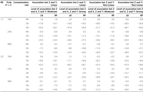
Table 1 Relative bias (%) in log scale (n = 1500)

RR Prob (Y = 1)

Contamination rate

Association bet Z and Y: Linear

Association bet Z and Y: Non-Linear

Level of association bet Z and X, Z and Y: Moderate

Level of association bet Z and X, Z and Y: Strong

LB RP LB RP LB RP LB RP

1.5 10% 0% 1.8 1.8 2.0 2.0 0.0 0.0 −0.6 −0.8

2% −17.8 −16.7 −16.0 −16.0 −30.0 −19.5 −28.5 −20.4

5% −43.4 −36.7 −41.8 −36.9 −51.7 −41.3 −49.1 −43.0

25% 0% −0.4 −0.4 0.4 0.3 0.5 0.5 −0.8 −0.8

2% −10.4 −10.9 −10.1 −11.4 −14.1 −11.8 −18.6 −16.2

5% −25.3 −24.4 −26.6 −27.3 −34.6 −28.2 −43.4 −36.2

40% 0% 0.2 0.2 −0.7 −0.7 −0.0 −0.1 0.9 0.7

2% −7.5 −8.0 −9.8 −10.8 −11.0 −10.5 −14.9 −13.1

5% −19.2 −19.4 −23.4 −24.6 −26.9 −24.7 −36.9 −32.2

2.0 10% 0% 0.4 0.4 1.5 1.5 −0.2 −0.2 0.6 0.7

2% −18.9 −18.1 −17.1 −16.8 −26.3 −19.0 −25.0 −18.0

5% −42.0 −37.5 −40.2 −36.7 −47.9 −39.5 −47.4 −39.6

25% 0% 0.5 0.5 0.3 0.3 0.3 0.3 0.9 0.8

2% −9.0 −9.2 −9.2 −9.9 −12.3 −10.4 −13.7 −11.7

5% −23.3 −22.2 −23.7 −23.6 −30.0 −24.7 −34.5 −28.5

40% 0% −0.1 −0.1 0.1 0.1 0.3 0.3 −0.3 −0.3

2% −6.7 −7.0 −7.2 −7.8 −8.4 −8.0 −10.9 −10.2

5% −16.9 −16.6 −18.5 −19.0 −21.2 −19.5 −26.6 −24.5

Association between Z and X always linear. LB: Log-Binomial Model.

RP: Robust Poisson.

(4)

were set to 1,000,000, the default of the COPY method [17]. All the datasets were generated and analyzed using SAS Version 9.2 [18].

Results Relative bias

Table 1 and Figure 1 revealed the relative biases of the estimated RR in log scale from the two models in each of the 24 scenarios mentioned above when n = 1,500. As expected, both models accurately estimated β1 or log (RR) when the simulated databases were not contami-nated (level of contamination = 0%). When the data were contaminated (level of contamination > 0%), the relative biases were all negative, indicating that the point esti-mates were biased towards null. For a fixed RR and an outcome rate, the absolute value of the relative biases in-creased quickly with the level of contamination. How-ever, the pace of such an increase varied by the outcome

rate. Scenarios with lower outcome rates seemed to be associated with more elevated absolute relative biases.

Models with linear confounder Z

When the models contained a linear confounder Z, the two models yielded comparable relative biases (Table 1, Figures 1A and B) except for a few scenarios in which the biases from the log-binomial models were slightly larger than those of the robust Poisson models. The lar-gest differences occurred when the contamination rate was 5% and the outcome rate was 10%, in which the log-binomial models had 3.5%-6.7% higher biases compared to the corresponding robust Poisson models.

Models with non-linear confounder Z

With the non-linear confounder Z, the robust Poisson model outperformed the log-binomial model when the data was contaminated (Table 1, Figure 1C and D). The

(5)

difference between the two models was visible even when the level of contamination was only 2%. The mag-nitude of difference between the two models also varied with the outcome rate. A larger difference was associ-ated with smaller outcomes.

Standard Error (SE)

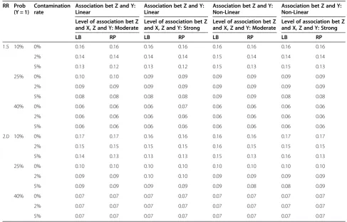
When the simulated databases were not contaminated (level of contamination = 0%), the SEs of the two models were identical at the 2nd decimal point (Table 2). When the levels of contamination were greater than 0%, the es-timated SEs remained comparable between the two models when the outcome rates were high (25% or 40%). However, when the outcome rate was low (10%), the SEs derived from the log-binomial models seemed to be slightly higher than those of robust Poisson in some of the scenarios.

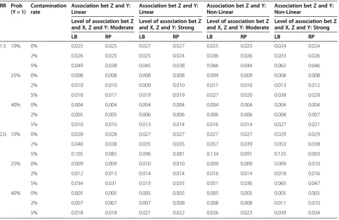
Mean Square Error (MSE)

The same pattern was observed for the MSEs as those of relative biases (Table 3). When the models contained a linear confounder Z, the two models had comparable

MSEs except when the outcome rate was 10% and the contamination reached 5%. When the models contained a non-linear confounder Z, the two models diverged even when the degree of contamination was only 2% (Table 3).

When the simulation was conducted based on samples of moderate sizes (n = 500), the same pattern was ob-served. As expected, the SEs based on the small samples were larger compared to those derived from large sam-ples (n = 1,500). The results summarized from samsam-ples of size 500 were included in“Additional file 2”.

Discussion

In this study, evaluation was performed on the statistical properties of the two most popular model-based ap-proaches to estimate RR for common binary outcomes in various scenarios when outliers existed. The results suggest that for data coming from a population in which the true relationship between the outcome and the covariate is not in a simple form (e.g., containing a higher order term), the robust Poisson model consist-ently outperforms the log-binomial model even when the level of contamination is low (e.g., 2%). Statistical

Table 2 Standard error in log scale (n = 1500)

RR Prob (Y = 1)

Contamination rate

1.5 10% 0% 0.16 0.16 0.16 0.16 0.16 0.16 0.16 0.16

2% 0.14 0.14 0.14 0.14 0.15 0.14 0.14 0.14

5% 0.13 0.12 0.13 0.12 0.15 0.13 0.15 0.13

25% 0% 0.10 0.10 0.09 0.09 0.09 0.09 0.09 0.09

2% 0.09 0.09 0.09 0.09 0.09 0.09 0.09 0.09

5% 0.08 0.08 0.08 0.08 0.09 0.09 0.08 0.08

40% 0% 0.06 0.06 0.06 0.07 0.06 0.06 0.06 0.06

2% 0.06 0.06 0.06 0.06 0.06 0.06 0.06 0.06

5% 0.06 0.06 0.06 0.06 0.06 0.06 0.06 0.06

2.0 10% 0% 0.17 0.17 0.16 0.16 0.16 0.16 0.17 0.17

2% 0.15 0.15 0.15 0.15 0.16 0.15 0.15 0.15

5% 0.14 0.13 0.13 0.13 0.15 0.13 0.16 0.13

25% 0% 0.10 0.10 0.10 0.10 0.10 0.10 0.10 0.10

2% 0.09 0.09 0.10 0.10 0.09 0.09 0.09 0.09

5% 0.09 0.09 0.09 0.09 0.09 0.08 0.08 0.09

40% 0% 0.07 0.07 0.07 0.07 0.07 0.07 0.07 0.07

2% 0.07 0.07 0.07 0.07 0.07 0.07 0.07 0.07

5% 0.07 0.07 0.07 0.07 0.07 0.07 0.07 0.07

RP: Robust Poisson.

(6)

software utilizes iterative weighted least squares (IWLS) approach or variations of IWLS to find MLEs for general-ized linear models. For log-binomial models, the weights used by the IWLS approach contain the term 1/(1-p), wherep= exp (XTβ) with a range from 0 to 1 [19]. Lumley et al. pointed out that the MLE of a log-binomial model is likely to be too sensitive to outliers because a very large p (referred to asμby the authors) has a large influ-ence on the weights, even though the sum of the covariate values are still bounded [15]. In our study both the MLE, generated by the log-binomial models and the pseudo-likelihood estimators, produced by the robust Poisson models, were deteriorated when outliers were introduced. However, the level of deterioration differed when the rela-tionships between the confounder and the outcome was not in a simple form, possibly due to the bigger “μ”s yielded by the log-binomial model when the higher-order term ofZwas added into the model.

Deddens and Pertersen compared the log-binomial and robust Poisson models by using three real-life examples [20]. Out of the three examples, two produced different point estimates and SEs. In one of these two examples, the difference was nearly two folds for both point estimates

and SEs for one of the covariates. The authors concluded that“the decision on which method to use is very import-ant”[20]; however, since the truth was unknown, it is un-likely to tell that between the log-binomial model and the robust Poisson model, which one can yield estimates that are closer to the truth. In one of the two examples in which differences between the two models were observed, the model contained a higher-order (quadratic) term. It is unclear whether or not the complexity of the model degen-erated the performance of the models, especially for the log-binomial model.

Of the two methods, the log-binomial method is generally preferred due to the fact that the MLEs esti-mated by the log-binomial models are more efficient compared to the pseudo-likelihood estimators used by the robust Poisson models ([10], page 2300). Spiegelman and Hertzmark recommend using the log-binomial models over the robust Poisson models when convergence is not an issue [21]. Very small differences were observed in a simulation study with a sample size of 100 and a single independent variable with a uniform distribution [14]. When data perfectly follows a log-binomial distribution (i.e., without outliers), the current study did not observe

Table 3 Mean Square Error (MSE) in log scale (n = 1500)

RR Prob (Y = 1)

Contamination rate

1.5 10% 0% 0.025 0.025 0.027 0.027 0.025 0.025 0.024 0.024

2% 0.026 0.025 0.025 0.024 0.036 0.026 0.033 0.026

5% 0.049 0.038 0.045 0.038 0.066 0.044 0.063 0.046

25% 0% 0.008 0.008 0.008 0.008 0.009 0.009 0.008 0.008

2% 0.010 0.010 0.009 0.010 0.011 0.010 0.013 0.012

5% 0.018 0.017 0.019 0.019 0.027 0.020 0.038 0.028

40% 0% 0.004 0.004 0.004 0.004 0.004 0.004 0.004 0.004

2% 0.005 0.005 0.006 0.006 0.006 0.006 0.008 0.007

5% 0.010 0.010 0.013 0.014 0.016 0.014 0.027 0.021

2.0 10% 0% 0.028 0.028 0.027 0.027 0.027 0.027 0.029 0.029

2% 0.040 0.038 0.035 0.035 0.057 0.039 0.053 0.038

5% 0.105 0.085 0.096 0.081 0.134 0.091 0.135 0.093

25% 0% 0.009 0.009 0.010 0.010 0.009 0.009 0.009 0.010

2% 0.012 0.013 0.014 0.014 0.016 0.014 0.018 0.016

5% 0.034 0.031 0.013 0.035 0.051 0.036 0.065 0.047

40% 0% 0.005 0.005 0.005 0.005 0.005 0.005 0.005 0.005

2% 0.007 0.007 0.007 0.008 0.008 0.008 0.011 0.010

5% 0.018 0.018 0.021 0.022 0.026 0.023 0.039 0.034

RP: Robust Poisson.

(7)

any difference in either biases or variances between the log-binomial and the robust Poisson models for large (n = 1,500) and moderate (n = 500) sample sizes. It appears that the gain in efficiency is beneficial to log-binomial models only for samples of small sizes.

It is not a surprise to observe negative biases when the simulation datasets were contaminated, because flipping the outcomes of the records that have the very low or very high probabilities tend to weaken the associations between the exposure and the outcome leading the asso-ciations towards null. The observation of more elevated biases when outcome rate = 10% compared to those of 25% and 40% comes with no surprise either since the impact of flipping on the estimates is expected to be more significant for scenarios with more extreme out-comes (close to 0% or 100%).

Robust methods to detect outliers especially high le-verage points for logistic regression models are available in popular statistical software packages [22-24]. How-ever, similar approaches for log-binomial models are not yet available in commercial software packages although the adoption of the diagnostic statistics from those of lo-gistic regression models were demonstrated and applied in a real life example [25]. Efforts to develop goodness of fit tests resulted in reasonable type I errors yet low to moderate power [25]. For this reason, the robust Poisson model seems to be a more attractive choice due to its capability of providing more robust results when outliers are undetected.

For the COPY method, the accuracy of parameter esti-mates depends on the number of virtual copies. Peterson and Deddens pointed out that“with 10,000 copies the re-sults were generally accurate to three decimal places” in their scenarios [17]. Therefore, the number of virtual cop-ies we used (1,000,000) should provide accuraccop-ies that are high enough for our evaluation. The number of virtual copies should be carefully chosen, because a high number of virtual copies may result in failure of convergence.

Occasionally, failure of convergence remains to be an issue for log-binomial models even if the COPY method is applied. Peterson and Deddens [14] included a con-tinuous exposure variable (referred to as the concon-tinuous covariate by the authors) when applying the COPY method in the simulation and reported a range of con-vergence between 70% and 100%. In this study where C, the number of the virtue copies, was set to be 1,000,000, the COPY method converged in all 1,000 simulations in all the 48 scenarios with the linear confounder, and in 30 of out 48 scenarios with the non-linear confounder. In the 18 scenarios in which the COPY method did not converge in all 1,000 simulations (failed in 1 or more simulations), the converge rates ranged from 0.983 to 0.999 (median 0.996). If the COPY method fails to con-verge and the maximum likelihood-based estimators are

desired, one can choose the Non-Linear Programming (NLP) procedure in SAS [26]. The NLP method is compu-tationally expensive. However, it does not encounter any convergence issues.

Given the lack of robustness of log-binomial models, the authors recommend using robust Poisson models to estimate RR when there are continuous covariates in the model, especially when the covariates are not in a simple linear form. Due to the concern of lack of ef-ficiency for the robust Poisson models for small samples, log-binomial may still be the choice when the sample size is small.

A potential limitation of this study is that complex forms between the confounder and the outcome were generated by a quadratic equation. It is not clear whether or not the findings can be generalized to other complex situations. In addition, all of the outliers generated oc-curred to records with very low or very high probabilities and such outliers are more likely to be leverage points. The impact of the outliers generated by this study could be more significant compared to that of another study with outliers that were differently distributed.

In summary, the current study revealed the evidence to support the robustness of the robust Poisson model in various scenarios. Further research should focus on the model misspecification due to deviations of under-lying probabilities. It is desirable for future studies to de-velop methods to identify leverage points and efficient goodness-of-fit test for log-binomial models.

Conclusions

The robust Poisson models are more robust to outliers compared to the log-binomial models when estimating relative risks or risk ratios for common binary outcomes. Users should be aware of the limitations when choos-ing appropriate models to estimate relative risks or risk ratios.

Additional files

Additional file 1:Description of 24 Scenarios for Data Generation.

Additional file 2:Relative Bias (%), Standard Error (SE) and Mean Square Error (MSE) When n = 500.

Abbreviations

OR:Odds ratio; RR: Relative risk; MLE: Maximum likelihood estimator; GEE: Generalized estimation equation; SE: Standard error; MSE: Mean square error.

Competing interests

The authors declare that they have no competing interests.

Authors’contributions

(8)

analyses. SA participated in the design and provided guidance. All the authors read and approved the final manuscript.

Acknowledgements

We would like to thank Bonnie Li, M.S. for the programming assistance.

Received: 27 February 2014 Accepted: 19 June 2014 Published: 26 June 2014

References

1. Greenland S:Interpretation and choice of effect measures in epidemiologic analyses.Am J Epidemiol1987,125(5):761–768.

2. Agrawal D:Inappropriate interpretation of the odds ratio: oddly not that uncommon.Pediatrics2005,116:1612–1613.

3. Mirjam JK, Cessie SL, Algra A, Vandenbroucke JP:Overestimation of risk ratios by odds ratios in trials and cohort studies: alternatives to logistic regression.Can Med Assoc J2012,184(8):895_–899.

4. Zhang J, Yu KF:What’s relative risk? A method of correcting the odds ratio in cohort studies of common outcomes.JAMA1998, 280:1690–1691.

5. McNutt LA, Wu C, Xue X, Hafner JP:Estimating the relative risk in cohort studies and clinical trials of common outcomes.Am J Epidemiol2003, 157(10):940–943.

6. Miettinen O:Design options in epidemiologic research. An update.Scand J Work Environ Health1982,8(Suppl 1):7–14.

7. Schouten EG, Dekker JM, Kok FJ, Le Cessie S, Van Houwelingen HC, Pool J, Vanderbroucke JP:Risk ratio and rate ratio estimation in case-cohort designs: hypertension and cardiovascular mortality.Stat Med1993, 12:1733–1745.

8. Skov T, Deddens J, Petersen MR, Endahl L:Prevalence proportion ratios: estimation and hypothesis testing.Int J Epidemiol1998, 27:91–95.

9. Greenland S:Model-based estimation of relative risks and other epidemiologic measures in studies of common outcomes and in case_–control studies.Am J Epidemiol2004,160(4):301_–305. 10. Stijnen T, Van Houwelingen HC:Relative risk, risk difference and rate

difference models for sparse stratified data: a pseudo likelihood approach.Stat Med1993,12(24):2285–2303.

11. Barros AJ, Hirakata VN:Alternatives for logistic regression in cross-sectional studies- an empirical comparison of models that directly estimate the prevalence ratio.BMC Med Res Method2003,3(21):1–13.

12. Zou G:A modified poisson regression approach to prospective studies with binary data.Am J Epidemiol2004,159(7):702–706.

13. Wacholder S:Binomial regression in GLIM: estimating risk ratios and risk differences.Am J Epidemiol1986,123:174–184.

14. Petersen MR, Deddens JA:A comparison of two methods for estimating prevalence ratios.BMC Med Res Method2008,8(1):9.

15. Lumley T, Kronmal RA, Ma S:Relative risk regression in medical research: models, contrasts, estimators and algorithms. UW Biostatistics Working Paper Series 293.Seattle, WA: University of Washington; http://www.bepress.com/ uwbiostat/paper293. Accessed June 20, 2014.

16. Deddens JA, Petersen MR, Lei X:Estimation of Prevalence Ratios When PROC GENMOD Does not Converge, In Proceedings at the SAS Users Group International Proceedings: March 30 SUGI28. Washington: Seattle; 2003.

17. Petersen MR, Deddens JA:A revised SAS macro for maximum likelihood estimation of prevalence ratios using the COPY method [letter].

Occup Environ Med2009,66(9):639.

18. Institute SAS:Software Version 9.2.Cary, North Carolina: SAS Institute; 2008. 19. McCullagh P, Nelder J:Generalized Linear Models.Secondthth edition. New

York: John Wiley & Sons; 1989.

20. Deddens JA, Petersen MR:Approaches for estimating prevalence ratios.

Occup Environ Med2008,65:501–506.

21. Spiegelman D, Hertzmark E:Easy SAS calculations for risk or prevalence ratios and differences.Am J Epidemiol2005,162:199–200.

22. Hosmer DW, Lemeshow S:Applied Logistic Regression.2nd edition. New York: John Wiley & Sons; 2000.

23. Imon AHMR, Hadi AS:Identification of multiple high leverage points in logistic regression.J Appl Stat2013,40(12):2601–2616.

24. Syaiba BA, Habshah M:Robust logistic diagnostic for the identification of high leverage points in logistic regression model.J Appl Sci2010, 10(23):2042–3050.

25. Blizzard L, Hosmer DW:Parameter estimation and goodness-of-fit in log binomial regression.Biometrical J2006,48(1):5–22.

26. Yu B, Wang Z:Estimating relative risks for common outcome using PROC NLP.Comput Meth Prog Bio2008,90(2):179–186.

doi:10.1186/1471-2288-14-82

Cite this article as:Chenet al.:Comparison of robustness to outliers between robust poisson models and log-binomial models when estimating relative risks for common binary outcomes: a simulation study.BMC Medical Research Methodology201414:82.

Submit your next manuscript to BioMed Central and take full advantage of:

• Convenient online submission

• Thorough peer review

• No space constraints or color ﬁgure charges

• Immediate publication on acceptance

• Inclusion in PubMed, CAS, Scopus and Google Scholar

• Research which is freely available for redistribution