R E S E A R C H A R T I C L E
Open Access
Reliability in evaluator-based tests: using
simulation-constructed models to
determine contextually relevant agreement
thresholds
Dylan T. Beckler, Zachary C. Thumser, Jonathon S. Schofield and Paul D. Marasco
*Abstract
Background:Indices of inter-evaluator reliability are used in many fields such as computational linguistics, psychology, and medical science; however, the interpretation of resulting values and determination of appropriate thresholds lack context and are often guided only by arbitrary“rules of thumb”or simply not addressed at all. Our goal for this work was to develop a method for determining the relationship between inter-evaluator agreement and error to facilitate meaningful interpretation of values, thresholds, and reliability.
Methods:Three expert human evaluators completed a video analysis task, and averaged their results together to create a reference dataset of 300 time measurements. We simulated unique combinations of systematic error and random error onto the reference dataset to generate 4900 new hypothetical evaluators (each with 300 time measurements). The systematic errors and random errors made by the hypothetical evaluator population were approximated as the mean and variance of a normally-distributed error signal. Calculating the error (using percent error) and inter-evaluator agreement (using Krippendorff’s alpha) between each hypothetical evaluator and the reference dataset allowed us to establish a mathematical model and value envelope of the worst possible percent error for any given amount of agreement.
Results:We used the relationship between inter-evaluator agreement and error to make an informed judgment of
an acceptable threshold for Krippendorff’s alpha within the context of our specific test. To demonstrate the utility of our modeling approach, we calculated the percent error and Krippendorff’s alpha between the reference dataset and a new cohort of trained human evaluators and used our contextually-derived Krippendorff’s alpha threshold as a gauge of evaluator quality. Although all evaluators had relatively high agreement (> 0.9) compared to the rule of thumb (0.8), our agreement threshold permitted evaluators with low error, while rejecting one evaluator with relatively high error.
Conclusions:We found that our approach established threshold values of reliability, within the context of our evaluation criteria, that were far less permissive than the typically accepted“rule of thumb”cutoff for Krippendorff’s alpha. This procedure provides a less arbitrary method for determining a reliability threshold and can be tailored to work within the context of any reliability index.
Keywords:Inter-rater, Inter-evaluator, Reliability, Agreement, Krippendorff’s alpha, Index of reliability, Intercoder, Interrater, Threshold
* Correspondence:[email protected]
Laboratory for Bionic Integration, Department of Biomedical Engineering, ND20, Cleveland Clinic, 9500 Euclid Avenue, Cleveland, OH 44195, USA
Background
Inter-evaluator reliability is a widely-debated topic relevant to a variety of fields such as communication, computational linguistics, psychology, sociology, education, and medical
science, among others [1,2]. Although the consequences of
evaluator-based tests vary, some evaluator-based tests, such as those used in medicine, may strongly influence the diag-nosis and treatment of patients.
Evaluators are typically employed when a desired func-tional or clinically-relevant value is otherwise unmeasur-able. In some of these cases, there may indeed be an
objective or ideal“correct”answer, but because the
vari-able is, in principle, unmeasurvari-able, it is impossible to know how accurate the evaluator is in arriving at this ideal answer. By generating data using multiple evalua-tors and comparing responses, we can begin to gauge the quality of the evaluators, the measurement process, the generated data, the evaluators, and the resulting
con-clusions [3–6].
Inevaluator reliability is discussed using different ter-minologies across disciplines, with concepts such as
evalu-ator“agreement”and“reliability”used to varying degrees of
consistency. Regardless of the terminology, inter-evaluator reliability can be described as the likelihood that different in-fluences such as evaluators, methods, and approaches, will
produce the same results or interpretations [2, 7]. More
formally, the keyterm‘reliability’is defined as the ratio of the
variability of what is being measured to the variability of the
measurement process [8]. Therefore, high reliability indicates
that measurement error is small, while low reliability
sug-gests high variability and measurement error. For
evaluator-based tests, inter-evaluator reliability cannot be
measured directly [9]. As the variable of interest is not
pre-cisely known, comparisons between its true variability and the variability of the measurements cannot be made. Instead, agreement between evaluators is measured and used as a
proxy to qualitatively infer inter-evaluator reliability [9–11].
The effective usage of inter-evaluator agreement mea-sures is limited by a lack of standardization in application and interpretation. For example, many statistics to meas-ure inter-evaluator agreement (commonly referred to as
“inter-evaluator reliability indices”) have been proposed;
however, because of the specificity required by actual im-plementation, most are considered unsuitable for general
use [5,7,9,12,13]. This means that different studies may
often use different reliability indices, which may make comparisons of their results problematic. Perhaps the greater limitation with inter-evaluator reliability indices is the general difficulty in interpreting their numerical out-comes; understanding these numerical outcomes is critical to appropriately assessing the trustworthiness of the reli-ability data. Typically, the possible values for a relireli-ability index range from 0 to 1, where 0 suggests the absence of reliability and 1 suggests perfect reliability. Devising a
universal threshold of“acceptability”between 0 and 1, that
works for any dataset independent of context, is not likely
possible [4]. For most indices (e.g., Bennet et al.’s S,
Cohen’sκ, Scott’sπ, Krippendorff’sα) it is commonly
sug-gested that a cutoff threshold value of 0.8 is a marker of good reliability, with a range of 0.667 to 0.8 allowing for
tentative conclusions [4,9,11,13–16]. Interestingly, these
threshold values are often employed with the knowledge of their largely arbitrary determination, and used in spite of suggestions that they are likely unsuitable for
generalization [4,10,11,15, 16]. This can pose the
prob-lem of incorrect interpretation of results, as using an unacceptably-low agreement threshold can result in unre-liable data being trusted and increasing the likelihood of drawing invalid conclusions. Inversely, an overly-strict agreement threshold may lead to discarding valid findings. An inappropriate agreement threshold could also preclude opportunities for exploring and correcting sources of un-reliability in evaluators and/or evaluation methods. An ideal threshold value would be derived through analytical methods that provide a meaningful number in the specific context of its application and use.
An examination of the literature suggests that the issue of determining an appropriate reliability threshold is still an open problem, as few-to-no methodologies have been adopted for the determination of contextually-relevant threshold values to facilitate drawing conclusions from
inter-evaluator data [2, 13]. Indeed, other investigators are
still working to tackle this issue. Wilhelm et al. conducted a simulation study, with themes similar to those described in this paper, to determine how agreement thresholds impact
the results of reliability studies [17]. The necessity for a
so-lution to this problem is clearly evidenced by a severe lack of consistency and systematicity in how inter-evaluator reli-ability measures are interpreted. In fact, we examined seven clinically-relevant inter-evaluator reliability studies that have been published since 2015 and found that for 4 of the 7 studies, it was unclear how benchmarks of reliability were determined (i.e., what constituted a good versus bad score)
[18–21]. The three remaining studies each used a different
source for inter-evaluator reliability interpretation
guide-lines, and thus used slightly different grading scales [22–
24]. Additionally, reliability indices alone cannot tell us the
error inherent to a group of evaluators attempting to meas-ure a variable of interest. For example, Wilhelm et al. reviewed articles in two major journals and found that re-searchers tended to report inter-rater agreement above 0.80, without addressing the magnitude of score differences
between raters [17], which is a central theme of our paper.
application of this framework using a quantitative ex-ample, where evaluators extracted time intervals from specific cues in video footage. We suggest that using this methodology, application-specific reliability thresholds can be determined for most any given task or reliability index. The development of such a technique may help unlock acceptable reliability index thresholds, establish performance benchmarks for evaluator training pro-grams, and provide context directly to applications of re-liability indices.
Methods
The methods are presented as a general methods sec-tion and a quantitative example. The quantitative
ex-ample illustrates the application of the general
methodology, and evaluates the performance of the techniques presented. It is important to note that the specific measures used in the quantitative example
(i.e., Krippendorff’s alpha and percent error) were
chosen for our specific application, and the general methods described in this paper are not limited to these reliability and error measures.
General methods
The goal of this work is to develop a methodology to es-tablish a relationship between a chosen reliability index
and the measurement error of a functional or
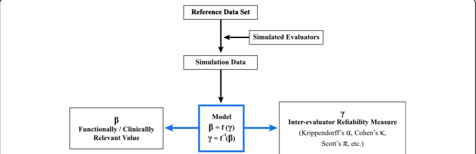
clinically-relevant value. Our approach involves generat-ing a large population of simulated evaluator data, and then calculating the error and agreement of each against a reference dataset. This creates a model between evalu-ator agreement and error, that describes how much error could be expected based on any given level of agreement
(Fig. 1). The below step-by-step approach describes how
this method is generally applied. The instructions are intended for investigators with a modest background in mathematics, statistics, and basic programming (such as
MATLAB). The simulation time will vary based on sev-eral factors (calculation optimization, dataset size, simu-lation iterations, etc.). For our quantitative example, the simulation and calculations took approximately 1 to 2 h to run on a standard office desktop computer.
Establish a reference dataset
A reference dataset must be established for the evalu-ator test that is being modelled. The only requirement for the reference dataset is that it is representative of a typical dataset from that test. The reference dataset is
not required to be empirical data; rather, the reference
dataset could be generated from a distribution of, or a
distribution parameterized to resemble, a population of test scores. This reference dataset will be used as a basis for generating and comparing the simulated evaluator population. There are no specific require-ments for the length of the reference dataset. The au-thors do not wish to conjecture on the appropriate amount of data to be used when working with reliabil-ity indices, as the answer is likely context-sensitive, and
has been investigated by others [25,26]. At a minimum,
it would seem necessary to include at least the same amount of data that would be used in a practical appli-cation or research study using that reliability index. For example, if one were generating a model to provide context to field applications of inter-evaluator reliability measures, then using a reference dataset of the same size that has been determined appropriate for those field applications would likely provide the most relevant model. It should be noted that the reference dataset is
not required to be single instance of an evaluator test, but instead could be a concatenation of results from multiple independent instances of that test.
Mathemat-ically, we will refer to the reference dataset asIm, where
mis the number of measurements in the dataset.
Simulate a population of evaluators
For purposes of simplification, the reference dataset can
now be thought of as a “perfect evaluator.” That is, the
reference dataset is considered to be the result of an evaluator who is perfectly reliable, and has obtained the
“correct” answer from evaluating the test. As stated
above, the reference data do not need to be correct (or even empirical data), they are only referred to as correct for purposes of generating the model because they are used as a basis of comparison. Their actual correctness
has no bearing on the model’s accuracy or validity. Each
new evaluator is simulated by taking the reference data-set and introducing Gaussian noise into it. Taylor has shown that a Gaussian distribution is a valid first-order approximation of the two observational errors that are inherent to any system of measurement: systematic
er-rors and random erer-rors [27]. These errors can be
mod-elled by modifying the first (mean) and second (standard deviation) moments of the Gaussian distribution,
re-spectively [27]. In essence, the Gaussian distribution can
be thought of as an evaluator whose likelihood of mak-ing a systematic error or random error is described by the mean and standard deviation of the Gaussian distri-bution. For example, an evaluator who makes systematic errors is described by a Gaussian distribution with a shifted mean (errors are systematically in the same dir-ection) whereas an evaluator who makes random errors is described by a Gaussian distribution with a large standard deviation (errors randomly fall on either side of the average measurement). In practice, evaluator mis-takes may not be perfectly Gaussian, but over many sim-ulated trials, all evaluator errors would tend to a Gaussian distribution due to the central limit theorem.
A set of random variables from Gaussian distributions
(we will call this set “X”) must be generated to capture
at least the range of evaluator behavior that may be practically expected; additional distributions may be gen-erated to capture more erroneous behavior, but this may incur additional computation time. The total number of
random Gaussian variables (the size of set X) generated
will depend on the chosen step-size and range of sys-tematic error and random error to be investigated, and this is heavily dependent on the specific task. In many cases, it may be appropriate to increment systematic error and random error by the resolution of rating units used in the test (i.e., the smallest change in measure-ment an evaluator can make). If a continuous scale is be-ing used, an appropriate error step-size will have to be determined; there is no set procedure for determining the error step-size, and this will have to be done at the discretion of the investigator. A general rule might be to use the smallest step-size that is still detectable or has meaningful relevance to the test (e.g., a step-size of one nanosecond would be too fine of a resolution for a
human reaction time task, whereas a step-size of a sec-ond would be too coarse). In the case of nominal data, where only two rating units are available, the error step-size may be thought of as a probability step-size. It should be noted that this method allows for the step-size and range of systematic error and random error to be chosen independently.
The chosen values of systematic error to investigate
will be represented by the arrayμ, and the length of that
array (the chosen range of error divided by the chosen
resolution) will be referred to as, and indexed by,i.
Simi-larly, the values of random error will be represented by
the array σ, and the length of that array will be referred
to as, and indexed by, j. Additionally, theμ andσarrays
should each contain the value“0,”representing an
evalu-ator who does not make that type of measurement error. Therefore, the equation
Xij N μi;σj
ð1Þ
describes aniby jmatrix of Gaussian random variables, whereiandjindex the mean (μ) and standard deviation (σ) of theXijGaussian distributions from which the
ran-dom variables were generated, respectively. New i * j Gaussian random variables are generated along them di-mension, so that there are i by j random variables for eachmmeasurement in the reference dataset. Next, the reference dataset,Im, must be replicated along theiand jdimensions. Thus,Iijmis a matrix of the reference data and there are i * j copies of each m measurement, so that each m measurement can be modified by each ij Gaussian random variable. The final step is to generate the simulated evaluator population,I′, calculated as
I0ijm¼Iijmþ Xijm: ð2Þ
Each element of Iijm is modified by a random value
generated from one of the Gaussian distributions, whose
parameters are described by i and j. The result is a
population of simulated evaluators, matrix I’ijm. Each ij
evaluator, whose measurement errors are described by
Xij, has made m measurements. As previously stated,
the evaluator whose μ= 0 andσ= 0 is the perfect
evalu-ator (the initial reference dataset) who will be the basis of comparison for all other simulated evaluators.
This process relies on the sampling of random
vari-ables (Xijm), and therefore the simulation should be
re-peated N multiple times. This smooths the randomness
of the data and allows for a more robust model. Our methodology has no inherent requirements about the number of times the simulation should be repeated. Many others have investigated optimal sample sizes for
simulation studies [28, 29], and their work may be
simulations improves the final result but increases com-putation time. Thus, the result of the simulation should
be i * j evaluator datasets of length m, where each ijm
combination has been simulated N times (with each
simulation samplingijmnew random variables from the
ijGaussian distributions).
Create the model
Once the evaluator population has been simulated,
agree-ment and error must be calculated for each of theN * i * j
evaluators. In other words, each combination of i and j
must be compared to the μ= 0, σ= 0 perfect evaluator
(the reference dataset). Our method is not limited to any particular agreement or error calculation, so this step is dependent on the reliability index and error calculation that are most appropriate to the evaluator task. However, the manner in which agreement and error measures are calculated should be reflective of how they would be ap-plied in practice. For example, if the result of an evaluator
test is interpreted byaddingall of the evaluator’s
individ-ual scores together, then error should be calculated on this
sum. Alternatively, if an evaluator’s results are interpreted
by averaging all of their individual scores together, then
error should be calculated on thisaveragedscore.
Gener-ally, it is likely that the best method for calculating agree-ment is to compare each individual score between the evaluators. However, it is most important that agreement is calculated in the way that has been deemed most appro-priate for the practical application or research study, as this will provide the most relevant model between agree-ment and error.
Once agreement and error have been calculated for each evaluator relative to the reference dataset, agree-ment and error should be averaged by observational
error parameters across all Nsimulations. That is, every
evaluator who had both the sameμand σcould be
con-sidered to have been the same evaluator (as they were exactly as probable to make the same mistakes), and
therefore their agreement and error from all N
simula-tions should be averaged together to quantify their aver-age performance, thus smoothing the simulated data.
This should result in i * j four-dimensional datasets
which each contain an agreement, error,μi, andσjvalue,
one for eachi * jevaluator. The agreement and error of
all evaluators can now be plotted against each other to model how much error can be expected from an evalu-ator based on their level of agreement. Optionally,
sys-tematic error (μi) and random error (σj) can be plotted
for each evaluator (e.g., by color or size of markers, see below for example) to further understand how observa-tional errors affect agreement and error. It would
gener-ally be expected that an envelope would form;
essentially, this is a boundary that emerges which de-scribes the most amount of error (worst-case error) an
evaluator could be expected to have, based on their cal-culated agreement. We demonstrate this below in our quantitative example. A function may be fit to this enve-lope which allows a mathematical description relating agreement and worst-case error.
Quantitative example
This quantitative example is provided to illustrate how the method is applied, and because it was a practical challenge that we encountered in our research; the solu-tion to which was the basis of this general method. Again, it is important to clarify that the specifics of how the method is applied (agreement measure, error meas-ure, etc.) to this evaluator task are not due to inherent limitations of the method, rather, our selected reliability index, error measure, error-step size, etc., were chosen as the most appropriate for our particular evaluator task.
Establish a reference dataset
Three research professionals analyzed video footage, with the goal of improving internal processes. They judged and recorded times of two distinct reoccurring events. The video was obtained under a Defense Ad-vanced Research Projects Administration research study and contained footage of an anonymous consented par-ticipant transferring rubber blocks between two com-partments of a wooden box. Evaluators worked in isolation using media player software which allowed for-ward and backfor-ward frame-by-frame scrubbing. They scanned through the video and determined the times at which the participant grasped blocks in one compart-ment and the times at which they released them into the other compartment. They recorded these video timing events into a spreadsheet, producing a total of 300 tim-ing measurements for each evaluator. Each individual timing event was taken and averaged across the three expert evaluators to produce a single representative 300-point reference dataset.
Simulate a population of evaluators
We wrote a custom MATLAB (Mathworks, Natick, MA) script to create 49 unique simulated evaluators by inject-ing error into the reference dataset. To do this, the script generated 49 Gaussian distributions, each with different combinations of mean and standard deviation parameters,
which represented systematic error (μ) and random error
(σ), respectively. In other words, each of the 49
combina-tions ofμandσgenerated a distinct Gaussian distribution,
where each Gaussian distribution represented the obser-vational errors made by different simulated evaluators. The analyzed video footage was recorded at 30 frames per
second, so the step-size forμandσof the Gaussian
distri-butions was chosen to be 0.033 s (one video frame), the
0 to 0.198 s (0 to 6 video frames), for a total of 49
combi-nations. In cases whereμ was low andσwas high, some
simulated evaluators occasionally selected negative values (about 0.3% of measurements). While our chosen range of random error resulted in this unrealistic circumstance, we wanted to ensure that we captured a sufficient range of evaluator error to build our model. In our application, negative and zero-duration timing events were not pos-sible, so these values were defaulted to 0.033 s (the mini-mum resolvable time for an event, one video frame). This introduced a small amount of bias to cases with high ran-dom error relative to systematic error which can be seen in the results; we discuss this in more detail below.
Three hundred random numbers were then chosen from each of the 49 Gaussian distributions and added to the refer-ence dataset to create 49 new unique hypothetical datasets each containing 300 modified timing values, as described
above in Eqs. (1) and (2). In other words, each simulated
evaluator made 300 different“mistakes”, one for each of the
300 measurements, with each error drawn from the
evalua-tor’s own Gaussian distribution. Each of the 49 modified
datasets represented a set of 300 imperfect scores generated by a simulated evaluator. It should be noted that our choice of using 300 measurements reflects how we would use inter-evaluator agreement in a practical application. That is, a complete execution of the test produces 300 measure-ments, and we would ideally measure inter-evaluator agree-ment on a full test dataset; thus, we chose to generate our model using a full 300-measurement dataset.
To smooth the randomness of the data, we repeated this process 100 times for each of the 49 Gaussian distribu-tions. We stopped the simulation after 100 iterations, as this produced a smooth monotonic relationship between increasing random error and decreasing inter-evaluator agreement, which we deemed appropriate for our specific application. This resulted in 4900 unique hypothetical datasets. These new hypothetical datasets were then used
as the “results” obtained from 49 simulated evaluators,
each completing the video analysis task 100 times.
Create the model
The Krippendorff’s alpha and percent error were then
calculated for each of the 4900 datasets, pairwise with the reference dataset, to explore relationships between
Krippendorff’s alpha, percent error, systematic error,
and random error. We specifically chose Krippendorff’s
alpha as it was appropriate in the application of our data, which were time measurements (ratio data type).
Krippendorff explains in detail how Krippendorff’s
alpha is calculated in his 2011 manuscript [30]. Here,
we briefly summarize the calculation. We wrote a cus-tom LabVIEW (National Instruments, Austin, TX) pro-gram which used the coincidence matrix calculation
method (Eq.3),
α¼1−ðn−1Þ
P c
P
k ock δ
metric
2
ck P
c X
k ncnk metricδ2ck;
ð3Þ
and verified the accuracy of our program with ReCal OIR
[30,31]. Equation3was used for all Krippendorff’s alpha
calculations, wherenis the total number of measurements
collected,candkare each a separate index into the same
set of unique values that increment independently to allow for generation of every allowable pairwise combination.
The allowable pairwise combinations arexcandxk(the
re-liability data, see Eq.4) for all possible values of cand k
whereasncandnkare the number of times thatxcandxk
are used in total. The number of occurrences ofxcandxk
value pairings within the reliability data are represented by
ock. The type of reliability data being used dictates which
“difference function” to use, defined as δmetric2ck, where
metric is the data type. The difference function for ratio
data is shown in Eq. (4):
δ
ratio 2ck¼ xc−xk xcþxk
2
: ð4Þ
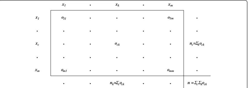
We used the coincidence matrix to calculate
Krippen-dorff’s alpha because it is the most computationally
effi-cient method (Fig.2). For our percent error calculations
(Eq. 5, whereTheoretical is the reference measurement
andExperimentalis the simulated measurement),
Percent error¼jTheoretical−Experimentalj
Theoretical 100; ð5Þ
we decided what part of the task provided the highest
level of error. In our video rating task, the“speed”phase
squared error, or some other calculation to quantify the error of an evaluator. We constructed the model for this
task using the Krippendorff’s alpha and percent error
calculations.
Model assessment
We wanted to verify that our model accurately described the relationship between the agreement and error of ac-tual human evaluators, and also demonstrate the applic-ability of the model in a real-world scenario. We first fit
a curve (y =−0.637x1.76+ 1, r2= 0.999; the curve was
created using Igor Pro v 6.36 Curve Fitting function; WaveMetrics, Portland, OR) to the model, using the data points of simulated evaluators who defined the en-velope, to mathematically define what would be the
“worst-case” percent error for any given Krippendorff’s
alpha value (see Results). A power law was chosen for
the curve fit as it provided a high r2 for the envelope,
over the range of data that we were interested in. This is, again, a facet of the methodology that is dependent on the evaluator task; our methods are generalizable to allow any form of curve fitting. We then compared the results of the hypothetical modeling to an actual popula-tion of evaluators to demonstrate that the model values reflect the values actually generated by human evalua-tors. To do this, we assigned the video analysis task to a
new cohort of trained human evaluators (n= 5). We
used the reference dataset from our panel of expert eval-uators (described above) as a standard of comparison
and calculated Krippendorff’s alpha and percent error
values for each of the human evaluators to verify their compliance to the model.
Since the test data that were used to generate the model were also the same data that the evaluators were scoring, it was a concern that any comparisons between the evalu-ators and the model were circular and not generalizable to
new instances of the test. To explore this idea we repeated all of the simulation steps using a new scoring video of a different anonymous participant taking the same test, scored by a new evaluator. All error step-sizes, error cal-culations, and agreement calculations were methodologic-ally identical to the original simulation described in
“Quantitative example”. We again plotted the results of
the human evaluators from theoriginalvideo analysis, to
see if they were still well-explained by the new model, as
well as fit a curve to the new envelope (y =−0.6251x1.685
+ 1.001, r2= 0.9998) to determine if there was any change
between the two models in the mathematical relationship between agreement and error.
Results
The Krippendorff’s alpha values for the 4900
hypothet-ical datasets ranged from 0.998 to 0.854 and the percent
error values ranged from 0 to 39.4%. Figure3shows the
average Krippendorff’s alpha and average percent error
of all 49 (averaged) simulated evaluators, with the size and shading of the markers representing the random error and systematic error parameters, respectively. For our evaluator task an increase in systematic error was
correlated to an increase in percent error (Pearson’sr=
0.997, p< 0.001), whereas random zero-mean error did
not correlate to an increase percent error (Pearson’sr=
−0.025, p= 0.865). This was a result of our task being
specifically concerned with average percent error; simu-lated evaluators with zero-mean random error produced modest percent error when averaged over many trials.
As seen in Fig. 3, this result was also evidenced by
dar-ker circles falling farther to the right with larger circles of the same color aligning vertically. As mentioned above, flooring our measurements to 0.033 s introduced a small amount of systematic error into simulated evalu-ators who were prescribed low systematic error and high
random error. This can be seen in Fig. 3as the markers with increasing random error are staggered to the right when systematic error is low. This deviance was not a concern for our specific investigation as we were only interested in the envelope of the model.
Model assessment
To verify that our model accurately described the evalu-ator agreement and measurement error relationship of
actual human evaluators, we plotted the Krippendorff’s
alpha and percent error values collected from our hu-man evaluators against the perforhu-mance of the simulated evaluators. We found that the results of the human
evaluators fell within the envelope defined by the
simu-lated evaluator performance (Fig.4).
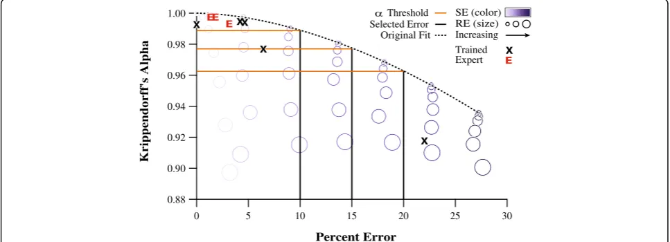
Figure5 shows the model created using the results of
the new trained evaluator analyzing this new instance of the block moving task. The original fit from the model
in Fig. 4 still provides an accurate description of the
Krippendorff’s alpha and percent error relationship (r2=
0.991). The lighter dotted line is the new fit (y =−
0.6251x1.685+ 1.001, r2= 0.9998) and is provided for
comparison. The two models are highly similar, and are nearly identical when considering percent error of 10% or less. Both models show high agreement and low error for the tightly clustered six evaluators, who would pass
1.00
0.98
0.96
0.94
0.92
0.90
0.88
Krippendorff's Alpha
30 25
20 15
10 5
0
Percent Error
RE (size) Increasing SE (color)
Fig. 3This scatterplot shows the average Krippendorff’s alpha and percent error values for each of the 49 simulated evaluators, with the size and shading of the markers representing random error and systematic error, respectively. An envelope exists which describes the upper-bound of percent error for any given value of Krippendorff’s alpha for this video analysis task
1.00
0.98
0.96
0.94
0.92
0.90
0.88
Krippendorff's Alpha
30 25
20 15
10 5
0
Percent Error Threshold Selected Error Original Fit
Expert Trained RE (size) Increasing SE (color)
any of the example Krippendorff’s alpha thresholds pre-sented, and one evaluator who has relatively low agree-ment and excessively high error that would not pass any of the thresholds.
Discussion
When measuring agreement between evaluators, a de-cision about what constitutes an acceptable level of agreement must be made. Historically, interpreting an agreement measure was ambiguous, as the practical implications of choosing one threshold over another were not well-defined. This led to general use of a
0.8 “rule of thumb” value as a threshold, though
sev-eral works have suggested that this cut-off is not
likely suitable for all studies [4, 10, 13–16]. To
ad-dress this issue, we developed a systematic approach to arrive at a relevant context-specific reliability threshold, bridging the gap between reliability indices and the error inherent to the test construct of inter-est. Our approach simulated the results of a large population of evaluators. In our quantitative example,
these simulated evaluators “judged” a video analysis
task. Our method injected known tendencies for mak-ing systematic and random errors, and calculated the
agreement (Krippendorff’s alpha in our example) and
the error (percent error in our example) between the simulated data and a reference dataset. This proced-ure allowed us to relate agreement, which is custom-arily measured in reliability studies, to the amount of
error from the “true” values, which is more salient
but typically unavailable. In our example, we found that an envelope existed which defined the maximum observed percent error for any given value of
Krip-pendorff’s alpha. We characterized this envelope and
determined its effectiveness and generalizability.
During the evaluation of our quantitative example, we found that the results of the human evaluators adhered to the derived threshold envelope and were similar to those
obtained from the simulated data (Fig. 4). As evidenced
through this quantitative example, these findings support that our proposed techniques have the power to facilitate meaningful interpretations of reliability indices in a rele-vant context of measurement error. An additional
charac-teristic of our quantitative example is highlighted in Fig.6.
Here, the contour plots, generated using the simulated
datasets, show Krippendorff’s alpha (left) and percent
error (right) values for the investigated combinations of systematic error and random error. It was demonstrated that an increase in either systematic error or random error
can lead to a decrease in agreement (lower Krippendorff’s
alpha), whereas percent error (the “functional value”), on
average, is only affected by systematic error. This is due to the mathematical nature of random observational errors (and thus how they were modeled), as they are described by symmetrical deviations with no net change from the mean of a Gaussian distribution; therefore, they average to
zero over many trials [27]. This contour plot format can
be more generally applied to other reliability indices or measures of errors to illustrate the consequences of obser-vational errors.
Finally, the data highlighted in Fig. 5 were generated
from a new participant being scored by a new evaluator to verify the generalizability of our techniques. The only observed difference between this newly generated model and the original was that the contour plots (not shown)
of Krippendorff’s alpha and percent error were
com-pressed, as the values from the second test were, on average, numerically smaller than the first test. This means that systematic error and random error had
rela-tively greater effects on Krippendorff’s alpha and percent
1.00
0.95
0.90
0.85
0.80
Krippendorff's Alpha
40 30
20 10
0
Percent Error
RE (size) Increasing SE (color) Threshold
Selected Error Original Fit
Expert New Fit
Trained
error. Regardless, the Krippendorff’s alpha and percent error relationship generated by this model remained a valid and useful way to assess evaluator reliability in this video analysis task. This was evidenced by re-plotting the human evaluators on the new model, as they fell within similar error and agreement thresholds as the
ori-ginal model (Fig.5). These data suggest that once a
rela-tionship between a selected reliability index and functional measure has been established, that result is generally applicable to any instance of that same test, scored by any cohort of evaluators, without need to re-visit the model.
This example demonstrates the use of our systematic procedure to both investigate the consequences of differ-ent agreemdiffer-ent thresholds and provide a framework for researchers to make informed decisions about reliability in their evaluator-based tests. Modeling a large popula-tion of evaluators with a variety of prescribed probabil-ities for making mistakes and then calculating their resulting error allowed us to describe our chosen agree-ment measure in the context of how the data would be used practically. In our example, we generated a stand-ard of comparison for this specific instance of our test by employing a group of expert evaluators. Comparing
the experts’results to the trained evaluators’results
re-vealed practicable levels of agreement and the error as-sociated with that agreement. We found that high levels of agreement (0.99 and up) were regularly achieved and
afforded error of no greater than 5%. Using our model as a frame of reference we concluded that a
Krippen-dorff’s alpha threshold of 0.985 should be used for this
task to permit error no greater than 12% while not being so strict as to potentially throw out useful data. It is crit-ical to note that the conventional 0.8 rule of thumb threshold would have been egregiously permissive in our quantitative example, further reinforcing the need for application-specific agreement thresholds.
A key strength of our methodology is its high level of customizability which greatly expands its scope and util-ity. This procedure should be applicable to most any agreement measure or evaluator-based task, and may be uniquely tailored to emphasize the important aspects of the task or to reflect how the data will be used in prac-tice. The investigator may choose the step-size of the
simulated evaluators’errors and the approach for
calcu-lating error (using percent error or a different error cal-culation entirely, calculating error on individual values or averages values, etc.) beforehand, based on the spe-cific needs of that test. Additionally, the investigator is
able to decide how the “true” or reference data that are
used for calculating agreement and error are defined or generated. It should be noted that the presence of true or even presumably-true values are not necessary for using this method, and the values used to generate the model are not even required to be actual results from the specific test of interest. The only requirement for 0.977
0.977
0.993 0.9930.9950.995
0.998 0.998 0.998 0.998 0.918 0.918 0.198 0.165 0.132 0.099 0.066 0.033 0.000
Random Error (
seconds) 0.977 0.9930.995 0.993 0.998 0.994 0.998 0.99 0.98 0.97 0.97 0.96 0.95 0.94 0.93 0.92 0.92 0.92 0.91 0.918 0.198 0.165 0.132 0.099 0.066 0.033 0.000
Systematic Error ( seconds) 0.198 0.165 0.132 0.099 0.066 0.033 0.000 0.198 0.165 0.132 0.099 0.066 0.033 0.000 6.48 6.48 3.12 3.124.204.20
0.03 0.03
1.79 1.79 1.33 1.33 4.644.64
22.03 22.03 6.48 3.124.20 0.03 1.79 1.33 26 26 24 24 24 22 20 18 18 16 16 14 14 12 12 12 10 10 8 8 6 6 4 4 2 2 10 6 8 4.64 22.03
these reference data is that they are representative of the types of values resulting from an evaluator judging the specific test. In our quantitative example, the error step-size was chosen to be the resolution of the mea-surements of the test (based on the video frame rate). We used percent error calculations from a subset of the measurements which represented a particular metric of interest. We determined this metric to be most sensitive to error so using it for our calculations provided us with a worst-case percent error for any given level of
agree-ment. The“true”or reference values were established by
averaging together the results of the expert evaluators. Our methodology may provide a useful framework for establishing agreement benchmarks in evaluator-based tests, and could be adapted for application in other con-texts. For example, the reliability of clinical tests which require human evaluation is a major concern. The accur-acy and validity of these types of assessments could be improved by using our methodology. To implement our methods more generally into a clinical context (or other evaluator-based applications), a possible approach would
be first building a “true” or reference set of
measure-ments for a typical application of the test. A baseline panel of expert evaluators could be employed to gener-ate the reference measurement(s) for that particular ap-plication. Modeling a simulated evaluator population from this dataset would establish an agreement-error
re-lationship that could be used as a“grading scale,” to
re-late evaluator quality (inter-evaluator reliability) and measurement error, that would generally apply in any in-stance of that test. This process would only need to be performed once, and the resulting scale could then be incorporated into training programs for new evaluators or used to periodically assess groups of existing evalua-tors as a measure of quality control.
Perhaps the biggest limitation of this work is that the models generated are inherently more accurate when the reference data are of similar numerical magnitude to the data typically obtained from the testing procedure.
Al-though a“one size fits all” solution would be ideal,
mul-tiple models may be necessary if the results of the evaluator task vary greatly. For instance, in our quantita-tive example, video footage of a healthy participant trans-ferring objects with their upper limbs was scored. If this task were performed with a sensorimotor-impaired par-ticipant, where scores would be anticipated to differ sig-nificantly from healthy performance, it may be necessary to generate a new model built from reference data that are more reflective of the anticipated sensorimotor-impaired results. Further work could be done to investigate the consistency of models over different ranges of numerical values and how, and to what extent, the models diverge from the data. This methodology could potentially reveal strengths and weaknesses of different reliability indices
and possibly inform the selection of an appropriate agree-ment measure. Our approach of using zero-mean random error may present as a limitation as it is an idealized cir-cumstance. This zero-mean approach could perhaps be replaced with a more nuanced approach exploring the skew and kurtosis of error distributions to potentially re-veal additional findings. Skew and kurtosis may have the potential to model more peculiar erroneous evaluator be-havior, such as heavy-tailed outlier data, which could be approximated by increased kurtosis. A particularly troublesome example would be an evaluator who occa-sionally selects extreme values in an asymmetric fashion to intentionally bias the outcome of an evaluation. Our methodology could be used to model what this behavior looks like from a reliability perspective, to help detect and mitigate this type of behavior in the field.
This work aims to provide a generalizable procedure, yet datasets in evaluator-based scoring activities may be diverse in size, variability, and data type. Thus, it is not feasible to devise a universal procedure which can ac-commodate all possible variants of reliability data. As such, each individual application of this methodology requires the discretion of the investigator. Furthermore, this method could reasonably apply to many data types (e.g., nominal, interval, ratio), error measurements (e.g., percent error, RMS error, mean absolute error), and
re-liability indices (e.g., Cohen’sκ, Scott’sπ, Krippendorff’s
α). We suggest that the quantitative basis of this
method represents an improvement over rule of thumb conventions for interpreting reliability indices.
Conclusion
By simulating a population of evaluators with predeter-mined probabilities for making mistakes, we have explored correlations between evaluator reliability indices and func-tional test values of interest. We demonstrate this method using a quantitative example to derive a relationship
be-tween Krippendorff’s alpha and percent error. Through
this simulation and modeling we assessed the quality of our human evaluators based on their alpha coefficients. We propose that this is a reasonable technique for estab-lishing agreement thresholds to identify suitable evalua-tors and this technique could be expanded for use in other evaluator-based tests, or with different agreement and/or error measurements.
Acknowledgments
We thank Jon Sensinger for input on the manuscript.
Funding
Availability of data and materials
All relevant data are contained within the paper and are freely available without restriction.
Authors’contributions
DTB contributed to data collection and analysis. ZCT and PDM contributed to analyses. All authors contributed to writing the manuscript. All authors read and approved the final manuscript.
Ethics approval and consent to participate
This modeling project was undertaken to improve internal processes for establishing reliability of evaluators and deemed not subject to IRB review. The block transfer metrics and video footage of fully consented study participants were covered by Cleveland Clinic IRB approved study 13–1349 Sensory Feedback Tactor Systems for Implementation of Physiologically Relevant Cutaneous Touch and Proprioception with Prosthetic Limbs.
Consent for publication
Informed consent for the Cleveland Clinic IRB approved study 13–1349 Sensory Feedback Tactor Systems for Implementation of Physiologically Relevant Cutaneous Touch and Proprioception with Prosthetic Limbsincludes consent for publication.
Competing interests
The authors declare that they have no competing interests.
Publisher’s Note
Springer Nature remains neutral with regard to jurisdictional claims in published maps and institutional affiliations.
Received: 8 June 2018 Accepted: 2 November 2018
References
1. Feng GC. Factors affecting intercoder reliability: a Monte Carlo experiment. Qual Quant. 2013;47:2959–82.
2. Antoine J-Y, Villaneau J, Lefeuvre A. Weighted Krippendorff’s alpha is a more reliable metrics for multi-coders ordinal annotations: experimental studies on emotion, opinion and coreference annotation. In: Proc 14th Conf Eur Chapter Assoc Comput Linguist; 2014. p. 550–9.http://www. aclweb.org/anthology/E14-1058.
3. Krippendorff K. Content analysis: an introduction to its methodology. Beverly Hills: Sage Publications; 1980.
4. Craggs R, Wood MM. Evaluating discourse and dialogue coding schemes. Comput Linguist. 2005;31:289–96.
5. Hayes AF, Krippendorff K. Answering the call for a standard reliability measure for coding data. Commun Methods Meas. 2007;1:77–89. https://doi.org/10.1080/19312450709336664.
6. Oleinik A, Popova I, Kirdina S, Shatalova T. On the choice of measures of reliability and validity in the content-analysis of texts. Qual Quant. 2014;48: 2703–18.
7. Krippendorff K. Agreement and information in the reliability of coding. Commun Methods Meas. 2011;5:93–112.
8. Bartlett JW, Frost C. Reliability, repeatability and reproducibility: analysis of measurement errors in continuous variables. Ultrasound Obstet Gynecol. 2008;31:466–75.
9. Lombard M, Snyder-Duch J, Bracken CC. Content analysis in mass communication: assessment and reporting of Intercoder reliability. Hum Commun Res. 2002;28:587–604.
10. Krippendorff K. Reliability in content analysis: some common
misconceptions and recommendations. Hum Commun Res. 2004;30:411–33. 11. Banerjee M, Capozzoli M, McSweeney L, Sinha D. Beyond kappa: a
review of interrater agreement measures. Can J Stat. 1999;27:3–23. https://doi.org/10.2307/3315487.
12. Zwick R. Another look at interrater agreement. Psychol Bull. 1988;103:374–8. 13. Artstein R, Poesio M. Inter-coder agreement for computational linguistics.
Comput Linguist. 2008;34:555–96.https://doi.org/10.1162/coli.07-034-R2. 14. Carletta J, Carletta J, Computational I, Computational I. Squibs and
discussions assessing agreement on classification tasks: the kappa statistic. Comput Linguist. 1993;22:248–54.
15. Eugenio BD, Glass M. The kappa statistic: a second look. Comput Linguist. 2004;30:95–101.https://doi.org/10.1162/089120104773633402. 16. Reidsma D, Carletta J. Reliability measurement without limits. Comput
Linguist. 2008;34:319–26.https://doi.org/10.1162/coli.2008.34.3.319. 17. Wilhelm AG, Rouse AG, Jones F. Exploring differences in measurement and
reporting of classroom observation inter-rater reliability. Pract Assess Res Eval. 2018;23:1–16.
18. Stilma W, Rijkenberg S, Feijen H, Maaskant JM, Endeman H. Validation of the Dutch version of the critical-care pain observation tool. Br Assoc Crit Care Nurses. 2015; Epub ahead of print.
19. van Veen MJ, Birnie E, Poeran J, Torij HW, Steegers EAP, Bonsel GJ. Feasibility and reliability of a newly developed antenatal risk score card in routine care. Midwifery. 2015;31:147–54.https://doi.org/10.1016/j.midw.2014.08.002. 20. Rohan KJ, Rough JN, Evans M, Ho SY, Meyerhoff J, Roberts LM, et al. A protocol
for the Hamilton Rating Scale for Depression: item scoring rules, rater training, and outcome accuracy with data on its application in a clinical trial. J Affect Disord. 2016;200:111–8.https://doi.org/10.1016/j.jad.2016.01.051. 21. Swanton AR, Arlen AM, Alexander SE, Kieran K, Storm DW, Cooper CS.
Inter-rater reliability of distal ureteral diameter ratio compared to grade of VUR. J Pediatr Urol. 2017;13:207.e1–207.e5.https://doi.org/10.1016/j.jpurol.2016.10.021. 22. Wikstrom EA, Allen G. Reliability of two-point discrimination thresholds
using a 4-2-1 stepping algorithm. Somatosens Mot Res. 2016;33:156–60. 23. De Groef A, Van Kampen M, Vervloesem N, Clabau E, Christiaens MR, Neven P,
et al. Inter-rater reliability of shoulder measurements in middle-aged women. Physiother apy. 2017;103:222–30.https://doi.org/10.1016/j.physio.2016.07.002. 24. Kvistgaard Olsen J, Fener DK, Wæhrens EE, Wulf Christensen A, Jespersen A,
Danneskiold-Samsøe B, et al. Reliability of pain measurements using computerized cuff algometry: a DoloCuff Reliability and Agreement Study. Pain Pract. 2017;17:708–17.
25. Saito Y, Sozu T, Hamada C, Yoshimura I. Effective number of subjects and number of raters for inter-rater reliability studies. Stat Med. 2006;25:1547–60. 26. Walter SD, Eliasziw M, Donner A. Sample size and optimal designs for
reliability studies. Stat Med. 1998;17:101–10.
27. Taylor JR. An introduction to error analysis the study of uncertainties in physical measurments. 2nd ed. Sausalito: University Science Books; 1997. 28. Hahn GJ. Sample sizes for Monte Carlo simulation. IEEE Trans Syst Man
Cybern. 1972;2:678–80.
29. Cassettari L, Mosca R, Revetria R. Monte Carlo simulation models evolving in replicated runs: a methodology to choose the optimal experimental sample size. Math Probl Eng. 2012;2012:1–17.
30. Krippendorff K. Computing Krippendorff’s alpha-reliability. Dep Pap. 2011;1–12.https://repository.upenn.edu/cgi/viewcontent.cgi?article= 1043&context=asc_papers.