RESEARCH
Implications of allometric model
selection for county-level biomass mapping
Laura Duncanson
1,2*, Wenli Huang
2, Kristofer Johnson
3, Anu Swatantran
2, Ronald E. McRoberts
4and Ralph Dubayah
2Abstract
Background: Carbon accounting in forests remains a large area of uncertainty in the global carbon cycle. Forest aboveground biomass is therefore an attribute of great interest for the forest management community, but the accuracy of aboveground biomass maps depends on the accuracy of the underlying field estimates used to calibrate models. These field estimates depend on the application of allometric models, which often have unknown and unre-ported uncertainties outside of the size class or environment in which they were developed.
Results: Here, we test three popular allometric approaches to field biomass estimation, and explore the implica-tions of allometric model selection for county-level biomass mapping in Sonoma County, California. We test three allometric models: Jenkins et al. (For Sci 49(1): 12–35, 2003), Chojnacky et al. (Forestry 87(1): 129–151, 2014) and the US Forest Service’s Component Ratio Method (CRM). We found that Jenkins and Chojnacky models perform comparably, but that at both a field plot level and a total county level there was a ~ 20% difference between these estimates and the CRM estimates. Further, we show that discrepancies are greater in high biomass areas with high canopy covers and relatively moderate heights (25–45 m). The CRM models, although on average ~ 20% lower than Jenkins and Chojnacky, produce higher estimates in the tallest forests samples (> 60 m), while Jenkins generally produces higher estimates of biomass in forests < 50 m tall. Discrepancies do not continually increase with increasing forest height, suggesting that inclusion of height in allometric models is not primarily driving discrepancies. Models developed using all three allometric models underestimate high biomass and overestimate low biomass, as expected with random forest biomass modeling. However, these deviations were generally larger using the Jenkins and Chojnacky allometries, suggesting that the CRM approach may be more appropriate for biomass mapping with lidar.
Conclusions: These results confirm that allometric model selection considerably impacts biomass maps and estimates, and that allometric model errors remain poorly understood. Our findings that allometric model discrep-ancies are not explained by lidar heights suggests that allometric model form does not drive these discrepdiscrep-ancies. A better understanding of the sources of allometric model errors, particularly in high biomass systems, is essential for improved forest biomass mapping.
Keywords: Forest biomass, Lidar, Allometry, Carbon accounting
© The Author(s) 2017. This article is distributed under the terms of the Creative Commons Attribution 4.0 International License (http://creativecommons.org/licenses/by/4.0/), which permits unrestricted use, distribution, and reproduction in any medium, provided you give appropriate credit to the original author(s) and the source, provide a link to the Creative Commons license, and indicate if changes were made.
Background
Forest aboveground biomass mapping has emerged as a critically important initiative for both constrain-ing the global carbon cycle [18] and facilitating climate mitigation initiatives such as REDD+ [8]. Estimates of
aboveground biomass are typically generated through a combination of field sampling and extrapolation using remote sensing data [9]. Lidar remote sensing, in par-ticular, has emerged as a popular technology for map-ping aboveground biomass in high biomass systems, as there is no apparent saturation of lidar metrics with high biomass provided that the lidar pulses penetrate to the ground [22]. However, the accuracies of all remote sensing-based biomass maps are inherently dependent
Open Access
*Correspondence: [email protected]
2 Department of Geographical Sciences, University of Maryland, College
Park, USA
on underlying accuracies of the field estimates of biomass that are used to calibrate remote sensing-based models.
Field estimates of biomass are generally estimated through the application of an allometric model relat-ing some measurable attribute of field biomass, e.g. tree stem diameter or height, to aboveground biomass [5, 12]. These allometric models are typically developed through the destructive sampling of a relatively small number of trees, which are directly measured for their biomass. As destructive samples are costly to acquire, the sample sizes used to construct allometric models tend to be relatively small and spatially clustered [7]. As such, the accuracies of these allometric models outside their areas of develop-ment remain largely unknown due to a dearth of avail-able sampled validation data [3]. Therefore, determining which allometric model to select for the estimation of field biomass is largely speculative.
In the United States, the two most common sets of allometric models are (a) a set of generalized models developed through a meta-analysis of the literature [12], and (b) the US Forest Service’s Component Ratio Method (CRM) [10, 20]. Jenkins et al. [12] combined thousands of allometric models that performed destructive sampling of trees, and simplified them to just 10 models for gen-eral applicability. The Jenkins et al. [12] models have been widely applied in North America, but, as acknowledged by the authors, there are some inherent weaknesses in these models. Notably, the mean number of trees destructively sampled per species in the available Jenkins papers was only 39 [7]. Additionally, the applicability of these models outside the environmental conditions or size class sampled is unknown. In an updated version of these models, Chojnacky et al. [4] included more models from the literature, and used taxonomic groupings and wood specific densities to regroup the original Jenkins divisions, producing 35 generalized models. Although these models are theoretically different, they are still based on the same original models (with some additions) and therefore should produce similar estimates. In con-trast, the US Forest Service’s Forest Inventory Analysis program uses an entirely different approach to estimate a tree’s biomass: the CRM, [10, 20]. This method pre-dicts tree merchantable volumes from models based on attributes such as stem diameter, height, and species. Tree volume is then used in conjunction with published wood specific gravity values to estimate the biomass in various components of the tree, namely bole, bark, and branches. Tree biomass is then calculated as the sum of these components.
Past analyses have demonstrated that the Jenkins mod-els produce systematically higher estimates of biomass when compared to CRM, ranging from an 11% differ-ence [13] to a 20% difference [4, 21]. Over the whole
coterminous US, the Jenkins models yielded 16% greater biomass than CRM [6]. Although we can only speculate as to which set of allometric models produces a more accurate estimate of field biomass, it is important to characterize the sensitivity of biomass maps to allomet-ric model selection. However, this is not commonly con-ducted in biomass mapping initiatives. In this study we explicitly test the sensitivity of county-level biomass esti-mates from lidar to allometric model choice, using the Jenkins et al. [12] models, Chojnacky et al. [4] models, and FIA’s CRM models.
Methods
As part of NASA’s Carbon Monitoring System (CMS), a pilot project has been funded to map forest aboveground biomass with wall-to-wall airborne lidar over Sonoma County, California. Part of this project has been focused on developing empirical models relating field estimates of forest biomass to lidar metrics, and applying the mod-els to produce county-level biomass maps. The field and lidar data presented in this paper were collected as part of this CMS project.
Field data
A total of 179 variable radius plots were collected across Sonoma County in 2014. Plot locations were selected through a stratified sampling approach aimed at ensur-ing a uniform distribution of plots from short (< 5 m), medium (5–25 m) and tall forests (> 25 m), and primar-ily comprised of conifers, deciduous trees, non-forest, mixed forest, wetlands and an herb and shrub class taken from the Calveg database [15]. Variable radius plots were established, and the diameter at breast height (DBH) and species of all trees in a variable radius plot were recorded, as well as the height of the tallest 1–3 trees in the plot. The plot centroid locations were recorded along with their GPS accuracy. The average centroid GPS location error was 3.45 m. Tree species information is available in Additional file 1: Table S1.
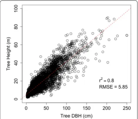
Field biomass estimation
as a linear function of DBH from all trees measured in the FIA dataset for Sonoma County for the 2001–2010 period (r2 = 0.8, RMSE = 5.85 m, Fig. 1).
We also tested the effects of omitting “cull” by substituting measured tree heights for predicted heights on estimates of county biomass totals, but found no substantial difference. The height prediction model occasionally over-predicted tree heights for large DBHs, when DBHs were outside the range used to calibrate the height model, and we adjusted overestimates by setting the maximum tree height to the maximum height found in each 30 m Lidar pixel. These tree height estimates, as well as tree species and DBH, served as inputs to the CRM estimates of tree biomass.
To estimate plot level biomass, we estimated a biomass density at the plot centroid by summing the biomass esti-mates for each tree, divided by the ‘plot area’ of that tree. Therefore each tree contributes to the biomass density of the plot centroid as a function of its biomass, and dis-tance from the plot centroid.
Lidar data
Wall-to-wall lidar data and high-resolution imagery were collected over Sonoma County in the summer of 2014. The lidar data were acquired at 900 m above ground with a field of view of 30°, with a nominal pulse density of 10.66 pulses/m2 at 105 kHz. We filtered lidar returns
to include only returns from vegetated surfaces. To accomplish this, a tree canopy mask was generated using high-resolution imagery and lidar using an object-based, data-fusion approach [17]. We used LAS tools software to extract vegetated lidar returns within 15 m of field plot centroids, and generate a suite of lidar metrics, includ-ing height percentiles, bincentiles (percentage of points
between the height cutoff and the maximum height), canopy cover and density, intensities and intensity per-centiles, and the quadratic mean lidar height of returns. A radius of 15 m was selected to approximately match the 30 m desired resolution of the county-wide map. We also tested using variable lidar radii to match the vari-able radius plots used in this study, but we found no sta-tistically significant improvement in model performance (Duncanson et al. in prep).
Biomass modeling
Random forest regression [1] was applied to model field biomass as a function of lidar metrics (described above) and ancillary metrics, including topography and spe-cies composition. We built three different random for-est models, one per allometric approach. We used the default random forest values of 500 trees, and 7 input variables (mtry = 7). We filtered outliers from the analy-sis that had lidar heights greater than 10 m, but a field biomass estimate of zero. We also filtered out four outli-ers that had small field biomass estimates (< 50 Mg/ha) but high lidar heights (> 30 m), assuming that these plot locations exhibited geolocation errors. We applied these two filters to remove obvious spatial outliers in the data-set where we think the forest canopy mask did not suffi-ciently remove vegetated returns from tall, non-vegetated surfaces (e.g. buildings). These two filters reduced our sample size from 179 to 166 plots.
Biomass mapping
We generated three maps of forest biomass density across the county, one for each set of allometric models. We esti-mated total aboveground biomass for the county and also divided pixels into discrete biomass density categories to assess the differences between allometric approaches in different biomass classes. We estimated the mean for the county by adjusting the mean pixel values to compensate for estimated deviation resulting from systematic model prediction error. We follow the model assisted regression estimator approach outlined by [16], to estimate both mean county biomass and also the standard error of the mean. We used a t test to assess whether county mean biomass estimates were statistically significantly different when using the different allometric models. A t test was selected both for simplicity and because the county-level biomass densities in forested areas of Sonoma County are approximately normal distributions (Fig. 9).
Results
Field biomass estimation
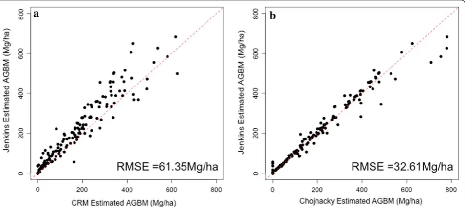
At a field plot level, the average biomass density estimates using the Jenkins et al. [12] method, the Chojnacky et al. [4] method, and the FIA’s CRM were 196.1, 195.8, and
164.9 Mg/ha, respectively. Although the average values for Jenkins and Chojnacky are statistically indistinguish-able, there is a 19% difference between those estimates and the FIA’s CRM. The difference between Jenkins esti-mates and CRM estiesti-mates is larger in plots with greater biomass values (Fig. 2a). Although the mean Jenkins and Chojnacky estimates match, the plot-level estimates differ appreciably, with Chojnacky estimating greater biomass density values in some high biomass plots (Fig. 2b). The distributions of field estimates from the three approaches show that the shape of the histogram of field plots is cap-tured by all three approaches, although again CRM pro-duces systematically smaller estimates (Fig. 3).
Biomass density modeling
We produced three models of biomass density, one per allometric approach. We found comparable model per-formance between the three allometric approaches, with the FIA’s CRM producing slightly higher correlations with lidar metrics than either the Jenkins or Chojnacky models (Fig. 4). The RMSE is also slightly lower for the FIA’s CRM, but the %RMSE is similar because of the 19% lower estimates. The %RMSE for Jenkins, Chojnacky, and FIA’s CRM are 46, 50, and 46%, respectively.
Of the 40 predictor variables, the percentile height met-rics were the most strongly correlated with above ground biomass. In particular, the lower relative height metrics were more sensitive to biomass (p10, p30, p40) than the higher height metrics. Additionally, the quadratic mean was a good predictor of forest biomass, followed by the
higher height percentiles. Indeed, all of the height per-centiles were more important predictors than any other variable, apart from the quadratic mean.
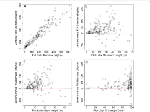
The relationship between Lidar and allometric variability Lidar-derived maximum height, mean height and % canopy cover were compared to discrepancies between the CRM and Jenkins estimates (Fig. 5). Addition-ally, residuals from the random forests models using the CRM and Jenkins biomass estimates were com-pared to both biomass and maximum forest height in an attempt to understand the drivers of allometric variability as well as the associated implications for biomass mapping (Fig. 6). There are clear patterns of overestimating low biomass densities and underes-timating high biomass densities exhibited in all three random forest models, although these patterns are relatively smaller using the CRM allometric estimates (Table 1). The largest deviations between allomet-ric estimates occurred in height ranges between 25 and 45 m, and the four tallest plots in the study area (height > 60 m) all had higher biomass estimates using the CRM approach. The largest discrepancies are not in the tallest forests, but in the 25–45 m forests with dense (> 80% cover) canopies and high estimated bio-mass density (Fig. 5). We focused on the discrepancies between CRM and Jenkins as these are the most popu-lar techniques applied, and there was no statistically significant difference between county-level estimates using Jenkins or Chojnacky models.
Biomass density mapping
Each of the three fixed radius biomass models was applied to the full suite of lidar and ancillary metrics for the county at a 30 m resolution. As with the models, the maps show the greatest discrepancies in areas of high biomass (Fig. 7) with Chojnacky predicting the larg-est high biomass values and the FIA’s CRM predicting the smallest. However, a relatively small fraction of the
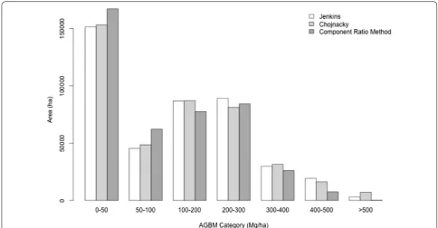
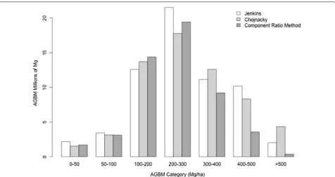
landscape exists as high biomass (< 4% by area > 400 Mg/ ha, Fig. 8), while the majority of Sonoma County’s land area falls either in low biomass (37% in < 50 Mg/ha) or mid-range biomass categories (39% in 100–300 Mg/ha).
The total biomass estimated for Sonoma County for the Jenkins, Chojnacky and CRM approaches was 62.17, 61.72, and 51.62 million Mg, respectively (Table 2). This represents less than 1% difference between the Jenkins
Fig. 3 The distribution of field estimates of biomass based on the three allometric approaches. The CRM produced lower estimates of biomass, vis-ualized here as greater numbers of field plots with AGBM < 200 Mg/ha, and fewer large biomass plots, while the Jenkins and Chojnacky approaches produced approximately the same number of estimates per biomass density category. In general, we sampled a larger number of low and medium biomass plots than high biomass plots in this study based on our stratified field sampling approach
and Chojnacky approaches, but a difference of 20.4% between the Jenkins and CRM methods, equating to a difference in 10.55 million tons of carbon. This differ-ence is caused primarily by lower predictions in the high biomass categories (Fig. 9). T tests of the model assisted estimates of the county means, using the model assisted estimators of county variances [16], revealed that the Jen-kins and Chojnacky estimates of mean county biomass are not statistically significantly different. Conversely, the CRM estimate of county mean is statistically significantly different (at 95% confidence) from both the Jenkins and Chojnacky estimates.
Discussion
Field estimates of aboveground biomass are often referred to as ‘ground truth’ data in remote sensing stud-ies, but without destructively sampling biomass in the field we do not know how accurate field estimates are. In this study, we demonstrate that allometric model
selection yields on average a 19% difference in field plot estimates of aboveground biomass, and a 20% difference in the resulting county-level biomass map for Sonoma County.
Sonoma County is a particularly interesting area to conduct this study, as it hosts forests with some of the highest biomass densities in the United States. We see that the majority of discrepancies between allometric predictions occur in these high biomass areas, which is expected because more trees with smaller stems are destructively sampled for allometric model fitting, and indeed published allometries are often caveated by unknown uncertainties above a certain stem girth [12]. For example, 91 of the trees in our field plots were larger than the largest tree destructively sampled in a respective species class, as reported by Jenkins, thus potentially con-tributing to greater errors for these 91 trees. Although these trees only represent 8% of those sampled across the county, they represent 18% of the total estimated biomass
in our field plots. However, given a lack of other available models, generalized allometric models such as applied in this paper are typically applied regardless of tree size.
The Jenkins and Chojnacky models were expected to perform similarly, as they are largely based on the same datasets of destructively sampled trees. The two stud-ies combined the meta-analysis differently, partition-ing allometric models from the literature into different combinations based on generalized species classes [12] or theoretical taxonomic groupings and wood specific gravity [4]. On average, these models produce similar biomass estimates and total county-level predictions, but discrepancies exist on a plot-to-plot basis depending on the species composition of a given plot. Most notably, the Chojnacky models produce greater estimates in high bio-mass plots, potentially because the models used by Cho-jnacky are more species-specific than the Jenkins models.
As with previous studies [4, 21], we found that the CRM field plot estimates were ~ 20% less than the Jen-kins predictions. In a similar analysis in Maryland, CRM estimates in FIA plots were only ~ 11% less than the Jen-kins estimates at the state level [11, 13]. The discrepancy between the differences seen in Maryland and Sonoma County could be due to the prevalence of conifer growth forms and larger trees found in Sonoma County, where we saw that estimates varied more in high biomass than low biomass areas.
There are several explanations for the differences between the Jenkins/Chojnacky and the CRM estimates seen both in this study and consistently observed in regional and national scale studies [5, 6, 14, 19]. First, the sample sizes used to construct the two sets of allometric models are different which could lead to systematic differ-ences. Duncanson et al. [3, 7] demonstrated that allometric
parameters are very sensitive to sample size, and that small sample sizes likely lead to an overestimate in biomass for a given DBH. The Jenkins and Chojnacky datasets are, on average, developed with smaller sample sizes than the FIA analysis [7]. These smaller sample sizes yield model devia-tions because of probable differences in the destructively harvested size distribution, with the inclusion likelihood of large individuals in a sample decreasing with sample size. Similarly, CRM volume models applied to certain species in Sonoma County were developed with destructively har-vested trees outside of the region, which may yield errors if trees in Sonoma County are growing in different climate conditions or have different resource limitations than those included in the sample [19].
Finally, others have suggested that the differences between Jenkins and CRM results are due to the inclu-sion of tree height in the CRM approach, which may bet-ter estimate stem volume. However, we do not see strong evidence of this here, as neither maximum nor mean lidar height were highly correlated to differences between CRM and Jenkins field estimates in the tallest forests in our study area. Indeed, the plots with maximum heights between ~ 25 and 45 m had the largest discrepancies, while the tallest trees sampled approached 70 m in height. This may suggest that Jenkins DBH-based estimates may be over estimating biomass in areas of moderate height (~ 25 m) and potentially underestimating biomass in tall forests (> 50 m), while CRM estimates constrain high predictions for a given DBH in relatively short forests and increase estimates for a given DBH in very tall forests. Notably, all of the plots with the highest discrepancies had > 80% canopy cover. As canopy cover is highly cor-related to biomass, it is unclear whether the variability in estimates is because of high canopy covers or high bio-mass densities. Certainly the limited destructive sample for large tree sizes would explain the high biomass den-sity discrepancies, but it is conceivable that destructively harvested trees were also preferentially extracted from open, easily accessible areas with lower canopy covers. This may have caused deviations in allometries in com-parison to trees growing in closed canopy systems with relatively taller, smaller crowned individuals.
Our assessment of the drivers of variability between allometric model selection remains speculative. We see that discrepancies are largest in high biomass plots with high canopies covers and moderate heights. Whether these discrepancies are due to inadequate sampling across gradients of biomass, canopy cover or height in either CRM, Jenkins/Chojnacky, or all datasets remains uncertain. Only testing the different allometric approaches against an independent destructively sampled
Table 1 Average residuals per height and biomass class using the CRM and Jenkins approaches show that while both approaches overestimate low biomass and under-estimate high biomass the Jenkins model has a slightly higher overall deviation as well as markedly higher over-estimates in low-moderate biomass plots. This trend is not apparent with respect to height class
CRM Jenkins n
0–10 m 4.26 8.25 35
10–25 m 3.24 6.58 66
25–40 m 6.09 − 5.01 43
40–55 m − 11.81 − 0.27 18
> 55 m − 56.19 7.5 4
Total 1.2 2.98 166
0–100 Mg/ha 22.7 33.7 71
100–200 Mg/ha 40.44 52.1 36
200–300 Mg/ha − 6.89 12.03 25
300–400 Mg/ha − 59.35 − 75.95 21 > 400 Mg/ha − 111.55 − 88.37 13
Total 1.2 2.98 166
tree dataset can determine the underlying drivers, and such a dataset is currently unavailable for use in this study. However, these results highlight the importance of improving allometric models for biomass mapping. Fortunately, progress is being made in this field, both through the collection of larger destructively harvested tree datasets that can be used to fit improved models (e.g. [5] or through the derivation of new, non-destructively derived allometries based on terrestrial laser scanning (TLS)(e.g. [2]).
Conclusions
All empirically derived aboveground biomass estimates are fundamentally based on the application of allomet-ric models in the field, and thus have an error that is often unknown and unreported. The allometric models
used in this study showed an approximately 20% dif-ference in both mean plot-level and county-level totals of estimated aboveground biomass. This 20% differ-ence is not a 20% error, as we do not have direct field measurements of biomass. Indeed, the error in field biomass estimation is likely to be greater than 20%, particularly in high biomass forests such as exhibited in some areas of Sonoma County. We found the larg-est discrepancies between allometric field larg-estimates in high biomass plots with heights between 25 and 45 m, with > 80% canopy cover. Lidar heights were not highly correlated to discrepancies amongst popular allomet-ric approaches, suggesting that an incorporation of height into models is unlikely to fully resolve observed discrepancies.
Fig. 8 Biomass density distributions by area. Sonoma County is dominated by small biomass areas, with < 4% of the area predicted to have bio-mass densities > 400 Mg/ha
Table 2 Plot and county based statistics describing differences between the three different allometric approaches for plot-level biomass estimation. Total and Mean county estimates are based on map pixels alone, while the model assisted (MA) estimates have been adjusted to compensate for estimated deviation resulting from systematic model pre-diction (map) error
Total county
(mil-lion Mg) Mean county (Mg/ha) Mean county (MA, Mg/ha) SE of mean (MA, Mg/ha) Mean plot (Mg/ha) SE residuals (Mg/ha)
Jenkins 62.17 147.8 145.2 7.13 199.2 78.54
Chojnacky 61.72 146.8 143.7 7.73 199.02 85.4
We anticipate many of existing problems related to forest biomass allometry will be addressed by the grow-ing popularity of TLS, which enables field measurement to expand past stem diameters and heights to include full tree volumes. Taken in combination with traditional mensuration, this technology can either directly replace field estimates of biomass through direct estimation of individual tree volumes at the plot level, or improve existing allometric models through the inclusion of much greater numbers of non-destructively sampled individuals.
The findings in this not only underscore the impor-tance of allometry in forest biomass mapping, but high-light that errors in existing allometric models are poorly understood. Further research into the effects of sample size, geographic representativeness, functional form, and the utility of TLS to address these questions is required to properly characterize errors in field estimates of bio-mass, and propagate these errors through to maps. This is particularly timely considering several upcoming active remote sensing datasets that will be used to map forest biomass at a global scale (e.g. NASA’s GEDI, NISAR, ESA’s BIOMASS). As in this study, the quality of these global maps will depend on the quality of field data used to calibrate the associated empirical biomass models, which will necessarily depend on the accuracy of the
underlying allometric models. Thus, forest allometry is not only important at the local–regional scale studies in this paper, but for carbon accounting at a global scale.
Authors’ contributions
LD designed the study, conducted the statistical analysis and wrote the paper. WH and LD processed the lidar data, and WH generated the biomass maps. KJ calculated the CRM allometric estimates. RM assisted in statistical analysis of county-level estimates. AS and RD managed the generation of the empirical biomass maps for Sonoma County. All authors assisted in writing the manu-script. All authors read and approved the final manumanu-script.
Author details
1 Biosciences Laboratory, NASA Goddard Space Flight Center, Greenbelt, USA. 2 Department of Geographical Sciences, University of Maryland, College Park,
USA. 3 USDA Forest Service, Northern Research Station, Newton Square, PA,
USA. 4 USDA Forest Service, Northern Research Station, Saint Paul, MN, USA.
Acknowledgements
The authors gratefully acknowledge Aaron Arthur and Amanda Whitehurst for collection of field data, Mark Tukman for helping manage field data collection, and Jarlath O’Neill Dunne for processing the 1 m forest/non-forest mask. Additional thanks go to NASA’s Carbon Monitoring System for supporting this work.
Competing interests
The authors declare that they have no competing interests. Additional file
Availability of data and materials
The lidar data used in this study will be available on the Oak Ridge DAAC approximately 1 month after the submission date, therefore a link to the lidar dataset will be included here prior to submission. All Forest Inventory Analysis data used to fit diameter to height models are available online at http://www. fia.fs.fed.us/.
Consent for publication
Not applicable.
Ethics approval and consent to participate
Not applicable.
Funding
This work was funded by NASA’s Carbon Monitoring System Grants NNH12AU32I, PI Dubayah and NNH15ZDA001N.
Publisher’s Note
Springer Nature remains neutral with regard to jurisdictional claims in pub-lished maps and institutional affiliations.
Received: 9 June 2017 Accepted: 7 October 2017
References
1. Breiman L. Random forests. Mach Learn. 2001;45(1):5–32. 2. Calders K, Newnham G, Burt A, Murphy S, Raumonen P, Herold M,
Kaasalainen M. Nondestructive estimates of above-ground biomass using terrestrial laser scanning. Methods Ecol Evol. 2015;6(2):198–208. 3. Chave J, et al. Improved allometric models to estimate the aboveground
biomass of tropical trees. Glob Chang Biol. 2014;20(10):3177–90. 4. Chojnacky DC, Heath LS, Jenkins JC. Updated generalized biomass
equa-tions for North American tree species. Forestry. 2014;87(1):129–51. 5. Clough BJ, Russell MB, Domke GM, Woodall CW. Quantifying allometric
model uncertainty for plot-level live tree biomass stocks with a data-driven, hierarchical framework. For Ecol Manage. 2016;372:175–88. 6. Domke GM, Woodall CW, Smith JE, Westfall JA, McRoberts RE.
Conse-quences of alternative tree-level biomass estimation procedures on US forest carbon stock estimates. For Ecol Manage. 2012;270:108–16. 7. Duncanson L, Rourke O, Dubayah R. Small sample sizes yield biased
allo-metric equations in temperate forests. Scientific Reports. 2015;5:17153. 8. Gibbs HK, Brown S, Niles JO, Foley JA. Monitoring and estimating
tropical forest carbon stocks: making REDD a reality. Environ Res Lett. 2007;2(4):045023.
9. Goetz SJ, Baccini A, Laporte NT, Johns T, Walker W, Kellndorfer J, Houghton RA, Sun M. Mapping and monitoring carbon stocks with satellite observations: a comparison of methods. Carbon Balance Manag. 2009;4(1):2.
10. Heath LS, Hanson MH, Smith JE, Smith WB, Miles PD. Forest inventory and analysis (FIA) symposium 2008. In: McWilliams W, Moisen G, Czaplewski R, (editors.), Investigation into calculating tree biomass and C in the FIADB using a biomass expansion factor approach. 2009, USDA For. Serv. Proc. RMRS-P-56CD.
11. Huang W, Swatantran A, Johnson K, Duncanson L, Tang H, O’Neil Dunne J, Hurtt G, Dubayah R. Local discrepancies in continental scale biomass maps: a case study over forested and non-forested landscapes in Maryland, USA. Carbon Balance Manag. 2015;10:19. doi:10.1186/ s13021-015-0030-9.
12. Jenkins JC, Chojnacky DC, Heath LS, Birdsey RA. National-scale biomass estimators for United States tree species. For Sci. 2003;49(1):12–35. 13. Johnson KD, Birdsey R, Finley AO, Swantaran A, Dubayah R, Wayson C,
Rie-mann R. Integrating forest inventory and analysis data into a LIDAR-based carbon monitoring system. Carbon Balance Manag. 2014;9(1):3. 14. MacLean RG, Ducey MJ, Hoover CM. A comparison of carbon stock
estimates and projections for the northeastern United States. For Sci. 2014;60(2):206–13.
15. Matyas WJ, Parker I. CALVEG mosaic of existing vegetation of California. San Francisco: Regional Ecology Group, US Forest Service, Region 5; 1980. 16. McRoberts RE, Cohen WB, Næsset E, Stehman SV, Tomppo EO. Using
remotely sensed data to construct and assess forest attribute maps and related spatial products. Scand J For Res. 2010;25(4):340–67. doi:10.1080/ 02827581.2010.497496.
17. O’Neil-Dunne JP, MacFaden SW, Royar AR, Pelletier KC. An object-based system for LiDAR data fusion and feature extraction. Geocarto Int. 2013;28(3):227–42.
18. Pan Y, Birdsey RA, Fang J, Houghton R, Kauppi PE, Kurz WA, Phillips OL, Shvidenko A, Lewis SL, Canadell JG, Ciais P, Jackson RB, Pacala SW, McGuire AD, Piao S, Rautianinen A, Sitch S, Hares D. A large and persistent carbon sink in the world’s forests. Science. 2011;333(6045):988–93. 19. Westfall JA. A comparison of above-ground dry-biomass estimators for
trees in the northeastern US. North J Appl For. 2012;29(1):26–34. 20. Woodall C, Heath LS, Domke GM, Nichols MC. Methods and equations for
estimating aboveground volume, biomass, and carbon for trees in the US forest inventory, 2010. USDA: US Forest Service; 2011.
21. Zhou X, Hemstrom MA (2009) Estimating aboveground tree biomass on forest land in the Pacific Northwest: a comparison of approaches. Res. Pap. PNW-RP-584. Portland: US Department of Agriculture, Forest Service, Pacific Northwest Research Station.