CROSS SECTIONS USED TO ELUCIDATE DIFFERENCES IN WAVELET TRANSFORMS
OF GROUND FORCE REACTIONS
by
Wesley John Orme
A thesis
submitted in partial fulfillment of the requirements for the degree of Master of Science in Mechanical Engineering
Boise State University
BOISE STATE UNIVERSITY GRADUATE COLLEGE
DEFENSE COMMITTEE AND FINAL READING APPROVALS
of the thesis submitted by
Wesley John Orme
Thesis Title: Cross Sections Used to Elucidate Differences in Wavelet Transforms of Ground Force Reactions
Date of Final Oral Examination: 15 October 2009
The following individuals read and discussed the thesis submitted by student Wesley John Orme, and they evaluated his presentation and response to questions during the final oral examination. They found that the student passed the final oral examination.
Joseph Guarino, Ph.D. Chair, Supervisory Committee Robert Hamilton, Ph.D. Member, Supervisory Committee Michelle Sabick, Ph.D. Member, Supervisory Committee
ii DEDICATION
iii
ACKNOWLEDGEMENTS
First, great thanks to my advisor, Dr. Guarino, committee members Dr. Hamilton and Dr. Sabick, and Wayne Fischer for the continued support, motivation, editing, and input. Projects such as these are much easier with great support groups.
Also, thank you to the following individuals from Boise State University for setting up the single leg unanticipated drop landing experiment, gathering the data, and
iv
AUTOBIOGRAPHY
My education and career have been widely varied as I have always enjoyed the adventure of learning and trying something new. Upon graduation from high school, I enrolled in the Automotive Engineering Technology at Ricks College (now Brigham Young University Idaho) and, after a year, switched programs and graduated with an Associate’s degree in Manufacturing Engineering Technology in May of 1992. After spending several years in the manufacturing and construction industries, I enrolled in the Mechanical Engineering program at Boise State University where I graduated with a Bachelor’s of Science degree in May of 2003. Shortly after graduation, I started taking classes in pursuit of a Master’s of Science degree with an emphasis in dynamics and systems analysis.
My engineering career has been focused on mechanical design and data analysis. In my current position, I analyze mechanical failures due to vibrations, impacts, and
environmental conditions and provide design feedback to the original equipment manufacturers.
The subject of this thesis allowed me an opportunity to learn new methods of
v ABSTRACT
A study done for the Centers for Disease Control (CDC) found that over 50% of sports related injuries are to the lower extremities [1] with additional studies indicating that females, adolescent through collegiate, have a higher rate of lower extremity sports related injuries than males [2-4]. Conditions surrounding non-contact injuries can be analyzed using ground reaction force (GRF) data from force plates during unanticipated single leg drops, however, the expected gender differences in GRF may not be apparent when viewing data independently in the time or frequency domains.
Graphing the results of a wavelet transform, currently used by scientific, medical, and financial communities [5], allows simultaneous viewing of time, frequency, and magnitude data. In this case, the wavelet transform was chosen over the Short Time Fourier Transform as it is better suited for analyzing transient or aperiodic signals.
The differences in the transformed signals were subtle therefore, further steps were taken to further elucidate the differences. In previous studies coherence between the two matrices (in this case, male and female) was calculated and graphed [6, 7]. The method proposed in this thesis utilizes the coherence method to determine the regions of greatest difference then, a slicing technique is used to view differences at specific frequencies.
vi
forces and Z axis moments (about the vertical axis). The greatest differences are shown in the X and Y forces and the moments about the Z axis. In previous studies, due to the magnitude of the forces, the focus was on the Z axis reaction forces. Results of this thesis imply that future studies should also consider on the moments and the reaction forces of the X and Y axes. The results of this thesis combined with studies showing that the frequencies of maximum transmissibility of the lower extremity muscles are less than 50 Hz [8] and the resonant frequencies of the patellar tendon are between 22 and 25 Hz [9], imply that the gender differences seen at low frequencies may correlate with the difference in injury rates.
vii
TABLE OF CONTENTS
DEDICATION ... ii
ACKNOWLEDGEMENTS ... iii
AUTOBIOGRAPHY ... iv
ABSTRACT ... v
LIST OF TABLES ... x
LIST OF FIGURES ... xi
LIST OF EQUATIONS ... xiv
INTRODUCTION ... 1
Motivation ... 1
Objective ... 2
HYPOTHESIS ... 3
LITERATURE REVIEW ... 4
Principles and Methods of Wavelet Transforms ... 4
Applications of Wavelets ... 7
Evaluations of Landings from Drops and Jumps ... 8
Gender Differences in Sports Injury Rates ... 9
Audio Comparison of Signals ... 10
DATA PROTOCOL ... 11
Unanticipated Drop Protocol ... 11
viii
Instrumentation ... 13
Data Preperation Protocol ... 14
Data Averaging Protocol ... 16
Data Exclusion Protocol ... 16
DATA ANALYSIS USING WAVELET TRANSFORMS ... 17
Time Based Analysis ... 17
Frequency Based Analysis ... 19
Wavelet Based Analysis ... 19
Wavelet Statistics ... 20
Wavelet Coherence ... 22
Wavelet Slicing Analysis ... 23
AUDIO ANALYSIS ... 25
CSV Conversion ... 25
Audio Transformation ... 26
CONCLUSIONS... 27
Wavelet Transform Analysis ... 27
Audio Analysis ... 27
Significance ... 27
Future Studies ... 28
REFERENCES ... 30
ix
APPENDIX B ... 39 Fourier Transforms of Averaged SignalsFigure
APPENDIX C ... 44 Wavelet Transforms with Statistics
APPENDIX D ... 49 Cross Wavelet Coherence Phase
APPENDIX E ... 52 Wavelet Cross Sections
APPENDIX F... 57 Pitch Shifted Audio Spectrums of Force Plate Reactions
x
LIST OF TABLES
xi
LIST OF FIGURES
Figure 1: Comparison by Gender of Sports Related Injuries ... 2
Figure 2: Occurrences of Sports Related Injuries ... 2
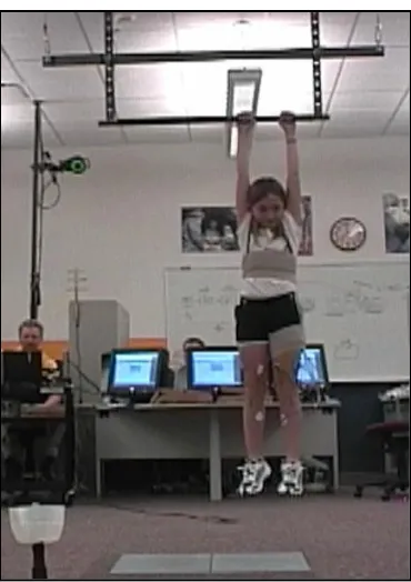
Figure 3: Female Subject Preparing for Unanticipated Drop Landing ... 12
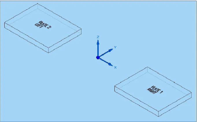
Figure 4: Force Plate Layout and Axes... 13
Figure 5: All Signals as Recorded ... 14
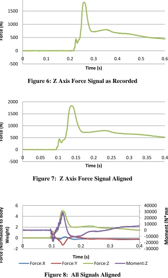
Figure 6: Z Axis Force Signal as Recorded ... 15
Figure 7: Z Axis Force Signal Aligned ... 15
Figure 8: All Signals Aligned ... 15
Figure 9: Aligned Mean Z Axis Reaction Force Signal ... 18
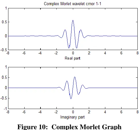
Figure 10: Complex Morlet Graph ... 20
Figure 11: Example of a Wavelet Transform with Statistics ... 21
Figure 12: Example of Coherence Phase ... 23
Figure 13: Example of a Z Force Wavelet Slice at 25 Hz ... 24
Figure 14: Audio Signal Modifications ... 26
Figure 15: Mean Transmissibility of Lower Extremity Muscles ... 28
Figure A.1: X Force Left / Right Leg Time Domain ... 35
Figure A.2: Y Force Left / Right Leg Time Domain ... 36
Figure A.3: Z Force Left / Right Leg Time Domain ... 37
Figure A.4: Z Moment Left / Right Leg Time Domain ... 38
xii
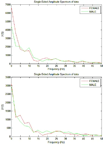
Figure B.2: Y Force Left / Right Leg Frequency Domain ... 41
Figure B.3: Z Force Left / Right Leg Frequency Domain ... 42
Figure B.4: Z Moment Left / Right Leg Frequency Domain ... 43
Figure C.1: X Force Left Leg Wavelet Transforms ... 45
Figure C.2: X Force Right Leg Wavelet Transforms ... 45
Figure C.3: Y Force Left Leg Wavelet Transforms ... 46
Figure C.4: Y Force Right Leg Wavelet Transforms ... 46
Figure C.5: Z Force Left Leg Transforms ... 47
Figure C.6: Z Force Right Leg Wavelet Transforms ... 47
Figure C.7: Z Moment Left Leg Wavelet Transforms ... 48
Figure C.8: Z Moment Left Leg Wavelet Transforms ... 48
Figure D.1: X Force Left/Right Leg Coherence Phase ... 50
Figure D.2: Y Force Left/Right Leg Coherence Phase ... 50
Figure D.3: Z Force Left/Right Leg Coherence Phase ... 50
Figure D.4: Z Moment Left/Right Leg Coherence Phase ... 51
Figure E.1: X Force Left Leg Slices ... 53
Figure E.2: X Force Right Leg Slices ... 53
Figure E.3: Y Force Left Leg Slices ... 54
Figure E.4: Y Force Right Leg Slices ... 54
Figure E.5: Z Force Left Leg Slices ... 55
Figure E.6: Z Force Right Leg Slices ... 55
Figure E.7: Z Moment Left Leg Slices ... 56
xiii
Figure F.1: X Force Left Leg Audio Signals ... 58
Figure F.2: X Force Right Leg Audio Signals ... 58
Figure F.3: Y Force Left Leg Audio Signals ... 59
Figure F.4: Y Force Right Leg Audio Signals ... 59
Figure F.5: Z Force Left Leg Audio Signals... 60
Figure F.6: Z Force Right Leg Audio Signals ... 60
Figure F.7: Z Moment Left Leg Audio Signals ... 61
xiv
LIST OF EQUATIONS
INTRODUCTION
Studies analyzing the landing phase of jumps and drops, both single leg and bilateral, have been utilized to gather data of the events surrounding non contact sports injuries. Information gathered from these landings have included reactions from force plates [10-12], angles of joints such as the hips and knees [3, 4, 13-15], measures of joint kinematics such as acceleration [16], and muscle activity [8, 17]. The desired result of these studies was to determine how injuries occur or quantify the differences between participating groups.
Motivation
Figure 1: Comparison by Gender of Sports Related Injuries
Figure 2: Occurrences of Sports Related Injuries
Objective
HYPOTHESIS
LITERATURE REVIEW
The literature search was divided into five sections including principles and methods of wavelet transforms, applications of wavelet transforms, evaluations of landings from drops and jumps, differences between genders in sports injury rates, and the use of audio to compare signals.
Principles and Methods of Wavelet Transforms
This section of the literature search focused on the definition of a wavelet, wavelet functions, and the options within the wavelet function.
The wavelet transform is used to view the frequency and magnitude information of a signal with respect to time. The concept of the wavelet transform is similar to the Short Time Fourier Transform with a specific function (mother wavelet) being used in place of the sine and cosine functions to transform the signal into the frequency domain with respect to time.
When using the Morlet mother wavelet, several options, settings, and limitations need to be considered. The following paragraphs will show the rationale for these decisions.
The need for real and imaginary components of the transform to compute the
coherence and phase angle lead to the decision to use the complex Morlet Transform [6]. The transform can be either discrete or continuous. Discrete transforms analyze the signals in sections and are used for space saving coding or when there is a need to reconstruct the signal. Continuous transforms consider the entire signal and are used to make traits of the transform more visible in graphs. As the graphs were to be considered and the signal did not need to be reconstructed, the continuous transform was chosen [18].
Two settings within the Morlet Transform are center frequency and bandwidth. Both are used to adjust the shape of the mother wavelet. When differences between the
transforms of two signals are to be considered, the same mother wavelet is applied to both signals. It was found that these settings did not change the resulting differences therefore, for ease of calculating the real frequency; both were set to 1 Hertz [18].
The scaling factor is chosen based on the level of detail required and the
The Complex Morlet mother wavelet has a simplified form which is commonly used for the transform. This simplification results in invalidation of the transforms below 5.4 Hertz. The simplified equation is used by Matlab therefore; the transforms in this analysis are a result of the simplified equation [5].
Validation of the transforms needs to be done to eliminate two sources of error, edge effects and noise. The cone of influence outlines the area which is subject to edge effects which may generate false frequencies [6]. Significance testing was initially used by Torrence and Campo but, Ge, citing errors with the Monte Carlo simulation, suggested using white noise for the basis of the significance testing [19].
After the transforms are complete and verified, they can be compared utilizing the real and imaginary components of the transform and generating coherence and phase angle plots. These plots will give the location with respect to frequency and time where the two transforms are most and least different [7].
Once the signals used for this thesis were processed using the methods above, the areas of difference were identified but, not clear in the graphs of the wavelet transforms. The method of slicing the wavelet transform matrices in the areas of difference has not been previously documented in a study.
As a result of this literature search, the transforms of this data was done with a simplified form of the complex, continuous Morlet mother wavelet with a scaling factor of 128 and a center frequency and bandwidth setting of 1 Hertz. The transforms were then subjected to validation to eliminate edge effects and noise as sources of error.
Applications of Wavelets
Applications of wavelet transforms can be found in science, engineering, finance, and medicine “for analyzing signals which and be described as aperiodic, noisy,
intermittent, transient, and so on” [5]. The articles listed in Table 1 are some examples of wavelet uses:
Table 1: Applications of Wavelet Transforms, Literature Search Results
Article Title Profession Short Description Reference Cross-Correlation Analysis of Epileptiform Propagation Using Wavelets Medical
Wavelets are used to transform electrical signals from different
parts of the brain. Cross correlation used to determine
the relationship between the different parts of the brain.
[20] Comparing Time Series Using Wavelet Based Semblance Analysis Geophysics
Wavelets are used to transform synthetic signals with cross
correlation demonstrated.
[21]
A Practical Guide to Wavelet
Analysis
Geophysics Wavelet transformation of
oceanic signals [6]
Vibes Scope
Machine Health Engineering
Wavelet transforms of vibration measurements from rotating
equipment.
[22] Application of the
Cross Wavelet Transform and Wavelet Coherence to Geophysical Time Series
Geophysics Wavelet transformation of
oceanic signals [7]
A search for studies in which wavelet transforms were used to analyze GRF yielded no articles.
Evaluations of Landings from Drops and Jumps
The initial intent of this section of the literature search is to aid in understanding the protocols, expected results, and methods of analysis used for evaluating drop jumps. During this research, some articles referring to the resonant frequencies of tissues and their relationship to damage caused an expansion of the search criteria as this relationship adds motivation to the study.
The results of this search will be reported in the categories of types of sensors used, gender differences, fatigue, and resonant frequencies of tissues.
The studies that focused on ground reaction forces (GRF) either independently or correlating to landing mechanics used force plates to record the ground reaction forces. Other equipment used included accelerometers and cameras recording positions of reflective targets. As a result, it can be concluded that recording GRF from drops (either unanticipated or from a jump) using force plates is an accepted method for studying the landing techniques of athletes [12, 14-16, 23].
Differences between genders in landing mechanics was a common study with the differences occurring in age, type of jump or landing, and the data recorded. While the studies and outcomes were varied, the commonality between the studies was the premise that landing mechanics could have an effect on injury rates [10, 15, 17, 24-26].
done on males only, the results indicate that single leg drops are more reliable for prognostic and diagnostic information than jumps [23]. The height in this study was controlled to eliminate jump height as a variable.
The effect of fatigue on landing mechanics has also been studied. At first glance, the results are mixed with one study reporting fatigue affects landings and another reporting the opposite. Upon closer inspection, fatigue affects landings from jumps [13] and does not affect landings from drops [14]. To err on the side of caution, the number of trials used in this analysis was limited to 10 per leg to eliminate the potential effects of fatigue.
There are theories that maximum tissue damage occurs when the force is applied at the resonant frequency. The resonant frequency for some muscles and tendons of the lower extremities is below 50 Hz [8, 9]. Finding the resonant frequency of the muscles, tendons, and bones indicates that the analysis should focus on frequencies lower than 50 Hz.
Gender Differences in Sports Injury Rates
Although many of the articles found in during the evaluations of landings from drops and jumps literature search cited differences in injury rates, a specific search for gender differences in sports injury rates yielded only two articles, “Epidemiology of Collegiate Injuries for 15 Sports: Summary and Recommendations for Injury Prevention Initiatives” and “Injury and Disability in Matched Men’s and Women’s Intercollegiate Sports” [2].
in injury rates were not discussed. However, from the graphs shown, higher injury rates were not consistent relative to gender. The information from this study that helped with the motivation of this thesis is the fact that over fifty percent of the injuries are in the lower extremities (see Figure 2) [1].
The second study was done at a single university for the period of one year. Injury rates for eight matched sports were found to be similar with the exception of gymnastics where the female injury rate was much higher per hour of exposure. One method of grouping the injuries from the eight matched sports showed that, in general, females had a higher injury rate to the lower extremity than males (see Figure 1) [2].
The two studies yielded the following: One conclusion to be drawn is that the female injury rate is not always the highest when considering matched sports. The second conclusion is due to the low occurrence of injuries, the sample size must be large to ensure accuracy.
Audio Comparison of Signals
Most studies involving audio comparison of signals gather data with microphones and analyze frequency content. However, there is a study titled “Multimodal Motion Processing in Area V5/MT: Evidence from an Artificial Class of Audio-Visual Events” [27] in which GRF data signals from counter movement jumps were converted to an audio signal, modified, then used in their experiment. The audio modifications modulated “frequency and amplitude of the standard pitch “A” (440 Hz).
DATA PROTOCOL
The following section describes the processes used to gather, prepare, and analyze the forces and moments measured by the force plates during the unanticipated single leg drop landings.
Unanticipated Drop Protocol
Figure 3: Female Subject Preparing for Unanticipated Drop Landing
The data for this thesis is extracted from the landing phase of the trials done for “Effect of Gender on Lower Extremity Muscle Activation in Children Performing A Single-Leg Unanticipated Landing Task” at Boise State University [10]. During the trials, the subject was given a signal during freefall, to cut left, right, or run straight forward. The "cutting" portions of the signals were not analyzed nor were the landings categorized by the direction of the cut. As this thesis is focused on a method for determining differences, this should not affect the results of the analysis.
The subjects participated in several landings on each leg. In an effort to eliminate fatigue as a factor, only the first 10 trials of each leg from each subject were used.
Subject Demographics
Table 2: Subject Demographics
Males Females
Value Standard Deviation Value Standard Deviation
Number of Subjects 17 N/A 21 N/A
Average Age (years) 10.44 0.63 10.05 0.69
Average Height (m) 1.44 0.08 1.45 0.08
Average Weight (N) 354.5 53.7 363.9 79.0
Instrumentation
The force plates and data acquisition software are manufacutured by Kistler Instruments. The force plates, positioned as seen in Figure 4, are model number 9281C with a natural frequency of 1000 Hz [28]. The data acquisition software, BioWare™, was set up to sample the data at a rate of 1250 Hz [29].
The data was output in a .csv format with all of the forces and moments for the trial in separate columns. Each trial was recorded in a separate file.
Data Preperation Protocol
When comparing wavelet transforms, care must be taken to align the time based signal to a common reference point while ensuring that the data of interest is far enough from the end of the file to prevent the influence of edge effects during the transform. For this purpose, a program was written in LabVIEW™ to perform the following functions [30].
The first step was to validate the data using the Z axis force. The first criterion ensured that the maximum value was greater than twice the subjects body weight to ensure that a landing was recorded in the data file. The second criterion ensured that the first reading greater than 30 Newtons was at the 120th (0.1 seconds) data point greater.
The next step was to remove data points pre and post impact so that the first data point in the Z axis force greater than 30 Newtons was the 120th data point and the final data point was 500th (0.4 seconds). This was done to all of the forces and moments associated with that trial to maintain alignment with the Z axis force. The initial anaylsis was done by aligning the peak Z axis forces, however it was found that the point of initial contact or 30 Newton point was more reliable.
Figure 5: All Signals as Recorded
-30000 -20000 -10000 0 10000 20000 30000 40000 -1000 -500 0 500 1000 1500 2000
0 0.2 0.4 0.6
Fo rc e (N ) Time (s)
Force:X Force:Y Force:Z Moment:Z
Figure 6: Z Axis Force Signal as Recorded
Figure 7: Z Axis Force Signal Aligned
Figure 8: All Signals Aligned -500 0 500 1000 1500 2000
0 0.1 0.2 0.3 0.4 0.5 0.6
Fo rc e (N ) Time (s) -500 0 500 1000 1500 2000
0 0.05 0.1 0.15 0.2 0.25 0.3 0.35 0.4
Fo rc e (N ) Time (s) -30000 -20000 -10000 0 10000 20000 30000 40000 -2 0 2 4 6
0 0.1 0.2 0.3 0.4
Fo rc e (N o rm al ize d t o B o d y Wei gh t) Time (s)
Force:X Force:Y Force:Z Moment:Z
The final steps in this program normalized the forces to the subjects body weight and parsed the forces and moments of the individual axes into separate files.
Data Averaging Protocol
There is not a standard landing GRF signal for males or females to which individual signals can be compared. For this thesis, it was decided that comparing a single averaged signal from each gender would allow the demonstration of proposed technique. The first 10 trials from all subjects of a gender were averaged resulting in a single force and moment signal for each axis, leg, and gender.
Data Exclusion Protocol
DATA ANALYSIS USING WAVELET TRANSFORMS
To establish and illustrate the need for using slices of wavelet transforms to view differences, the signals from the forces and moments are shown in three different ways. The time based signals show the magnitudes of forces and moments as they were recorded. A Fourier Transform was performed on the time based signals to view the magnitude of each frequency. Wavelet transforms, coherence, and slices were then used to isolate specific frequency content with respect to time.
Time Based Analysis
The time based signals shows the magnitude of each force and moment as it occurs in time. This force plate reaction data was recorded by BioWare™ and stored in .csv files.
Figure 9: Aligned Mean Z Axis Reaction Force Signal
Graphs of the manipulated individual time based signals may be viewed in Appendix A.
For the discussion regarding the time based signals as well as the other graphs, the comments will be focused on the differences. When comparing the manipulated time based signals from each gender for each leg in the different axes, it is best to focus on the shape, maxima, and the maxima location of each signal with respect to time.
An inspection of the graphs in Appendix A yields some differences between the genders in the averaged data. The largest percent difference can be seen in the Y axis forces where the magnitude of the female signal is greater than the male at the time corresponding with the maximum reaction point in the Z axis. Another area of difference can be seen in the Z axis where the magnitude of the male signal is greater at the toe on point and the magnitude of the female signal is greater at the maximum reaction point.
A statistical t-test performed on the peak Z axis forces for both the left and right legs indicates that it is likely that the average male and female and female forces are the same. The t-statistic for the left leg samples is 0.9538 and the right leg is -0.0454. The 80%
TOP (~0.12 s) MRP (~0.18s)
confidence interval for this size of sample is 1.2816 which indicates the similarities of the forces [31].
While there are some differences in the time based signals, current studies noting the tissue damage due to the frequency content of the signal lead to the next step of analyzing the signals in the frequency domain.
Frequency Based Analysis
Transforming the time based signals into the frequency domain was done using a program in Matlab and utilizing the Fourier Transform [18]. All frequencies above 50 Hz were very similar and current studies indicate that muscle damage occurs below 50 Hz therefore, the frequency scale of the graphs was limited to 50 Hz. The resulting graphs may be seen in Appendix B.
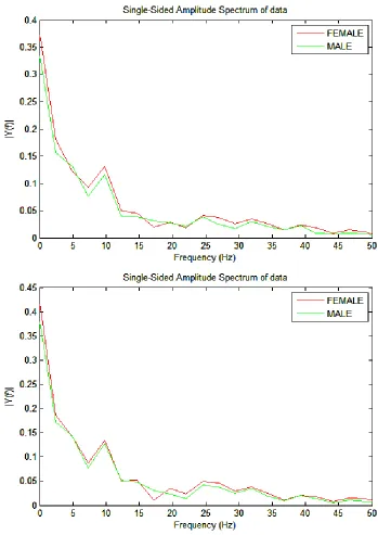
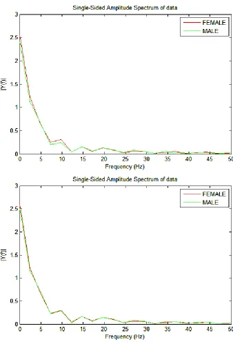
In general, the Fourier Transforms of the force signals from each gender are similar in shape and magnitude with the maxima occurring at less than 5 Hz and some
differences in magnitude of individual frequencies.
Viewing the signals in the frequency domain shows only that the frequency reaches maximum amplitude somewhere in time. The wavelet transform will show details of magnitude and frequency with respect to time.
Wavelet Based Analysis
As previously noted in the literature search, impact signals are best transformed using the Morlet or Complex Morlet mother wavelet [5]. For this analysis, the
[18] was chosen with a scaling factor of 128, center frequency (fc), and a bandwidth
frequency (fb) of 1 Hz.
𝝍 𝒙 =
𝟏
𝝅𝒇
𝒃𝒆
𝟐𝒊𝝅𝒇𝒄𝒙𝒆
−𝒙𝟐
𝒇𝒃
Equation 1: Simplified Complex Morlet Equation
Figure 10: Complex Morlet Graph
While fine tuning the transform process, analysis of the only the real portion of the signal was considered. While the real portion of the transform appeared to be an accurate representation of the signal, using the power of the wavelet transform (squaring the absolute value of the real and imaginary parts) amplified the differences in gender.
Wavelet Statistics
[6] which has been compared to “slamming a door shut” on the analysis resulting in the generation of false frequencies. Other authors have used significance testing to ensure the data shown was not due to noise in the time based signal by comparing the transforms to different types of noise (i.e. red noise, white noise, etc.) [19]. In this thesis, the signal was compared to white noise (consistent power level through the entire spectrum) with a confidence interval of 95%. For the following graphs, the red parabolic line denotes the Cone of Influence and the black lines denote the significance levels.
The wavelet transforms and statistical analysis were completed using programs written in Matlab and the resulting graphs may be seen in Appendix C.
Figure 11: Example of a Wavelet Transform with Statistics
The resulting graphs of the wavelet transforms show differences in magnitude and frequency with respect to time. With close inspection of the wavelet transform graphs in Appendix C, the reader will note that there are some differences in magnitude and the maxima are slightly shifted in time. With better resolution (more steps), gradients would become more defined and differences would be more obvious.
Area within the Cone of Influence Area eliminated by Significance
Wavelet Coherence
Wavelet coherence begins with a method commonly used to compare two matrices with real and imaginary components as described in Equation 2. Torrence and Campo called this computation the cross wavelet spectrum [6].
𝑊
𝑛𝐹(𝑠) ≡ 𝑊𝑎𝑣𝑒𝑙𝑒𝑡 𝑇𝑟𝑎𝑛𝑠𝑓𝑜𝑟𝑚 𝑜𝑓 𝐹𝑒𝑚𝑎𝑙𝑒 𝑆𝑖𝑔𝑛𝑎𝑙
𝑊
𝑛𝑀(𝑠) ≡ 𝑊𝑎𝑣𝑒𝑙𝑒𝑡 𝑇𝑟𝑎𝑛𝑠𝑓𝑜𝑟𝑚 𝑜𝑓 𝑀𝑎𝑙𝑒 𝑆𝑖𝑔𝑛𝑎𝑙
𝑊
𝑛𝑀∗𝑠 ≡ 𝐶𝑜𝑚𝑝𝑙𝑒𝑥 𝑐𝑜𝑛𝑗𝑢𝑔𝑎𝑡𝑒 𝑜𝑓 𝑊
𝑛𝑀
(𝑠)
𝑊
𝑛𝐹𝑀𝑠 = 𝑊
𝑛𝐹
𝑠 ∗ 𝑊
𝑛𝑀∗(𝑠)
Equation 2: Cross Wavelet Spectrum
Once the spectrum is computed, the coherence between the two matrices is computed by taking the arctangent between the real and imaginary parts of the cross wavelet
spectrum (Equation 3).
𝑐𝑝 = 𝑎𝑡𝑎𝑛2
ℐℳ(𝑊
𝑛𝐹𝑀𝑠 )
ℛℰ(𝑊
𝑛𝐹𝑀𝑠 )
Equation 3: Wavelet Coherence
value of 0 corresponds with minimum coherence or maximum difference and the value of +/-pi corresponds with maximum coherence).
For ease of viewing, the values graphed by Matlab in Appendix D and the following example were divided by pi to give a spectrum from -1 to +1.
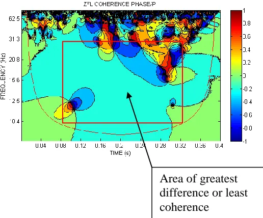
Figure 12: Example of Coherence Phase
Generally speaking, the area of greatest difference that can be utilized occurs
between the times of 0.08 and 0.32 seconds and 10 to 30 Hertz as shown by the red box. This is the area that will be used in the slicing method shown in the following section.
Wavelet Slicing Analysis
With the boundaries set by statistics and area of greatest difference identified, the next step is to view individual frequency slices of the power spectrum of the wavelet transform.
When the time based signal is transformed using complex wavelets, a 128 x 500 matrix is generated which corresponds with the number of scales and time counts. From
this matrix, the row corresponding with the frequency of interest can be singled out and graphed as follows.
Figure 13: Example of a Z Force Wavelet Slice at 25 Hz
The differences observed in Figure 13 indicate the amplitude of the male subjects is higher than the female around the point of maximum reaction in the frequency range of 25 Hz.
AUDIO ANALYSIS
The use of audio analysis for this type of signal has not been documented therefore, there is not a baseline or standard of reference to build upon. The following section will define the process by which force plate signals are converted to a modified audio signal through conversion of a .csv file to an audio file then isolating and magnifying
frequencies of interest.
The reader will not be able to hear the differences but, graphs of the audio spectrums are included in examples and Appendix F for a visual comparison.
CSV Conversion
Prior to creating a sound file, steps were taken to combine and prepare the .csv files. To make play back process easier, the female and male signals were combined into one file. This enables the listener to listen to the female signal then the male signal without hesitation. As with the wavelet transforms, edge effects will cause problems with the audio files, therefore, zeros were added to the front of each signal and to the end of the male signal. The final modification was to taper the end of the signals to zero. This was done to fade out the signal and reduce the edge effects. The result of these preparations may be viewed in Figure 14.
Audio Transformation
Differences between genders in the raw converted audio signals were not easily identified as a result, Audicity® was used to modify them [32]. The following figures identify the modifications performed on a sample file and the resultant signals.
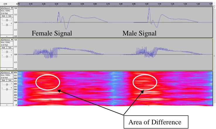
When viewing the output (Figure 14) from Audicity®, note that the top window is the original time based signal, the center is the modified time based signal, and the bottom window is the spectrum (similar to viewing the graph of a wavelet transform) of the modified time based signal. The time scale is noted along the top of the upper
window in the direction of the X axis. The Y axis in the upper and center windows is the magnitude of the signal and it represents a scaled frequency in the bottom window. The coloring in the spectrum correlates to the magnitude of the frequency at that point in time with red representing the highest magnitude and white representing the lowest magnitude.
Figure 14: Audio Signal Modifications
In this example, the pitch was increased by 700% and the tempo was decreased by 10%. Spectrum graphs for all of the audio signals may be found in Appendix F.
Female Signal Male Signal
CONCLUSIONS
The results of the analysis have shown that both wavelet and audio analyses can be used to further discern differences in force plate reactions between genders. The following sections will detail the findings and provide guidance for future studies.
Wavelet Transform Analysis
Using slices of wavelet transforms, differences between two signals at specific frequencies are easily viewed and can be referenced to specific events during the landing. In this case, the males and females were dominant in different areas which would support the hypothesis.
Audio Analysis
When the files are converted, modified, and played back the differences can be heard. The differences in these signals are at low frequencies. The differences are subtle however, with the right pitch shifting and amplification, they can be heard. Again, this would support the hypothesis.
Significance
The application for these methods goes beyond kinesiology however, the results may aid in understanding how the gender differences at low frequencies apply to injury rates.
maximum transmissibility of lower extremity muscles to be in the range of 5 to 20 Hz as shown in Figure 15 [8]. The study “Resonance Frequency in the Patellar Tendon” found those frequencies to be between 22 and 25 Hz dependant on the angle of the knee joint [9].
Transmissibility, also called the magnification factor, describes the factor of the input magnitude that is transferred to the mass being observed [33]. It is theorized that muscle damage occurs at these frequencies of maximum transmissibility, which generally coincides with the natural or resonant frequency of the system, as the power from the landing is amplified in the muscles. This range aligns with the regions of minimum coherence (value of 0) as shown on the coherence phase plots in Appendix D.
Figure 15: Mean Transmissibility of Lower Extremity Muscles
Future Studies
The methods used show that differences can be viewed using wavelet transforms and audio signals which would warrant further studies.
The considerations that need to be addressed prior to the study include the following: A method for building or gathering data for a base or reference signal for each
Several articles made reference to the potential effects of fatigue on these experiments therefore, protocol for limiting fatigue should be developed [3, 14, 34].
The method described here still relies on visual interpretation of graphs; quantification of a parameter(s) in the wavelet slices would enable a more uniform analysis. This quantification would also allow for statistical testing of the results.
Correlation to training methods and length of experience may impact the results of related studies.
REFERENCES
[1] J.M. Hootman, R. Dick, and J. Agel, “Epidemiology of collegiate injuries for 15 sports: Summary and recommendations for injury prevention initiatives,” Journal
of Athletic Training, vol. 42, (no. 2), pp. 311-319, Apr-Jun 2007.
[2] R.R. Lanese, R.H. Strauss, D.J. Leizman, and A.M. Rotondi, “Injury and Disability in Matched Mens and Womens Intercollegiate Sports,” American
Journal of Public Health, vol. 80, (no. 12), pp. 1459-1462, Dec 1990.
[3] E. Pappas, A. Sheikhzadeh, M. Hagins, and M. Nordin, “The effect of gender and fatigue on the biomechanics of bilateral landings from a jump: Peak values,”
Journal of Sports Science and Medicine, vol. 6, (no. 1), pp. 77-84, Mar 2007.
[4] K.A. Russell, R.M. Palmieri, S.M. Zinder, and C.D. Ingersoll, “Sex differences in valgus knee angle during a single-leg drop jump (vol 41, pg 166, 2006),” Journal
of Athletic Training, vol. 41, (no. 3), pp. 347-347, Jul-Sep 2006.
[5] P.S. Addison, The illustrated wavelet transform handbook, Bristol: Institute of Physics Publishing, 2002.
[6] C. Torrence and G.P. Compo, “A practical guide to wavelet analysis,” Bulletin of
the American Meteorological Society, vol. 79, (no. 1), pp. 61-78, Jan 1998.
[7] A. Grinsted, J.C. Moore, and S. Jevrejeva, “Application of the cross wavelet transform and wavelet coherence to geophysical time series,” Nonlinear
Processes in Geophysics, vol. 11, (no. 5-6), pp. 561-566, 2004.
[8] K.A. Boyer and B.M. Nigg, “Changes in muscle activity in response to different impact forces affect soft tissue compartment mechanical properties,” Journal of
Biomechanical Engineering-Transactions of the Asme, vol. 129, (no. 4), pp.
594-602, Aug 2007.
[10] R.P. Pfeiffer, M. Sabick, D. Clark, S. Kuhlman, K.G. Shea, K. Kipp, and K. Kipp, “Effect of Gender on Lower Extremity Muscle Activation in Children Performing A Single-Leg Unanticipated Landing Task,” Department of Mechanical and Biomedical Engineering, Boise State University, 2008.
[11] S.L. Grandstrand, R.P. Pfeiffer, M.B. Sabick, M. DeBeliso, and K.G. Shea, “The effects of a commercially available warm-up program on landing mechanics in female youth soccer players,” Journal of Strength and Conditioning Research, vol. 20, (no. 2), pp. 331-335, May 2006.
[12] M.T.G. Pain and J.H. Challis, “The influence of soft tissue movement on ground reaction forces, joint torques and joint reaction forces in drop landings,” Journal
of Biomechanics, vol. 39, (no. 1), pp. 119-124, 2006.
[13] A. Benjaminse, A. Habu, T.C. Sell, J.P. Abt, F.H. Fu, J.B. Myers, and S.M. Lephart, “Fatigue alters lower extremity kinematics during a single-leg stop-jump task,” Knee Surgery Sports Traumatology Arthroscopy, vol. 16, (no. 4), pp. 400-407, Apr 2008.
[14] E. Coventry, K.M. O'Connor, B.A. Hart, J.E. Earl, and K.T. Ebersole, “The effect of lower extremity fatigue on shock attenuation during single-leg landing,”
Clinical Biomechanics, vol. 21, (no. 10), pp. 1090-1097, Dec 2006.
[15] T.W. Kernozek, M.R. Torry, H. Van Hoof, H. Cowley, and S. Tanner, “Gender differences in frontal and sagittal plane biomechanics during drop landings,”
Medicine and Science in Sports and Exercise, vol. 37, (no. 6), pp. 1003-1012, Jun
2005.
[16] T.S. Gross and R.C. Nelson, “The Shock Attenuation Role of the Ankle During Landing From a Vertical Jump,” Medicine and Science in Sports and Exercise, vol. 20, (no. 5), pp. 506-514, Oct 1988.
[17] C.R. Carcia and R.L. Martin, “The influence of gender on gluteus medius activity during a drop jump,” Physical Therapy in Sport, vol. 8, (no. 4), pp. 169-176, Nov 2007.
[18] T. Mathworks, “MATLAB R2007a, Version 7.4.0.287,” 2007.
[19] Z. Ge, “Significance tests for the wavelet power and the wavelet power spectrum,” Annales Geophysicae, vol. 25, (no. 11), pp. 2259-2269, 2007. [20] H. Bachcivan, N. Zhang, M.A. Mirski, and D. Sherman, “Cross-Correlation
Analysis of Epileptiform Propagation Using Wavelets,” Department of
[21] G.R.J. Cooper and D.R. Cowan, “Comparing time series using wavelet-based semblance analysis,” Computers & Geosciences, vol. 34, (no. 2), pp. 95-102, Feb 2008.
[22] L. Kren, “Vibes Scope Machine Health,” Machine Design Magazine, 2007. [23] M. Stalbom, D.J. Holm, J.B. Cronin, and J.W.L. Keogh, “Reliability of
kinematics and kinetics associated with Horizontal Single leg drop jump
assessment. A brief report,” Journal of Sports Science and Medicine, vol. 6, (no. 2), pp. 261-264, Jun 2007.
[24] J. Abian, L.M. Alegre, A.J. Lara, J.A. Rubio, and X. Aguado, “Landing
differences between men and women in a maximal vertical jump aptitude test,”
Journal of Sports Medicine and Physical Fitness, vol. 48, (no. 3), pp. 305-310,
Sep 2008.
[25] N. Cortes, J. Onate, J. Abrantes, L. Gagen, E. Dowling, and B. Van Lunen, “Effects of gender and foot-landing techniques on lower extremity kinematics during drop-jump landings,” Journal of Applied Biomechanics, vol. 23, (no. 4), pp. 289-299, Nov 2007.
[26] T.M. Stephens, B.R. Lawson, D.E. DeVoe, and R.F. Reiser, “Gender and bilateral differences in single-leg countermovement jump performance with comparison to a double-leg jump,” Journal of Applied Biomechanics, vol. 23, (no. 3), pp. 190-202, Aug 2007.
[27] L. Scheef, H. Boecker, M. Daamen, U. Fehse, M.W. Landsberg, D.O. Granath, H. Mechling, and A.O. Effenberg, “Multimodal motion processing in area V5/MT: Evidence from an artificial class of audio-visual events,” Brain Research, vol. 1252, pp. 94-104, Feb 2009.
[28] K.I. AG, “Multicomponent Force Plate Type 9281C for Dynamic Applications in Biomechanics, Fz –10 ... 20 kN,” 2007.
[29] K.I. AG, “BioWare Version 4.0,” 2008.
[30] N.I. Corporation, “Labview Version 8.0,” 2005.
[31] R.H. McCuen, Statistical Methods for Engineers, Englewood Cliffs: Prentice Hall, Inc., 1985.
[32] A.D. Team, “Audacity® 1.3.7 (Unicode),” 2009.
APPENDIX A
APPENDIX B
APPENDIX C
Figure C.1: X Force Left Leg Wavelet Transforms
Figure C.3: Y Force Left Leg Wavelet Transforms
Figure C.5: Z Force Left Leg Transforms
Figure C.7: Z Moment Left Leg Wavelet Transforms
APPENDIX D
Figure D.1: X Force Left/Right Leg Coherence Phase
Figure D.2: Y Force Left/Right Leg Coherence Phase
APPENDIX E
Figure E.1: X Force Left Leg Slices
Figure E.3: Y Force Left Leg Slices
Figure E.5: Z Force Left Leg Slices
Figure E.7: Z Moment Left Leg Slices
APPENDIX F
Figure F.1: X Force Left Leg Audio Signals
Modifications: Pitch: +700%, Tempo: -10%
Figure F.2: X Force Right Leg Audio Signals
Figure F.3: Y Force Left Leg Audio Signals
Modifications: First Strike Removed, Pitch: +700%, Tempo: -10%
Figure F.4: Y Force Right Leg Audio Signals
Figure F.5: Z Force Left Leg Audio Signals
Modifications: Pitch: +600%, Tempo: -20%
Figure F.6: Z Force Right Leg Audio Signals
Figure F.7: Z Moment Left Leg Audio Signals
Modifications: Pitch: +700%, Tempo: -20%
Figure F.8: Z Moment Right Leg Audio Signals
APPENDIX G
TABLE OF CONTENTS
Averaging Program ... 64
Fourier Transform Program ... 65
Wavelet Transform and Statistics Program ... 66
Coherence Plot Program ... 68
Wavelet Transform and Slicing Program ... 69
Averaging Program
% **************************************************************** % *** Program written by Wes Orme
% *** Boise State University
% *** Program will average individual trials and output averaged signal and graph % ****************************************************************
t1=500;
t=1:t1; t2=transpose(.0008:.0008:.4);
fileaxis=input('Input the axis being evaluated (i.e. X,Y,Z): ','s');%Input the base name of the file fm=input('Enter 1 for Force evaluation only or 2 for both Force and Moment: ');
a=0; while a<fm; b=0; a=a+1; if a<1.1 filefm='F'; else filefm='M'; end while b<2; x=0; b=b+1; if b<1.1 fileleg='L'; else fileleg='R'; end
%Average input signals while x<2; x=x+1; z=0; if x<1.1 gen='F';qty=19; else gen='M';qty=16;y1=y2; end orsig=zeros(t1,1);
while z<qty; %subject number loop z=z+1; y=0; subnum=num2str(z); while y<10; %trial number loop y=y+1; trialnum=num2str(y);
fname=strcat('C:\',gen,filefm,fileaxis,'\',gen,subnum,fileleg,trialnum,'.csv'); orsig=orsig+csvread(fname);
end %trial number loop end %subject number loop m=z*10;
y2=transpose(orsig./(m)); z=0;
end
plot(t2,y1,'red'); hold all; plot(t2,y2,'green'); hold off; legend('FEMALE','MALE')
Fourier Transform Program
% *********************************************************************** % Program written by Joe Guarino and Wes Orme
% Boise State University
% Program will compute and display the Fourier Transform for the averaged time based signals % ************************************************************************ %Set constants t1=500; t=1:t1; a=0;
%Input the axis for which the analysis is to be done
fileaxis=input('Input the axis being evaluated (X,Y,or Z): ','s'); fm=input('If only the force is to be evaluated, enter 1, else enter 2: ');
while a<fm; %Loop # for forces and moments b=0; a=a+1;
if a<1.1
filefm='F'; tfm=' FORCE'; else
filefm='M'; tfm=' MOMENT'; end
while b<2; %leg loop x=0; b=b+1; if b<1.1
fileleg='L'; tleg=' LEFT'; else
fileleg='R'; tleg=' RIGHT'; end
filename = strcat('F',fileaxis,filefm,fileleg,'AVEFILE.csv'); y1 =csvread(filename);
filename = strcat('M',fileaxis,filefm,fileleg,'AVEFILE.csv'); y2 =csvread(filename);
%Compute constants needed for Fourier Transform maxdata=max(y1);
N = length(y1); NL = N/2; FS=1250;
%Calculate and display Fourier Transform of data NFFT=2^nextpow2(N);
Yf=fft(y1,NFFT)/N;
ff = FS/2*linspace(0,1,NFFT/2);
plot(ff,2*abs(Yf(1:NFFT/2)),'red'); hold all; Yf=fft(y2,NFFT)/N;
ff = FS/2*linspace(0,1,NFFT/2);
plot(ff,2*abs(Yf(1:NFFT/2)),'green'); hold off; legend('FEMALE','MALE')
Wavelet Transform and Statistics Program
% ******************************************************************* % Program written by Wes Orme, Wayne Fischer, and Joe Guarino.
% Boise State University
% Program will do the following for the averaged files:
% Perform a Complex Morlet Wavelet transform, with central frequency and bandwidth of 1 Hz % Calculate the Cone of Influence and Significance Contours (assuming white noise). % Plot the wavelet transform power, cone of influence, and significance contours. %*********************************************************************
%---INPUT MODULE--- fileaxis=input('Input axis to be analyzed (X,Y,or Z): ','s'); filefm=input('Input force or moment to be analyzed (F or M): ','s'); fileleg=input('Input leg to be analyzed (L or R): ','s');
filename = strcat('F',fileaxis,filefm,fileleg,'AVEFILE.csv'); datafile=csvread(filename);
%---CONSTANTS--- dt =.0008;% Time in seconds between data points siglev=.95; %Desired significance level, from 0.99 to 0.80 %---
maxdata=max(datafile); N = length(datafile); NL = N/2; FS=1/dt;
%---FEMALE WAVELET TRANSFORM AND PLOT--- ww1 = cwt(datafile,1:1:128,'cmor1-1');
wwa=(abs(ww1)).^2; %create power spectrum from coefficient matrix upswwa = flipud(wwa);
subplot(1,2,1)
contourf(upswwa),colormap(jet); xlim([0 500]); set(gca,'YTickLabel',[10.4;12.5;15.6;20.8;31.3;62.5]); ax=get(gca,'XTicklabel');
Bnum=str2num(ax); BF=dt*Bnum;
set(gca,'XTicklabel',BF);
ylabel('Frequency (Hz)'); xlabel('Time (s)'); colorbar('location','eastoutside'); title('FEMALE WAVELET TRANSFORM');
hold on
% Calculate and plot cone of influence ci=0;
for t = 1:NL
ci(t,1)=(1.373/(t*dt)); end
N2L=NL+1; for t = N2L:N
ci(t,1)=((1.373/((N-t)*dt))); end
plot(ci,'red');
% Calculate and plot Significance contours sigma = std(datafile);
% Zero Out significance matrix for nr = 1:128
for nc = 1:N sigmat(nr,nc)=0; end
end
% Create vector of chi-squared values
chive(1)= 9.2103;chive(2)=7.8240;chive(3)=7.0131;chive(4)=6.4377;chive(5)=5.9914; chive(6)=5.6268;chive(7)=5.3185;chive(8)=5.0514;chive(9)=4.8158;chive(10)=4.6051; chive(11)=4.4145;chive(12)=4.2405;chive(13)=4.0804;chive(14)=3.9322;chive(15)=3.7942; chive(16)=3.6651;chive(17)=3.5439;chive(18)=3.4295;chive(19)=3.3214;chive(20)=3.2188; for i = 1:128
alpha = .01*k; sigcheck=(sigma^2)*dt*chive(k)/2; if upswwa(i,j)>sigcheck sigmat(i,j)=1-alpha; end end end end hold on
[C,h] = contour(sigmat,siglev,'k'); clabel(C,h,'LabelSpacing',288,'Rotation',0); hold off
%---MALE WAVELET TRANSFORM AND PLOT--- filename = strcat('M',fileaxis,filefm,fileleg,'AVEFILE.csv');
datafile=csvread(filename);
ww1 = cwt(datafile,1:1:128,'cmor1-1');
wwa=(abs(ww1)).^2; %create power spectrum from coefficient matrix upswwa = flipud(wwa);
subplot(1,2,2)
contourf(upswwa),colormap(jet); xlim([0 500]); set(gca,'XTicklabel',BF);
set(gca,'YTickLabel',[10.4;12.5;15.6;20.8;31.3;62.5]);
ylabel('Frequency (Hz)'); xlabel('Time (s)'); colorbar('location','eastoutside'); title('MALE WAVELET TRANSFORM');
hold on
% Calculate and plot cone of influence plot(ci,'red')
% Calculate and plot Significance contours sigma = std(datafile);
% Zero Out significance matrix for nr = 1:128
for nc = 1:N sigmat(nr,nc)=0; end
end
% Create vector of chi-squared values
chive(1)= 9.2103;chive(2)=7.8240;chive(3)=7.0131;chive(4)=6.4377;chive(5)=5.9914; chive(6)=5.6268;chive(7)=5.3185;chive(8)=5.0514;chive(9)=4.8158;chive(10)=4.6051; chive(11)=4.4145;chive(12)=4.2405;chive(13)=4.0804;chive(14)=3.9322;chive(15)=3.7942; chive(16)=3.6651;chive(17)=3.5439;chive(18)=3.4295;chive(19)=3.3214;chive(20)=3.2188; for i = 1:128
for j = 1:N for k =20:-1.0:1.0 alpha = .01*k;
sigcheck=(sigma^2)*dt*chive(k)/2; if upswwa(i,j)>sigcheck sigmat(i,j)=1-alpha; end end end end hold on
[C,h] = contour(sigmat,siglev,'k'); clabel(C,h,'LabelSpacing',288,'Rotation',0); hold off
Coherence Plot Program
%****************************************************************** % Written by Wes Orme
% Boise State University
% Coherence Plot is generated for the wavelet transforms of the averaged files %******************************************************************
%---INPUT MODULE--- fileaxis=input('Input axis to be analyzed (X,Y,Z): ','s'); filefm=input('Input force or moment to be analyzed (F,M): ','s'); fileleg=input('Input leg to be analyzed (L,R): ','s');
filename = strcat('F',fileaxis,filefm,fileleg,'AVEFILE.csv'); y1 =csvread(filename);
filename = strcat('M',fileaxis,filefm,fileleg,'AVEFILE.csv'); y2 =csvread(filename);
t1=500; t=1:t1; nscales=128;
% Perform the wavelet transforms and compute the semblance c1=cwt(y1,1:nscales,'cmor1-1');
c2=cwt(y2,1:nscales,'cmor1-1'); % Compute the CWT's ctc=c1.*conj(c2); % Cross wavelet transform amplitude spt=atan2(imag(ctc),real(ctc)); % Cross wavelet phase cp=spt/pi;
cp=flipud(cp); %Invert cp matrix
%Plot coherence phase and save figure
titlename=strcat(fileaxis,filefm,fileleg,' COHERENCE PHASE/PI'); contourf(cp)
hold on
% Calculate and plot cone of influence ci=0;
for t = 1:NL
ci(t,1)=(1.373/(t*dt)); end
N2L=NL+1; for t = N2L:N
ci(t,1)=((1.373/((N-t)*dt))); end
plot(ci,'red');
% Calculate and plot Significance contours sigma = std(datafile);
hold off set(gca,'YTickLabel',[10.4;12.5;15.6;20.8;31.3;62.5]); ax=get(gca,'XTicklabel'); Bnum=str2num(ax); BF=dt*Bnum; set(gca,'XTicklabel',BF); title(titlename); colorbar('location','eastoutside')
Wavelet Transform and Slicing Program
% ******************************************************************** % Program written by Wes Orme
% Boise State University
% Program will extract lines from wavelet transform power matrices and generate plots % *********************************************************************
%Set constants
t1=500; t=1:t1; x=0; dt=0.0008;
%Input Parameters for files to be analyzed
fileaxis=input('Input the axis being evaluated (X,Y, or Z): ','s'); filefm=input('Is the force or moment being evaluated (F or M): ','s'); fileleg=input('Is the left or right leg being evaluated (L or R): ','s');
% Read in files
filename = strcat('F',fileaxis,filefm,fileleg,'AVEFILE.csv'); y1=csvread(filename);
filename = strcat('M',fileaxis,filefm,fileleg,'AVEFILE.csv'); y2=csvread(filename);
% Perform the wavelet transforms c1=cwt(y1,1:128,'cmor1-1'); c2=cwt(y2,1:128,'cmor1-1');
%Parse sub matrices
st=100; se=400; %set starting and ending time points cf110=abs(c1(18,st:se)).^2; cm110=abs(c2(18,st:se)).^2; cf100=abs(c1(28,st:se)).^2; cm100=abs(c2(28,st:se)).^2; cf90=abs(c1(38,st:se)).^2; cm90=abs(c2(38,st:se)).^2; cf80=abs(c1(48,st:se)).^2; cm80=abs(c2(48,st:se)).^2; cf70=abs(c1(58,st:se)).^2; cm70=abs(c2(58,st:se)).^2; cf60=abs(c1(68,st:se)).^2; cm60=abs(c2(68,st:se)).^2; cf50=abs(c1(78,st:se)).^2; cm50=abs(c2(78,st:se)).^2; cf40=abs(c1(88,st:se)).^2; cm40=abs(c2(88,st:se)).^2;
%Generate plot and save
subplot(4,2,1);plot(cf110', 'r'); hold all; plot(cm110', 'g'); hold off;
tname=strcat(fileaxis,filefm,fileleg,' 11.36 Hz WAVELET SLICE'); title(tname); ylabel('MAGNITUDE'); legend('FEMALE','MALE');
ax=get(gca,'XTicklabel'); Bnum=str2num(ax); BF=dt*(Bnum+st); set(gca,'XTicklabel',BF);
subplot(4,2,2);plot(cf100', 'r'); hold all; plot(cm100', 'g'); hold off;
tname=strcat(fileaxis,filefm,fileleg,' 12.50 Hz WAVELET SLICE'); title(tname); ylabel('MAGNITUDE'); legend('FEMALE','MALE');
set(gca,'XTicklabel',BF);
subplot(4,2,3);plot(cf90', 'r'); hold all; plot(cm90', 'g'); hold off;
tname=strcat(fileaxis,filefm,fileleg,' 13.89 Hz WAVELET SLICE'); title(tname); ylabel('MAGNITUDE'); legend('FEMALE','MALE');
set(gca,'XTicklabel',BF);
subplot(4,2,4);plot(cf80', 'r'); hold all; plot(cm80', 'g'); hold off;
tname=strcat(fileaxis,filefm,fileleg,' 15.63 Hz WAVELET SLICE'); title(tname); ylabel('MAGNITUDE'); legend('FEMALE','MALE');
set(gca,'XTicklabel',BF);
subplot(4,2,5);plot(cf70', 'r'); hold all; plot(cm70', 'g'); hold off;
tname=strcat(fileaxis,filefm,fileleg,' 17.86 Hz WAVELET SLICE'); title(tname); ylabel('MAGNITUDE'); legend('FEMALE','MALE');
set(gca,'XTicklabel',BF);
subplot(4,2,6);plot(cf60', 'r'); hold all; plot(cm60', 'g'); hold off;
tname=strcat(fileaxis,filefm,fileleg,' 20.83 Hz WAVELET SLICE'); title(tname); ylabel('MAGNITUDE'); legend('FEMALE','MALE');
set(gca,'XTicklabel',BF);
subplot(4,2,7);plot(cf50', 'r'); hold all; plot(cm50', 'g'); hold off;
set(gca,'XTicklabel',BF);
subplot(4,2,8);plot(cf40', 'r'); hold all; plot(cm40', 'g'); hold off;
tname=strcat(fileaxis,filefm,fileleg,' 31.25 Hz WAVELET SLICE'); title(tname); xlabel('TIME (s)'); ylabel('MAGNITUDE'); legend('FEMALE','MALE'); set(gca,'XTicklabel',BF);
%Save plot
titlename=strcat(fileaxis,filefm,fileleg,'_SLICEABS'); hgsave(titlename);
Converting CSV to WAV Files
% Program written by Wes Orme % Boise State University
% This program normalizes a csv file so the values fall between +/-1 % Adds slope to the end of each signal back to 0
% Combines male and female signals with 250 counts between them
% Input parameters
fileaxis=input('Input axis to be analyzed (X,Y,or Z): ','s'); filefm=input('Input force or moment to be analyzed (F or M): ','s'); fileleg=input('Input leg to be analyzed (L or R): ','s');
Fs=1250; %Data sample rate
% Read in female file
filename = strcat('F',fileaxis,filefm,fileleg,'AVEFILE.csv'); ffile=csvread(filename);
% Read in male file
filename = strcat('M',fileaxis,filefm,fileleg,'AVEFILE.csv'); mfile=csvread(filename);
%Build slope arrays
fslope=[ffile(1,500):-ffile(1,500)/125:0]; mslope=[mfile(1,500):-mfile(1,500)/125:0];
% Combine files
fcom=[ zeros(1,250),ffile,fslope,zeros(1,250),mfile,mslope,zeros(1,250)];
% Normalize file
fcomn=fcom./(max(abs(fcom)));
% Write wav files