VOLUME 37, ARTICLE 56, PAGES 1793
,
1824
PUBLISHED 8 DECEMBER 2017
http://www.demographic-research.org/Volumes/Vol37/56/ DOI: 10.4054/DemRes.2017.37.56
Research Article
The wage penalty for motherhood:
Evidence on discrimination from panel data and
a survey experiment for Switzerland
Daniel Oesch
Oliver Lipps
Patrick McDonald
© 2017 Daniel Oesch, Oliver Lipps & Patrick McDonald.
This open-access work is published under the terms of the Creative Commons Attribution 3.0 Germany (CC BY 3.0 DE), which permits use, reproduction, and distribution in any medium, provided the original author(s) and source are given credit.
1 Introduction 1794
2 The theoretical links between motherhood and wages 1796 2.1 A motherhood wage gap driven by productivity 1796 2.2 A motherhood wage gap driven by discrimination 1797
3 Country selection, data, and methods 1798
3.1 Country differences in the wage penalty 1798
3.2 Longitudinal surveys 1799
3.2.1 Data 1799
3.2.2 Measures 1800
3.2.3 Model specification 1801
3.3 Factorial survey experiment 1801
3.3.1 The logic behind factorial survey experiments 1801
3.3.2 The construction of our experiment 1802
3.3.3 Estimation method 1803
4 Panel data evidence of the motherhood wage gap 1804
5 Experimental evidence for the motherhood wage gap 1806
6 Conclusion 1811
7 Acknowledgements 1812
References 1814
The wage penalty for motherhood:
Evidence on discrimination from panel data and a survey
experiment for Switzerland
Daniel Oesch1 Oliver Lipps2
Patrick McDonald3
Abstract
BACKGROUND
Survey-based research finds a sizeable unexplained wage gap between mothers and nonmothers in affluent countries. The source of this wage gap is unclear: It can stem either from the unobserved effects of motherhood on productivity or from employer discrimination against mothers.
OBJECTIVE
This paper opens the black box of the motherhood wage gap by directly measuring discrimination in Switzerland based on two complementary methods.
METHODS
We first use two longitudinal population surveys to establish the size of the wage residual for motherhood. We then run a factorial survey experiment among HR managers (N=714) whom we asked to assign a starting wage to the résumés of fictitious job candidates.
RESULTS
The population surveys show an unexplained wage penalty per child of 4% to 8%. The factorial survey experiment shows that recruiters assign wages to mothers that are 2% to 3% below those of nonmothers. The wage penalty is larger for younger mothers, 6% for ages 40 and less, but disappears for older mothers or mothers in a blue-collar occupation.
1 Life Course and Inequality Research Centre (LINES), Université de Lausanne, Switzerland.
E-Mail:[email protected].
CONCLUSION
The motherhood wage gap found in panel studies cannot be reduced to unobserved dimensions of work productivity. The experimental evidence shows that recruiters discriminate against mothers.
CONTRIBUTION
Our paper’s novelty is to uncover wage discrimination against mothers by combining two different methods. Our national panel surveys mirror the supply side of the labor market and provide us with strong external validity. The factorial survey experiment on recruiters informs on the demand side of the labor market and shows a causal effect.
1. Introduction
Mothers tend to earn lower wages than nonmothers across the Western World. While differences in work experience and job characteristics go some way in accounting for this gap, most studies find a nontrivial unexplained wage residual. In Britain, Germany, and the United States, this residual varies between a low of 3%‒5% and a high of 8%‒ 10% per child and suggests that mothers incur an earnings penalty (e.g., Budig and England 2001; Gangl and Ziefle 2009; Glauber 2007; Killewald and Gough 2013; Harkness 2016).
The unexplained wage residual for motherhood may arise from two sources: the unobserved effects of motherhood on work productivity or employer discrimination against mothers. The challenge faced by the literature is to empirically disentangle the influence of these two sources (Mu and Xie 2016). Although surveys ask detailed questions about training, tenure, and occupation, it is impossible to measure all dimensions of work productivity. Therefore, if the goal is to open the black box of the motherhood wage residual it is necessary to resort to experimental methods that tap directly into discrimination (Correll, Benard, and Paik 2007: 1332).
However, while experiments provide high internal validity and allow researchers to draw causal conclusions, their external validity – and hence the degree to which the results can be generalized to other contexts – is often limited. In the context of the motherhood wage penalty, it is doubtful whether the wage recommendations of undergraduate students in an experimental study accurately reflect the actual wage-setting behavior of employers. Consequently, the two analytical methods – population surveys and experiments – should be combined within the same study to increase the robustness of findings.
representative longitudinal surveys and fixed-effects regressions to examine whether having children is associated with lower wages for working mothers. This allows us to establish the size of the unexplained wage residual for motherhood. We then test wage discrimination directly by carrying out a factorial survey experiment, a method also known as a vignette study. We show the résumés (vignettes) of fictional job candidates to 714 HR managers and ask them to indicate the wage that seems adequate for these candidates. By randomly varying a set of dimensions for each vignette (such as education, age, nationality, children), we are able to identify if – and how – the presence of children affects the wages that recruiters assign to candidates.
Our study uses data from Switzerland, a country that shares many labor market features with Germany, notably a large vocational education system, a tight link between education and employment, and wage bargaining at the industry level. However, Switzerland offers much less public support for maternal employment and, in terms of family policy, is more closely aligned to Britain or the United States. To the extent that comparative research has found systematic differences between these countries in the motherhood wage gap (Gangl and Ziefle 2009; Gash 2009), adding evidence on Switzerland helps us to better understand how this gap varies across institutional settings.
Our study is the first to combine the analysis of longitudinal surveys – the Swiss Household Panel and the Swiss Labor Force Survey – with a factorial survey experiment. The use of national population surveys provides us with insight into the supply side of the labor market – workers and their wages – and gives us strong external validity. The factorial survey experiment on recruiters, in turn, informs us of the demand side of the labor market – employers and their ratings – and helps us to unravel causal effects. Unlike earlier experimental studies on the topic, our vignette study does not rely on undergraduate students (Correll, Benard, and Paik 2007) or the general employed population (Denny 2016), but on active recruiters, and thus on individuals who, unlike students or workers, actually wield influence over wage-setting.
2. The theoretical links between motherhood and wages
2.1 A motherhood wage gap driven by productivity
Motherhood may hamper the evolution of wages because having children often interferes with mothers’ labor market attachment and thus reduces their productivity at work. On the one hand, children may lead to career interruptions and thus slow down mothers’ accumulation of human capital. On the other hand, raising children takes time and effort and may leave mothers with less energy for paid work.
According to the first explanation, the birth of children increases the likelihood that women interrupt their careers and thus accumulate less tenure and work experience than they would have without children. Survey research has identified mothers’ reduced work experience as the key determinant of the motherhood wage gap (Gangl and Ziefle 2009). In the United States the sharp increase in wages for extended work hours – and mothers’ lower propensity to take on such jobs – has further contributed to the wage penalty associated with children (Weeden, Cha, and Bucca 2016). More generally, when returning to employment, mothers often take on part-time jobs. This more tenuous attachment to the labor market decreases the incentive for mothers – and their employers – to invest in training and further education (Polavieja 2012). As a result, motherhood may slow down the growth in job-specific skills and lead to flatter career trajectories.
An alternative explanation also expects motherhood to decrease productivity at work. However, the central mechanism is not children’s effect on human capital, but on time and energy. The idea is that raising children takes effort and may thus interfere with the demands of paid work. To the extent that mothers carry the brunt of childcare – such as picking children up from school, caring for them when sick, attending their activities – they may have less energy to bring to the labor market and be less productive workers (Budig and England 2001: 206; Gangl and Ziefle 2009: 342).
This argument is taken a step further in the theory of compensating differentials. In the traditional household division of labor, mothers are expected to trade wages for family-friendly employment that is compatible with childcare duties (Becker 1973). Mothers may thus avoid jobs that pay well but make great demands in terms of constant availability, nonstandard hours, overtime work, or long travel. Once they have children, mothers may therefore switch to jobs with predictable work schedules and hence forgo well-paying jobs for part-time jobs in the public sector that allow them to take time off for family duties.
on studies with this design, there seems to be a gross wage penalty for the United States of 5% to 10% per child (Budig and England 2001: 219; Killewald and Gough 2013: 488). When controlling for work experience, seniority, and shifts to family-friendly jobs, the motherhood wage gap in the United States decreases to about 3% per child (Budig and England 2001: 219; Glauber 2007: 955; Kahn, García-Manglano, and Bianchi 2014: 66). The jury is still out as to whether the motherhood penalty is larger among low-earning (Budig and Hodges 2010; Cooke 2014) or high-earning women (England et al. 2016).
In a panel study of American, British, and German mothers, once work experience is accounted for, the motherhood wage gap disappears in the United States and Britain, but remains at over 10% per child in Germany (Gangl and Ziefle 2009: 363). A study using the European Community Household Panel also finds a particularly large gap for Germany and, to a lesser extent, for Britain (Gash 2009). By contrast, there does not seem to be much of a wage penalty for mothers in Denmark, Finland (Gash 2009), or Norway (Petersen, Penner, and Høgsnes 2014).
2.2 A motherhood wage gap driven by discrimination
The finding of a sizeable wage gap associated with motherhood leaves us wondering whether this unexplained residual is due to unobserved differences in productivity or to employer discrimination.
Traditionally, sociologists have been critical of the idea that wages are solely determined by workers’ marginal productivity (e.g., Jacobs and Steinberg 1990: 460). The importance of the bargaining process for wage-setting suggests that noneconomic factors such as power resources, cultural beliefs, and social norms also affect workers’ earnings, leaving room for discrimination.
The notion of statistical discrimination assumes that one group of workers (e.g., women with small children) are less productive than another group (e.g., women without small children). Since measuring the productivity of each individual is costly and time-intensive, employers pay higher wages to workers from the more productive group (Correll, Benard, and Paik 2007: 1302). Some employers possibly use the presence of children to infer women’s unobserved productivity and create a wage penalty for mothers relative to nonmothers.
normative expectations on the good mother – to be constantly available for her children (Correll, Benard, and Paik 2007: 1306). The dominant social norm across much of the western world, notably in the German-speaking countries, considers that mothers’ primary role is to be at home with their children, whereas her paid job is of secondary importance. The opposite norm applies to fathers whose primary role is to play the breadwinner, not to be the caretaker at home (Krüger and Levy 2001). Fathers are therefore seen as needing a family wage to support wife and children, whereas mothers are regarded as secondary earners whose wages merely supplement total household income. Motherhood may thus be a status characteristic that yields lower expectations in terms of an adequate wage (Auspurg, Hinz, and Sauer 2017: 182).
An American study combining an experiment among students with an audit study among employers shows that childless women are rated significantly higher than mothers in terms of competence, work commitment, promotion prospects, and recommendations for hire when they have otherwise identical résumés (Correll, Benard, and Paik 2007). The participants in the experiment recommended a starting wage for mothers that was 7% lower than the wage offered to women without children. Likewise, the audit study showed that prospective employers called mothers back only half as often as childless women. In comparison, fathers were not disadvantaged at any stage of the hiring process (Correll, Benard, and Paik 2007: 1333).
While research shows discrimination against white mothers in the United States, the evidence of discrimination against African-American or Latino mothers is weaker. A vignette study among employed adults (Denny 2016) and a longitudinal survey study (Glauber 2007) find a wage penalty in the United States only for white mothers and not for mothers from minority groups. One explanation is that the dominant social norm of the ‘good mother’ who should be constantly available to her children only applies to white women. By contrast, as women of color “were incorporated into the United States largely to [serve] as labor”, their family life and status as mothers may be regarded as secondary to their status as workers (Denny 2016: 30).
3. Country selection, data, and methods
3.1 Country differences in the wage penalty
employment,Switzerland comes closer to the United States and Britain than Germany. Swiss legislation only provides for 14 weeks of paid maternity leave, and there is no statutory right to either parental leave for fathers or subsidized childcare. Institutional childcare is expensive and covers a minority of children below 4 years. Moreover, since a normal full-time job implies long weekly hours (an average of 41.7 hours) and short holidays (20 days per year), the great majority of mothers in Switzerland work part-time. Among mothers with at least one child below 6 years, 83% work part-time(OFS 2016).
The weakness of public support for reconciling family and work implies that mothers in Switzerland are, much like in the United States, “exposed to the unfettered operation of […] labor markets” (Gangl and Ziefle 2009: 347). Interestingly, comparative studies indicate a larger raw wage gap between mothers and nonmothers in Britain and the United States than in Germany. However, once differences in work experience and human capital are accounted for, the net wage gap is larger in Germany than in the two English-speaking countries (Gangl and Ziefle 2009; Gash 2009). Depending on whether the motherhood wage gap is driven by the institutions governing the labor market or by family policy, one would expect results for Switzerland to be more closely aligned to those of either Germany or the United Kingdom and United States.
3.2 Longitudinal surveys
3.2.1 Data
Survey data on wages and working hours are fraught with missing observations and measurement error. We therefore try to increase the robustness of our results by following the practice of “identical analysis of parallel data” and use two different data sets (Firebaugh 2008). The replication across two panel studies permits us to gauge the uncertainty in the results due to common errors in surveys linked to coverage, sampling, nonresponse, and measurement (Groves 2004).
For both datasets, we restrict our analytical sample to women aged 20 to 50 and to person-years when respondents were employed as wage earners. We only include respondents with wage observations in at least two waves. For the SHP 1999‒2015 this leaves us with 3,115 persons and 12,769 person-years, each respondent contributing, on average, 4.1 years of observation. For the SLFS 1991‒2009 this leaves us with a sample of 26,409 persons and 71,531 person-years, each respondent contributing 2.7 years of observation.
3.2.2 Measures
Our dependent variable is hourly wage, which we obtain by dividing monthly wages by working hours. In the SHP we use contractual working hours and supplement them, where missing, with usual working hours. In the SLFS we use reported working hours and, where missing, translate the percentage of employment into weekly hours (employment of 100% corresponding to 42 hours). In order to account for “overwork” (Weeden, Cha, and Bucca 2016) we cap weekly working hours only at 60 hours in both datasets. We control for inflation and use the natural logarithm of constant Swiss francs (for 2010 in the SHP, 2011 in the SLFS), excluding potential outliers by dropping the top and bottom 1% of the hourly wage distribution.
Our key independent variable is the number of children in the household, measured as a categorical variable: no child, one, two, three or more children. In the SHP we only include biological children. In the SLFS the child variable captures all children aged 15 or under who live in the household (before 1997 only biological children were recorded)
We use a set of controls for differences in work productivity: years of education (SHP) or detailed levels of education (SLFS), participation in job training, supervisory status, and, in the SHP, whether the respondent reports to be over-, under- or inadequately qualified for her job. Since there are no direct measures of work experience we construct our own measure in the SHP by calculating, for each person-year, the observed years in employment. In the SLFS we are forced to use job tenure as a proxy for experience.
We account for compensating differentials with control variables for the public sector, part-time employment, fixed-term contracts, firm size and, for the SHP, job change and employer change in the last year. We further control for the share of women in a given occupation4 (Murphy and Oesch 2016) and, in the SHP, for the prestige of an occupation (Treiman scale). In the SLFS we further control for occupation (ISCO
1-4 Using the Swiss Labor Force Survey, we calculate for each year the proportion of women in a job, based on
digit) and sector (NOGA). Finally, we enter variables for marriage and, in the SHP, the availability of external childcare and the weekly number of hours spent on housework (capped at 42 hours). All our models include dummies for the calendar year and age in years, which allows us to account for the age–earnings curve between the ages of 20 and 50.
3.2.3 Model specification
The effect of children on wages may be plagued by unobserved heterogeneity. If less productive women are more likely to have children, this leads to a spurious correlation between the number of children and wages. It has thus become standard to estimate the motherhood wage gap with fixed-effects panel models (e.g., Budig and England 2001; Gangl and Ziefle 2009; Kahn, García-Manglano, and Bianchi 2014). The fixed-effects estimator only takes account of the within-variance stemming from changes in women’s lives over time. This eliminates all observed and unobserved characteristics of the individual that do not vary over time, such as time-constant preferences and abilities which may affect both the decision to have children and the evolution of wages. By contrast, fixed effects do not eliminate unobserved time-varying characteristics that affect both a woman’s fertility decisions and her wage (Mu and Xie 2016).
The general equation for our person fixed-effects linear regressions is given as:
Yit = β0+ β1CHILDRENit+ β2CONTROLSit +i + εit (t=1, 2, …,T)
where Y is the logarithm of hourly wages for an individual i at time t. Our main predictor CHILDRENit is a time-varying categorical measure of the number of children of a womani at time t. CONTROLSit is a vector of control variables. We remove all time-invariant characteristics that differ between individuals by allowing i, a set of
unobserved time-constant variables, to correlate with all of our individual predictors. εit represents idiosyncratic error. Finally, we correct for the clustering of observations across waves by using panel-corrected standard errors.
3.3 Factorial survey experiment
3.3.1 The logic behind factorial survey experiments
decades (Rossi and Nock 1982), but were only recently taken up in economic sociology to study the preferences of employers (e.g., Di Stasio 2014; Liechti et al. 2017).
Factorial surveys simulate the hiring process by presenting the résumés of fictitious job candidates to respondents and asking them for ratings. They have two advantages over conventional surveys. First, they are less subject to social desirability bias. Sensitive attributes (dimensions) such as age, gender, nationality, and motherhood status are randomly combined in the résumés (vignettes). These ever-changing combinations make it difficult for respondents to pick out and provide a politically correct answer to the one dimension which researchers are interested in. Auspurg et al. (2017) illustrate this point in a study of the gender wage gap.
Second, factorial surveys use an experimental set-up where the researcher fully controls the information shown to respondents. This eliminates a source of bias that is omnipresent in conventional surveys: unobserved characteristics (such as the abilities of a job candidate) that are collinear with the variable of interest (such as wages).
Note, however, that factorial surveys are experiments, and thus present hypothetical scenarios and only reflect stated intentions, not observable actions. Accordingly, the external validity of findings is open to discussion. This is particularly the case when survey experiments on recruitment are done with students (Correll, Benard, and Paik 2007) or random adults (Denny 2016), whose judgements may well differ from those of the specific group of recruiters.
3.3.2 The construction of our experiment
Our experiment addresses this last issue by surveying the members of a large human resources management association in Switzerland. In 2016 we sent a web-based questionnaire to 4,687 HR managers. We obtained responses from 714 individuals and thus a response rate of about 15%.5 Ninety-one percent of all respondents had been actively involved in at least one recruitment over the last 12 months, the median number of recruitments being ten. Our analytical sample only includes these active recruiters, 82% of whom claimed to have decisive influence over who gets hired for a job. Overall, our recruiters disproportionately came from large firms, the canton of Zurich, and the public sector.
We framed our experiment as a study into the hiring practices in different regions and sectors. It started with the description of a job vacancy in three occupations, followed by the presentation of fictitious résumés (see the vignette shown in Figure A-1 of the Appendix). Each respondent was asked to evaluate a random set of 12 résumés,
5 63% of the respondents were female and 37% male, with a mean age of 46 years. 70% of the respondents
four for each occupation. We selected three occupations – accountant, human resources assistant, and building maintenance worker (caretaker) – that cover a broad skills spectrum, are not clearly male- or female-dominated, and can be found in many firms across sectors. The order in which vignettes were presented was randomized.
For the résumé of each job candidate we asked recruiters to answer two questions: the likelihood that they would invite him or her to an interview on a scale from 0 to 10, and the monthly wage that seemed adequate for a given candidate, regardless of the likelihood of a job interview.
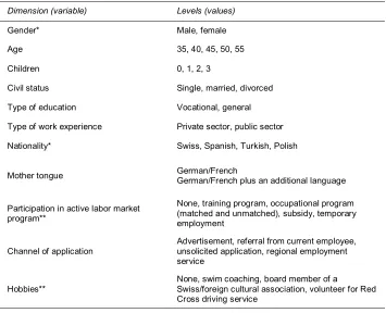
The profiles of our job candidates – the vignettes – are made up of 11 dimensions, including age, gender, nationality, civil status, type of education, work experience, and number of school-age children (see Table A-1 in the Appendix). Note that it is common in Switzerland to indicate the number of children in a CV.
From the combination of all possible vignettes (5,529,600 unique vignettes per occupation) we drew an orthogonal (d-efficient) sample of 720 vignettes per occupation (Auspurg and Hinz 2015).6 Thanks to randomization, vignette dimensions such as nationality, civil status, and motherhood are uncorrelated with each other (see Table A-2 in the Appendix for the correlation matrix).
Taking out nonresponses, using only active recruiters, and focusing on female job candidates aged 50 or younger, we are left with 385 recruiter responses that provide us with wage recommendations for 1,644 candidates. These 1,644 wage observations constitute our analytical sample.
3.3.3 Estimation method
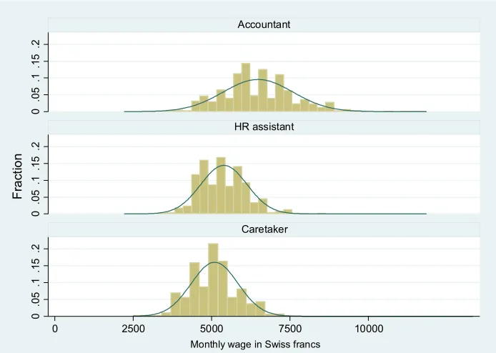
Our dependent variable is the natural logarithm of the monthly wage. Figure A-2 in the Appendix shows the distribution of monthly wages and suggests that the recruiters attributed plausible values to the different job candidates.
Our key independent variable is the number of school-age children, ranging from 0 to 3. Each quarter of our fictitious job candidates has values of 0, 1, 2, and 3 children, respectively. As job candidates applied for different occupations, occupation and the interaction between occupation and children are the two central control variables. In addition we control for civil status, nationality, type of education, and work experience. Note, however, that due to the experimental set-up, these control variables do not alter the results.
Our factorial survey produces data with a nested structure, as the same respondent rates up to 12 vignettes. Depending on a respondent’s own labor market experience, he
6 We implemented a D-efficient design that uses an algorithm to minimize intercorrelation between vignette
or she is prone to set a lower or higher baseline in terms of wages. Moreover, respondents are likely to attribute wages to successive vignettes by comparing them with the wage they attributed to the first vignette. These arguments plead for a respondent fixed-effects regression model that eliminates differences in respondents’ individual baselines. We thus only use the within-respondent variance; that is, the differences stemming from a respondent’s ratings of different vignettes. Our model’s equation is given as:
Yir = β0+ β1OCCir + β2CHILDir+ β2OCCir*CHILDir+ β3CONTROLSir +r + εir (r=1, 2, …R)
where Yir is the logarithm of monthly wages for a vignettei evaluated by a respondent r. OCCir is a control for occupation, CHILDir is a categorical measure of the number of children, OCCir*CHILDir is an interaction term, and CONTROLSir a vector of sociodemographic control variables of the fictitious job candidates. We remove all characteristics that differ between respondents by allowing r, a set of unobserved
variables, to correlate with all of our individual predictors. εir represents the idiosyncratic random error. We correct for the clustering of observations within respondents by using clustered standard errors.
4. Panel data evidence of the motherhood wage gap
Figure 1 reports the wage penalty associated with having children for women aged 20 to 50 for the two longitudinal population surveys, showing the percentage change in earnings for each child. Table A-3 in the Appendix shows the precise coefficients and standard errors. We first discuss the gross motherhood wage penalty – the raw gap in hourly wages without any other controls than age and calendar year – and then move on to the net wage penalty by controlling for differences in human capital and the work setting.
As expected, having children is associated with a relative decrease in women’s hourly wages. However, we find a much lower gross wage penalty for motherhood than studies on the United States. The first child has basically no influence in either dataset. The second child goes along with a decrease in wages of 2% (SLFS) to 4% (SHP). Estimations for the third child are less precise and vary between basically no penalty (SLFS) and 5% (SHP).
among mothers who remain in the labor force. As a result, the decrease in hourly wages is much smaller. However, the wage returns to hours diminish above 40 hours per week (Morgan and Arthur 2005). Therefore, dividing the wages of full-time employees (who are paid for 40 to 42 contractual hours) by reported working hours (e.g., 45 to 55 hours) may lead to an underestimation of their hourly earnings relative to part-time employees. This division bias problem understates the initial wages of those in full-time employment and overstates those of workers in part-time employment (Manning and Swaffield 2008: 993). This is crucial because motherhood in Switzerland often goes along with a transition from full-time to part-time employment, with reported working hours (notably those above 40 hours per week) falling more than earnings.
Therefore, we re-estimate the gross wage penalty by introducing an additional dummy variable for part-time employment which may capture over-reporting of hours among time employees (and diminishing wage returns to hours beyond the full-time schedule of 40 hours). When controlling for the transition to part-full-time employment the wage penalty for children becomes much larger. It amounts to 4% (first child), 5% (second child), and 3% (third child) in the SLFS and to 9% (first), 14% (second), and 15% (third child) in the SHP.
Figure 1: The reduction in hourly wages for motherhood in Switzerland
Note: SHP stands for the Swiss Household Panel, SLFS for Swiss Labor Force Survey. Results from fixed-effects linear regressions on (log) hourly wages for women aged 20 to 50 who are in the labor force. Strictly speaking, results are not percentages, but log points.
The model without controls includes age in years and calendar years, the model with all controls includes variables for part-time, human capital, type of job, and household arrangement. See Tables A-2 and A-3 for the complete models.
In a last model we account for differences in human capital and job characteristics and are thus able to decrease the wage penalty of motherhood by a third in the SHP. It falls to 6% for the first child and to 9% for the second and third child. In the SLFS, where we have no measures for job and employer change or the match of qualifications and housework, the full model only leads to a small decrease in the motherhood wage penalty, which remains at 3% to 4% per child.
These net wage penalties are upper-bound estimates. Our measure of work experience is far from perfect and may well overestimate mothers’ effective labor force experience, thereby leading to an overly large wage residual for motherhood. While we would have expected a larger decrease in the net wage penalty once we control for job characteristics, our result echoes the findings of Gash (2009: 580) who, based on the European Community Household Panel, reports an increase in the motherhood wage penalty for Denmark, France, Germany, and the United Kingdom once differences in human capital and the work setting are controlled for.
Overall, our two longitudinal surveys provide negative estimates for children’s effect on mothers’ hourly wages that range between a lower bound estimate of 2% to 4% and a higher bound of 6% to 9% per child, with possibly a smaller penalty for the first than for the second and third child. Since these coefficients may hide the unobserved effects that children have on women’s work productivity (and thus cannot be interpreted as solely reflecting wage discrimination against mothers), we turn to the factorial survey experiment, which tries to tap directly into discrimination.
5. Experimental evidence for the motherhood wage gap
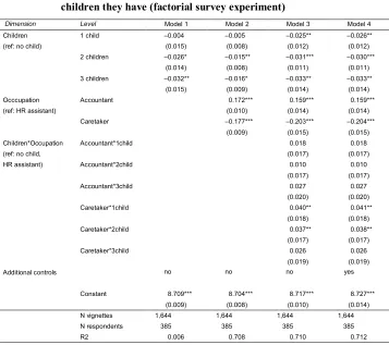
Table 1 shows how the presence of children affects the wages that recruiters deem adequate for female job candidates. In model 1 we simply regress the number of children on wages. While one child has no influence, recruiters assign wages to women with two or three children that are 3% lower than those deemed appropriate for women without children, all else being equal. Thus the unexplained wage residual also pops up in our factorial survey experiment.
This effect refers to the reference category of HR assistants. The positive interaction terms for building caretakers with children indicate that motherhood is deemed much less consequential for building caretakers than for HR assistants. If we add up the main effects for children with the interaction effects between children and occupation, we find that motherhood has no effect on the wage recommendations for caretakers. In the third occupation of accountants there is a wage penalty only for mothers with two children (2%).
Table 1: Wage recommendations for women depending on the number of children they have (factorial survey experiment)
Dimension Level Model 1 Model 2 Model 3 Model 4
Children 1 child ‒0.004 ‒0.005 ‒0.025** ‒0.026**
(ref: no child) (0.015) (0.008) (0.012) (0.012)
2 children ‒0.026* ‒0.015** ‒0.031*** ‒0.030***
(0.014) (0.008) (0.011) (0.011)
3 children ‒0.032** ‒0.016* ‒0.033** ‒0.033**
(0.015) (0.009) (0.014) (0.014)
Occcupation Accountant 0.172*** 0.159*** 0.159***
(ref: HR assistant) (0.010) (0.014) (0.014)
Caretaker ‒0.177*** ‒0.203*** ‒0.204***
(0.009) (0.015) (0.015)
Children*Occupation Accountant*1child 0.018 0.018
(ref: no child, (0.017) (0.017)
HR assistant) Accountant*2child 0.010 0.010
(0.017) (0.017)
Accountant*3child 0.027 0.027
(0.020) (0.020)
Caretaker*1child 0.040** 0.041**
(0.018) (0.018)
Caretaker*2child 0.037** 0.038**
(0.017) (0.017)
Caretaker*3child 0.026 0.026
(0.019) (0.019)
Additional controls no no no yes
Constant 8.709*** 8.704*** 8.717*** 8.727***
(0.009) (0.008) (0.010) (0.014)
N vignettes 1,644 1,644 1,644 1,644
N respondents 385 385 385 385
R2 0.006 0.708 0.710 0.712
Note: Respondent fixed-effects regressions on (log) wages for women aged 35 to 50. Clustered standard errors in parentheses. Additional controls in M4 include: civil status, nationality, type of education, type of work experience; the full model M4 is shown in Table A-5 in the Appendix.
As expected, given our experimental design, all the coefficients remain unchanged if we further control, in model 4, for civil status, nationality, type of education, and work experience (see Table A-5 in the Appendix for the full model).
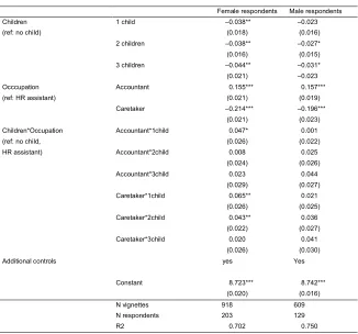
Our finding of wage discrimination against HR assistants with children holds true regardless of whether we select the answers of female or male recruiters. Female respondents are no less likely to discriminate against mothers than male respondents: on the contrary, female recruiters hand out even somewhat larger wage penalties to mothers than do male recruiters (see Table A-6 in the Appendix).
Our results raise the question of why recruiters would assign a wage penalty for children to HR assistants, but not to building caretakers and only partly to accountants? Our sample consists of HR managers who had been involved in hiring new staff over the past year. It is likely that HR managers’ expectations of job candidates destined to support them in their daily work – HR assistants – are clearer than of building caretakers or accountants, with whom they interact very loosely at best. Consequently, among the three occupations, their preferences regarding HR assistants should be the strongest and most clearly formulated.
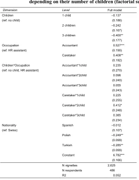
Table 2: The likelihood of getting invited to a job interview for women, depending on their number of children (factorial survey experiment)
Dimension Level Full model
Children 1 child ‒0.137
(ref: no child) (0.186)
2 children ‒0.242
(0.167)
3 children ‒0.400**
(0.177)
Occcupation Accountant 0.527***
(ref: HR assistant) (0.190)
Caretaker 0.408**
(0.192)
Children*Occupation Accountant*1child 0.235
(ref: no child, HR assistant) (0.270)
Accountant*2child 0.096 (0.240) Accountant*3child 0.055
(0.243)
Caretaker*1child 0.225
(0.255)
Caretaker*2child 0.412*
(0.248)
Caretaker*3child 0.385
(0.234)
Nationality Spanish ‒0.012
(ref: Swiss) (0.107)
Polish ‒0.249**
(0.099)
Turkish ‒0.285**
(0.099)
Constant 6.782***
(0.166)
N vignettes 2,625
N respondents 486
R2 0.052
Note: Respondent fixed-effects regressions on the likelihood to get invited to a job interview (on a scale 0-10) for women ages 35 to 50. Clustered standard errors in parentheses. Additional controls in M4 include: civil status, type of education, type of work experience.
*** p<0.01, ** p<0.05, * p<0.1
expects mothers to be at home child-rearing. The vignettes in our factorial survey simply indicated “school-age children,” leaving open an age range from 4 to 18. Each 20% of our fictitious female job candidates was attributed an age of 35, 40, 45, 50, or 55, respectively. We thus divide our pool of female job candidates into two age bands: 35‒40 and 45‒55.
Figure 2 shows how the effect of children on wages varies for these two age groups for the reference category of HR assistants. As expected, the wage loss incurred among mothers aged 35 to 40 is twice as large as that recorded for the extended sample of mothers shown above (aged 35 to 50). While it amounts to 2%‒3% in the extended sample, the wage penalty for a child doubles in the younger age group and reaches 6% for the first, second, and third child. Although these effects are estimated with large standard errors, they are all statistically significant at the 5% level and suggest that recruiters principally discriminate against younger mothers, possibly because they expect them to still be in the midst of their child-rearing years. By contrast, there is no wage penalty for older mothers aged 45 to 55.
Figure 2: The motherhood wage penalty for two different age groups of female job candidates (factorial survey experiment)
6. Conclusion
Survey-based research finds a sizeable wage gap between mothers and nonmothers in most affluent countries. However, we do not know whether this gap is due to (unobserved) differences in productivity or if it stems from discrimination against working mothers.
We have tried to open this black box and improve our understanding of the motherhood wage gap by combining two analytical methods. We first used two national panel studies to examine how women’s wages evolve before and after the birth of children. After controlling for human capital and job characteristics we found a net wage penalty of between 4% and 8% per child. This leaves us with wage residuals that are similar to those found for Germany (Gangl and Ziefle 2009; Gash 2009), but larger than those reported for the United States (Budig and England 2001; Glauber 2007).
We further probed into this unexplained wage residual by doing a factorial survey experiment among HR managers. We tried to improve on earlier experiments by surveying those individuals whose daily job it is to hire workers. Our results show that HR managers assign 2% to 3% lower wages to female HR assistants with children than to HR assistants without children, even though the two groups are otherwise strictly identical. Consistent with statistical discrimination, the wage penalty is larger for younger mothers, increasing to 6% for ages under 40. Overall, our experiment thus confirms the findings of Correll, Benard, and Paik (2007) for the United States that employers offer lower wages to mothers than nonmothers.
An open question is why recruiters offer lower wages to mothers. It is possible that our recruiters do not make their wage recommendations on the basis of social norms, but mainly by taking into account their earlier experience at work of mothers being, on average, less productive than nonmothers. This lower productivity would stem from the fact that mothers, not fathers, are still the primary caregivers in Switzerland. Our experimental analysis cannot rule out that there are (unobserved) productivity differences between women with children and women without children. However, even if the lower wage recommendations for mothers were based on rational expectations, it would still qualify as statistical discrimination to treat mothers differently from nonmothers on the sole basis of a characteristic – having children – that per se has no bearing on an individual’s skills and performance.
to interfere less with work productivity in manual activities than in an office job. The social norm of the good mother who is constantly available for her children may apply less to women employed in subordinate working-class positions than to women in white-collar jobs, echoing the finding for the United States that white mothers are discriminated against, but not Latino or African-American mothers (Glauber 2007; Denny 2016).
Our analysis is not without its shortfalls. The varying coefficients of our population surveys suggest that there is considerable uncertainty as to the precise extent of the motherhood wage penalty. By using two different datasets and showing both results with and without controls, we have tried to make this uncertainty transparent. Still, our panel-data results of an unexplained residual wage gap of 4 to 8 percentage points are upper-bound estimates that probably suffer from unobserved determinants of work productivity. This should not distract from the main finding that motherhood in Switzerland is associated with a decrease in relative wages.
A caveat also applies to our factorial survey, where respondents skew towards large organizations. This means that our findings, while remaining internally valid, are not easily generalized to the Swiss labor market as a whole. In many small and medium-sized enterprises the recruitment process is overseen directly by the owner– proprietor–employer and is not in the hands of well-trained HR managers who likely are less prone to discrimination. Evidence from a Canadian firm-level survey suggests that the motherhood wage gap is much smaller in establishments with a human resources department than in an establishment without a formalized personnel service (Fuller 2017). Our survey experiment results of a wage penalty of 2% to 3% are thus probably lower-bound estimates.
These questions aside, our experiment throws doubt on the assumption that the wage penalty found in the panel surveys is solely driven by work productivity. The lower wages attributed to mothers in general, and young mothers in particular, strongly suggest that elements such as statistical discrimination, social norms, and cultural beliefs also play a role. Child-rearing is an activity that, if done well and with a bit of luck, provides ample benefits to society as a whole. Therefore, it seems problematic that women with children have to face an uphill struggle to get paid the same wage as childless women.
7. Acknowledgements
References
Auspurg, K., Hinz, T., and Sauer, C. (2017). Why should women get less? Evidence on the gender pay gap from multifactorial survey experiments. American
Sociological Review 82(1): 179‒210.doi:10.1177/0003122416683393.
Auspurg, K. and Hinz, T. (2015). Factorial survey experiments, quantitative
applications in the social sciences. Los Angeles: Sage. doi:10.4135/978
1483398075.
Becker, G. (1973). A theory of marriage: Part I. Journal of Political Economy 81(4): 813‒846.doi:10.1086/260084.
Budig, M. and England, P. (2001). The wage penalty for motherhood. American
Sociological Review 66(2): 204‒225.doi:10.2307/2657415.
Budig, M. and Hodges, M. (2010). Differences in disadvantage: Variation in the motherhood penalty across white women’s earnings distribution. American
Sociological Review 75(5): 705‒728.doi:10.1177/0003122410381593.
Cooke, L. (2014). Gendered parenthood penalties and premiums across the earnings distribution in Australia, the United Kingdom, and the United States. European
Sociological Review 30(3): 360‒372.doi:10.1093/esr/jcu044.
Correll, S., Benard, S., and Paik, I. (2007). Getting a job: Is there a motherhood penalty? American Journal of Sociology 112(5): 1297‒1339. doi:10.1086/ 511799.
Denny, K. (2016). Workplace evaluations of parents by race: Unraveling perceptual
penalties and premiums. (Unpublished manuscript downloaded from
Time-Sharing Experiments from the Social Scienceshttp://www.tessexperiments.org). Di Stasio, V. (2014). Education as a signal of trainability: Results from a vignette study
with Italian employers. European Sociological Review 30(4): 796–809.
doi:10.1093/esr/jcu074.
England, P., Bearak, J., Budig, M., and Hodges, M. (2016). Do highly paid, highly skilled women experience the largest motherhood penalty? American
Sociological Review 81(6): 1161‒1189.doi:10.1177/0003122416673598.
Fuller, S. (2017). Segregation across workplaces and the motherhood wage gap: Why do mothers work in low-wage establishments? (working paper, Vancouver: University of British Columbia).
Gangl, M. and Ziefle, A. (2009). Motherhood, labor force behavior, and women’s careers: An empirical assessment of the wage penalty for motherhood in Britain, Germany, and the United Sates. Demography 46(2): 341‒369. doi:10.1353/ dem.0.0056.
Gash, V. (2009). Sacrificing their careers for their families? An analysis of the penalty to motherhood in Europe. Social Indicators Research 93(3): 569‒586.
doi:10.1007/s11205-008-9429-y.
Glauber, R. (2007). Marriage and the motherhood wage penalty among African Americans, Hispanics, and Whites.Journal of Marriage and Family 69(4): 951‒ 961.doi:10.1111/j.1741-3737.2007.00423.x.
Groves, R.M. (2004).Survey errors and survey costs. Hoboken: Wiley.
Harkness, S. (2016). The effect of motherhood and lone motherhood on the employment and earnings of British women: A lifecycle approach. European
Sociological Review 32(6): 850‒863.doi:10.1093/esr/jcw042.
Jacobs, J. and Steinberg, R. (1990). Compensating differentials and the male‒female wage gap: Evidence from the New York State Comparable Worth Study. Social
Forces 69(2): 439‒468.doi:10.1093/sf/69.2.439.
Kahn, J., García-Manglano, J., and Bianchi, S. (2014). The motherhood penalty at midlife: Long-term effects of children on women’s careers.Journal of Marriage
and Family 76(1): 56‒72.doi:10.1111/jomf.12086.
Killewald, A. and Gough, M. (2013). Does specialization explain marriage penalties and premiums? American Sociological Review 78(3): 477‒502. doi:10.1177/ 0003122413484151.
Krüger, H. and Levy, R. (2001). Linking life courses, work and the family: Theorising a not so visible nexus between women and men. Canadian Journal of Sociology 26(2): 145‒166.doi:10.2307/3341676.
Liechti, F., Fossati, F., Bonoli, G., and Auer, D. (2017). The signaling value of labor market programs. European Sociological Review 33(2): 257‒274.doi:10.1093/ esr/jcw061
.
Manning, A. and Swaffield, J. (2008). The gender gap in early-career wage growth.
Morgan, L. and Arthur, M. (2005). Methodological considerations in estimating the gender pay gap for employed professionals.Sociological Methods and Research 33(3): 383‒403.doi:10.1177/0049124104269622.
Mu, Z. and Xie, Y. (2016). ‘Motherhood penalty’ and ‘fatherhood premium’? Fertility effects on parents in China. Demographic Research 35(47): 1373‒1410.
doi:10.4054/DemRes.2016.35.47.
Murphy, E. and Oesch, D. (2016). The feminization of occupations and change in wages: A panel analysis of Britain, Germany, and Switzerland. Social Forces 94(3): 1221–1255.doi:10.1093/sf/sov099.
OFS Office fédéral des statistiques (2016). Indicateurs du marché du travail 2016. Neuchâtel: OFS.
Petersen, T., Penner, A., and Høgsnes, G. (2014). From motherhood penalties to husband premia: The new challenge for gender equality and family policy, lessons from Norway. American Journal of Sociology 119(5): 1434‒1472.
doi:10.1086/674571.
Polavieja, J. (2012). Socially-embedded investments: Explaining gender differences in job-specific skills. American Journal of Sociology 118(3): 592‒634.
doi:10.1086/667810.
Rossi, P. and Nock, S. (1982). Measuring social judgements: The factorial survey
approach. Los Angeles: Sage.
Voorpostel, M., Tillmann, R., Lebert, F., Kuhn, U., Lipps, O., Ryser, V.-A., Schmid, F., Antal, E., Monsch, G.-A., and Wernli, B. (2016). Swiss Household Panel
Userguide (1999‒2015), Wave 17, December 2016. Lausanne: FORS.
Appendix
Figure A-1: Example of a vignette (translated from French and German) You will now be asked to evaluate 12 fictional candidates for 3 different jobs. For each candidate, please give the likelihood that you would invite him or her to a job interview (0 = very unlikely, 10 = very likely) as well as the monthly salary you would pay them. All the candidates completed their compulsory schooling in Switzerland, have been unemployed for 6 months, and lost their previous job due to the closure of their firm.
HR Assistant job candidate:
Application: One of your employees had recommended Mr Ismail Üstgül for the vacant position.
Personal details: He is 45 years old, has 2 school-aged children and is unmarried.
Education: He has completed his upper-secondary schooling.
Professional experience: He has, amongst other work experience, 8 years of Human Resources experience in the private sector.
Language skills: Mr Üstgül speaks French and Turkish.
Hobbies: He is a committee member ofTürkgücü, a Turkish cultural association.
Further information: He is currently completing training in human resources management, paid for by the Regional Employment Office.
Invite for an interview: Monthly gross salary (100%):
Accountant job candidate:
Application: A few days ago, you received a spontaneous application from Ms Nathalie Rochat.
Personal details: She is 40 years old, has one school-aged child, and is divorced.
Education: She completed professional business studies and has a diploma in accounting.
Professional
experience: She has, amongst other work experience, 8 years of accountingexperience in the public sector.
Language skills: Ms Rochat speaks French
Invite for an interview: Monthly gross salary (100%):
□0□1□2□3□4□5□6□7□8□9□10 ________CHF
Building caretaker job candidate:
Application: The Regional Unemployment Office has sent you the application of Mr Pedro Martinez.
Personal details: He is 45 years old, has no children and is married.
Education: He completed an apprenticeship as a commercial building maintenance specialist.
Professional experience: He has, amongst other work experience, 8 years of building maintenance experience in the private sector.
Language skills: Mr Martinez speaks German and Spanish.
Hobbies: In his free time, he volunteers as a driver for the Red Cross.
Further information: Alongside his job search, he has a part-time job as a sales assistant in a retail business.
Invite for an interview: Monthly gross salary (100%):
Figure A-2: Distribution of wages for job candidates for three different occupations
Note: N respondents (active recruiters only): 418. N vignettes: 4,137.
0
.0
5
.1
.1
5
.2
0
.0
5
.1
.1
5
.2
0
.0
5
.1
.1
5
.2
0 2500 5000 7500 10000
Accountant
HR assistant
Caretaker
F
ra
ct
io
n
Table A-1: Variables included in the vignettes of the factorial survey experiment
Dimension (variable) Levels (values)
Gender* Male, female
Age 35, 40, 45, 50, 55
Children 0, 1, 2, 3
Civil status Single, married, divorced
Type of education Vocational, general
Type of work experience Private sector, public sector
Nationality* Swiss, Spanish, Turkish, Polish
Mother tongue German/FrenchGerman/French plus an additional language
Participation in active labor market program**
None, training program, occupational program (matched and unmatched), subsidy, temporary employment
Channel of application
Advertisement, referral from current employee, unsolicited application, regional employment service
Hobbies**
None, swim coaching, board member of a
Swiss/foreign cultural association, volunteer for Red Cross driving service
Table A-2: Correlations between vignette dimensions (Cramer’s V)
1 2 3 4 5 6 7 8 9 10 11
1 ALMP 1
2 Channel of applic. 0.028 1
3 Gender 0.015 0.02 1
4 Age 0.023 0.017 0.018 1
5 Children 0.017 0.017 0.034 0.024 1
6 Civil status 0.028 0.01 0.015 0.036 0.011 1
7 Hobbies 0.029 0.027 0.015 0.024 0.021 0.011 1
8 Education 0.019 0.021 0.003 0.017 0.009 0.017 0.007 1
9 Nationality 0.02 0.016 0.013 0.021 0.022 0.019 0.027 0.025 1
10 Experience 0.013 0.016 0.003 0.014 0.019 0.014 0.015 0 0.013 1
11 Language 0.022 0.015 0.001 0.009 0.018 0.003 0.009 0.002 0.014 0.018 1
Note: No correlation is statistically significant at p<0.10.
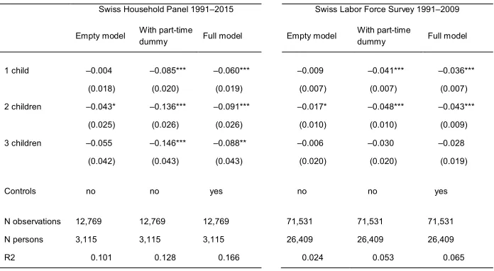
Table A-3: Fixed-effects linear regression on (log) hourly wages of women Swiss Household Panel 1991‒2015 Swiss Labor Force Survey 1991‒2009
Empty model With part-time
dummy Full model Empty model
With part-time
dummy Full model
1 child ‒0.004 ‒0.085*** ‒0.060*** ‒0.009 ‒0.041*** ‒0.036***
(0.018) (0.020) (0.019) (0.007) (0.007) (0.007)
2 children ‒0.043* ‒0.136*** ‒0.091*** ‒0.017* ‒0.048*** ‒0.043***
(0.025) (0.026) (0.026) (0.010) (0.010) (0.009)
3 children ‒0.055 ‒0.146*** ‒0.088** ‒0.006 ‒0.030 ‒0.028
(0.042) (0.043) (0.043) (0.020) (0.020) (0.019)
Controls no no yes no no yes
N observations 12,769 12,769 12,769 71,531 71,531 71,531
N persons 3,115 3,115 3,115 26,409 26,409 26,409
R2 0.101 0.128 0.166 0.024 0.053 0.065
Note: Coefficients are for the female labor force. All models include age (in years) and calendar years. The full model is shown in Table A-3 in the appendix. Clustered standard errors in parentheses.
Table A-4: Fixed-effect linear regression on (log) hourly wages of women
Note: Clustered standard errors in parentheses. *** p<0.01, ** p<0.05, * p<0.1. Coefficients are for the female labor force, aged 20‒ 50. All models include age in years and calendar years and, for the SLFS, a dummy variable for 13 different economic sectors and 9 ISCO 1-digit groups (not shown).
SHP 1999‒2015 SLFS 1991‒2009
1 child ‒0.060*** ‒0.036***
(0.019) (0.007)
2 children ‒0.091*** ‒0.043***
(0.026) (0.009)
3 children ‒0.088** ‒0.028
(0.043) (0.019)
Part-time 0.180*** 0.136***
(0.013) (0.005)
Years (SHP) / level (SLFS) of 0.022*** 0.011***
Education (0.005) (0.003)
% female in occupation 0.001 ‒0.012
(0.038) (0.019)
Public sector 0.040*** 0.008
(0.011) (0.032)
Firm size 0.010*** 0.003***
(0.002) (0.001)
Supervision 0.024*** 0.017***
(0.007) (0.003)
Occupational prestige 0.004***
(0.001)
Work experience (SHP) / 0.005 0.006***
Tenure (SLFS) (0.005) (0.002)
Job change last year ‒0.038
(0.029)
Employer change last year 0.015
(0.010)
Fixed-term job ‒0.121*** ‒0.047***
(0.022) (0.008)
Inadequate qualification ‒0.061*** (0.018)
Overqualified ‒0.041***
(0.009)
Underqualified ‒0.023
(0.023)
Training1 0.016** 0.000
(0.007) (0.002)
Training2 0.021***
(0.008)
Married ‒0.046*** ‒0.013**
(0.014) (0.005)
Hours of housework ‒0.002***
(0.001)
External childcare 0.010
(0.010)
Constant 2.348*** 3.041***
(0.116) (0.150)
N observations 12,769 71,531
N persons 3,115 26,409
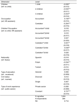
Table A-5: Wage recommendations for women depending on the number of children they have (factorial survey experiment)
Dimension Level
Children 1 child ‒0.026**
(ref: no child) (0.012)
2 children ‒0.030***
(0.011)
3 children ‒0.033**
(0.014)
Occcupation Accountant 0.159***
(ref: HR assistant) (0.014)
Caretaker ‒0.204***
(0.015)
Children*Occupation Accountant*1child 0.018
(ref: no child, HR assistant) (0.017)
Accountant*2child 0.010 (0.017) Accountant*3child 0.027
(0.020)
Caretaker*1child 0.041**
(0.018)
Caretaker*2child 0.038**
(0.017)
Caretaker*3child 0.026
(0.019)
Nationality Spanish ‒0.019
(ref: Swiss) (0.014)
Polish ‒0.034***
(0.011)
Turkish ‒0.014
(0.012)
Type of education General 0.006
(ref : vocational) (0.009)
Civil status Divorced 0.012
(ref : married) (0.010)
Single 0.007
(0.010)
Type of work experience Private sector ‒0.006
(ref : public sector) (0.008)
Constant 8.727***
(0.014)
N vignettes 1,644
N respondents 385
R2 0.712
Table A-6: Wage recommendations for women by respondent gender (factorial survey experiment)
Female respondents Male respondents
Children 1 child ‒0.038** ‒0.023
(ref: no child) (0.018) (0.016)
2 children ‒0.038** ‒0.027*
(0.016) (0.015)
3 children ‒0.044** ‒0.031*
(0.021) ‒0.023
Occcupation Accountant 0.155*** 0.157***
(ref: HR assistant) (0.021) (0.019)
Caretaker ‒0.214*** ‒0.196***
(0.021) (0.023)
Children*Occupation Accountant*1child 0.047* 0.001
(ref: no child, (0.026) (0.022)
HR assistant) Accountant*2child 0.008 0.025
(0.024) (0.026)
Accountant*3child 0.023 0.044
(0.029) (0.027)
Caretaker*1child 0.065** 0.021
(0.026) (0.025)
Caretaker*2child 0.043** 0.036
(0.022) (0.027)
Caretaker*3child 0.020 0.041
(0.026) (0.030)
Additional controls yes Yes
Constant 8.723*** 8.742***
(0.020) (0.016)
N vignettes 918 609
N respondents 203 129
R2 0.702 0.750
Notes: Respondent fixed-effects regressions on (log) wages for women aged 35 to 50. Clustered standard errors in parentheses. Additional controls include: civil status, nationality, type of education, type of work experience.