VOLUME 38, ARTICLE 18, PAGES 429
,
450
PUBLISHED 31 JANUARY 2018
http://www.demographic-research.org/Volumes/Vol38/18/ DOI: 10.4054/DemRes.2018.38.18
Research Article
Neighborhoods and mortality in Sweden:
Is deprivation best assessed nationally or
regionally?
Daniel Oudin Åström
Paul W. Franks
Kristina Sundquist
© 2018 Daniel Oudin Åström, Paul W. Franks & Kristina Sundquist.
This open-access work is published under the terms of the Creative Commons Attribution 3.0 Germany (CC BY 3.0 DE), which permits use, reproduction, and distribution in any medium, provided the original author(s) and source are given credit.
1 Introduction 430
2 Methods 432
2.1 Data sources 432
2.2 Statistical analyses 433
3 Results 435
4 Discussion 439
5 Strengths and limitations 442
6 Conclusion 443
7 Acknowledgments 443
References 444
Neighborhoods and mortality in Sweden:
Is deprivation best assessed nationally or regionally?
Daniel Oudin Åström1
Paul W. Franks2
Kristina Sundquist3
Abstract
BACKGROUND
The association between neighborhood deprivation and mortality is well established, but knowledge about whether deprivation is best assessed regionally or nationally is scarce.
OBJECTIVE
The present study aims to examine whether there is a difference in results when using national and county-specific neighborhood deprivation indices and whether the level of urbanization modifies the association between neighborhood deprivation and mortality. METHODS
We collected data on the entire population aged above 50 residing in the 21 Swedish counties on January 1, 1990, and followed them for mortality due to all causes and for coronary heart disease. The association between neighborhood deprivation and mortality was assessed using Cox regression, assuming proportional hazards with attained age as an underlying variable, comparing the 25% most deprived neighborhoods with the 25% most affluent ones within each region, and using both the national and the county-specific indices. The potential interactions were also assessed. RESULTS
The choice of a national or a county-specific index did not affect the estimates to a large extent. The effect of neighborhood deprivation on mortality in metropolitan regions (hazard ratio: 1.21 [1.20–1.22]) was somewhat higher than that in the more rural southern (HR: 1.16 [1.15–1.17]) and northern regions (HR: 1.11 [1.09–1.12]).
1 Center for Primary Health Care Research, Department of Clinical Sciences Malmö, Lund University,
Malmö, Sweden. Email:[email protected].
CONCLUSION
Our data indicates that the choice of a national or a county-specific deprivation index does not influence the results to a significant extent, but may be of importance in large metropolitan regions. Furthermore, the strength of the association between neighborhood deprivation and mortality is somewhat greater in metropolitan areas than in more rural southern and northern areas.
1. Introduction
The overall purpose of the study was to examine whether the well-known association between neighborhood deprivation and mortality differs depending on whether deprivation is assessed at the national or the county level, as well as to examine whether these associations vary between regions (metropolitan vs. rural, north vs. south).
The association between neighborhood deprivation, mortality, and impaired health is well established. For example, associations between neighborhood deprivation and mortality due to all causes and cardiovascular mortality in addition to cardiovascular morbidity and poor overall health have been reported (Chaix 2009; Cummins et al. 2007; Diez-Roux et al. 1997; Diez-Roux 2001; Diez-Roux et al. 2001; Diez-Roux et al. 2016; Meijer et al. 2012; Pickett and Pearl 2001). Several studies conducted in Sweden have reported similar findings: For example, coronary heart disease (CHD) incidence rates as well as case fatalities were higher in deprived neighborhoods than in wealthier neighborhoods (Winkleby, Sundquist, and Cubbin 2007; Chaix, Rosvall, and Merlo 2007; Carlsson et al. 2016; Oudin Åström, Sundquist and Sundquist 2018). Another Swedish study reported that individuals with diabetes residing in deprived neighborhoods had higher odds of being hospitalized for CHD than those who resided in wealthy neighborhoods (Chaikiat et al. 2012). The associations between neighborhood factors and health-related outcomes, including mortality, have mostly remained significant after taking individual factors, including socioeconomic status, into account (Diez-Roux et al. 2001; Pickett and Pearl 2001; Sundquist, Malmström, and Johansson 2004).
In the United States, Chetty et al. (2016) recently demonstrated that higher individual income was associated with greater longevity, with increasing differences across income groups over time (Chetty et al. 2016). These previous studies suggest that health policies need to focus on both individuals and neighborhoods.
However, most neighborhood studies in industrialized countries have used relative measures of neighborhood deprivation. Although most people in industrialized countries have their basic needs covered, associations between deprivation, mortality, and health-related outcomes still exist. Marmot (2004) showed the effect of social status on the heart disease risk in his famous studies of Whitehall civil servants (Marmot 2004). Although basic needs were met for all, those with a higher rank or social status had better health prospects and life expectancy, even when CHD risk factors such as smoking and cholesterol were factored out. These effects may be caused by relative rather than absolute deprivation, as individuals tend to compare their own situation with that of the people around them (Walker and Pettigrew 1984). We therefore hypothesize that the effect on mortality of the relative level of neighborhood deprivation may differ when the relative deprivation is assessed at the county rather than the national level (the latter being the most common approach in previous neighborhood studies).
We also hypothesize that the effect on mortality of neighborhood deprivation may differ between regions. For example, in a study that examined trends in rural vs. urban disparities in the United States between 1969 and 2009, those residing in metropolitan regions experienced larger reductions in mortality than those residing in more rural regions (Singh and Siahpush 2014). Similar results have been shown in other studies from the United States (Kulshreshtha et al. 2014) and Sweden (Winkleby, Sundquist, and Cubbin 2007). A recent study from the United Kingdom, covering the period 1965 to 2010, found excess mortality rates remained consistent over time in the five northernmost compared to the four southernmost Government Office Regions in England (Buchan et al. 2017). In Sweden, life expectancy may differ by up to two and a half years depending on county of residence (Statistics Sweden 2017).
The specific aims of the present study were:
1. To investigate the association between neighborhood deprivation and mortality due to all causes and to CHD using the neighborhood deprivation index (NDI) at both national and county-specific levels.
2. To examine whether the estimates differ when using an NDI at a national or a county level.
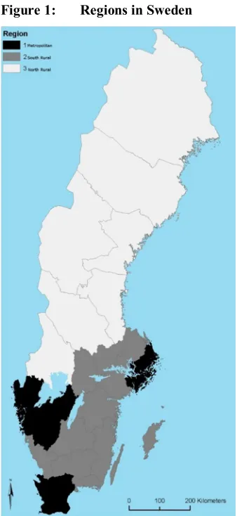
3. To investigate whether the effect on mortality of living in the most deprived areas is different in a metropolitan setting compared to more rural areas in southern and northern Sweden.
2. Methods
2.1 Data sources
Statistics Sweden provided individual-level demographic and socioeconomic data for the study population. This data consisted of the entire Swedish population aged above 50 residing in any of the 21 regions of Sweden on January 1, 1990. We chose the cut-off point of 50 years of age because mortality due to CHD is rare in younger populations (National Heart, Lung, and Blood Institute 2016). In addition, elderly frail people may be negatively affected by both individual socioeconomic status and level of neighborhood deprivation (Lang et al. 2009; Yen, Michael, and Perdue 2009).
During the study period (January 1, 1990, until December 31, 2013) we collected dates of fatal events due to all causes and, more specifically, fatalities due to a CHD-coded event (ICD-9: 410–414; ICD-10: I20–I25). Each individual was followed until date of death, end of study, or loss to follow-up (indicating that he or she had moved away from the area of residence they were registered at in 1990), whichever came first.
The home addresses of all Swedish adults have been geocoded to represent small geographic units. These neighborhood areas, known as small area market statistics (SAMS), have an average population of 1,000 to 2,000 inhabitants. SAMS were used as proxies for neighborhoods, as described elsewhere (Carlsson et al. 2016; Winkleby, Sundquist, and Cubbin 2007). Approximately 90% of women and men lived in the same SAMS neighborhood over the course of the study: that is, from the start of the study to either death or the end of the study.
(Winkleby, Sundquist, and Cubbin 2007). In the present study, higher scores indicate more affluent neighborhoods, whereas lower scores indicate more deprived neighborhoods. For each separate region, as well as for Sweden as a whole, we calculated the 25th, 50th, and 75th percentiles of the NDI for the year 1990. We included data from 8,104 SAMS in the present study (excluding SAMS with fewer than 50 inhabitants).
2.2 Statistical analyses
The association between neighborhood deprivation and mortality was assessed using Cox proportional hazards regression, with attained age as the underlying time variable. The analyses compared the 25% most deprived SAMS to the 25% most affluent SAMS within each region, using the NDI calculated on a national as well as a regional level. Before calculating a region-specific index, we investigated the presence of a statistical interaction between region and NDI in our Cox proportional hazard regression model. Our data suggested strong evidence for such an interaction term.
Model 1: First, we included only NDI in the model. We ran this model using the NDI calculated for Sweden, as well as separately for each county. This allowed us to investigate differences in the association when using the index at both national and county-specific levels. We stratified the analyses on county of residence.
Model 2: Second, we adjusted Model 1 for putative confounders at an individual level. We included sex, educational attainment (three levels: ≤9 years [completion of compulsory school or less], 10–11 years [practical high school], and ≥12 years [theoretical high school and/or college]), recipient of social welfare (yes/no), and family income in Swedish kronor (SEK) (continuous variable).
Figure 1: Regions in Sweden
Formal tests for proportionality were performed by adding an interaction term between the logarithm of the time variable and neighborhood characteristics. The interactions were all statistically nonsignificant at the 5% level, indicating that the proportionality assumption with time was not violated.
To additionally evaluate if using a national- or a county-level index resulted in an observed difference in the association between neighborhood deprivation and mortality, we calculated a Z-score and corresponding p-value. To be conservative we used the Bonferroni method of p-value correction to compensate for multiple comparisons (Bland and Altman 1995).
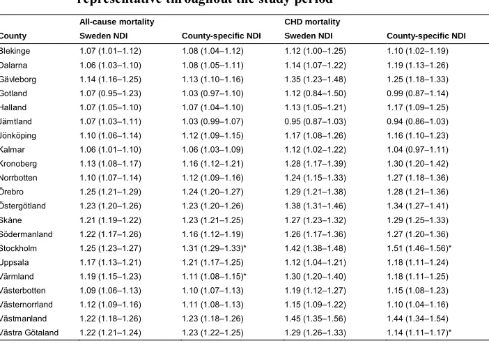
As a sensitivity analysis, rather than censoring those moving to a new SAMS of residence, we assumed the SAMS of residence in 1990 to be representative for the entire period the individual remained in the study: that is, until death or the end of the study. The results from the sensitivity analysis were almost identical (see Table A-1).
3. Results
Table 1: Population size, follow-up time, and distribution of the
sociodemographic variables by the 21 counties in Sweden at baseline
County Population size
Pop. 25%
deprived1 Pop. 25%affluent2 %Women Age medianand IQR3 Incomemedian and IQR4 Follow-up timemedian and IQR
Blekinge 53,033 12,105 (23) 14,189 (27) 53 66 (57–74) 716 (582–936) 18 (9–24)
Dalarna 99,728 25,622 (26) 23,830 (24) 54 66 (58–74) 728 (594–936) 17 (9–24)
Gävleborg 101,771 25,275 (25) 18,614 (18) 54 66 (58–74) 734 (603–939) 17 (9–24)
Gotland 17,947 2,873 (16) 6,534 (36) 53 66 (57–74) 686 (544–882) 18 (9–24)
Halland 80,331 15,518 (19) 22,632 (28) 53 65 (57–74) 751 (600–977) 19 (10–24)
Jämtland 47,513 7,565 (16) 13,369 (28) 52 67 (58–75) 710 (576–924) 17 (8–24)
Jönköping 107,441 20,116 (19) 24,822 (23) 54 66 (58–74) 731 (597–944) 18 (9–24)
Kalmar 84,629 14,056 (17) 20,462 (24) 53 66 (58–75) 704 (573–915) 17 (9–24)
Kronoberg 58,615 12,597 (21) 11,736 (20) 53 66 (58–75) 734 (579–947) 18 (9–24)
Norrbotten 83,608 13,025 (16) 17,817 (21) 52 64 (56–73) 775 (618–995) 19 (10–24)
Örebro 92,028 26,700 (29) 18,378 (20) 54 67 (58–75) 728 (606–944) 18 (9–24)
Östergötland 131,212 33,345 (25) 26,247 (20) 54 66 (58–74) 737 (603–950) 17 (9–24)
Skåne 351,853 88,170 (25) 71,613 (20) 55 66 (57–74) 763 (618–992) 18 (9–24)
Södermanland 83,559 22,860 (27) 14,444 (17) 54 66 (57–74) 763 (621–977) 18 (9–24)
Stockholm 457,021 128,780 (28) 91,814 (20) 56 65 (57–73) 900 (701–1,149) 18 (9–24)
Uppsala 71,027 19,439 (27) 15,438 (22) 54 65 (57–74) 781 (615–1,016) 19 (10–24)
Värmland 100,757 23,384 (23) 19,113 (19) 54 66 (58–74) 728 (594–941) 19 (9–24)
Västerbotten 79,887 12,170 (15) 19,508 (24) 53 65 (57–73) 751 (600–968) 17 (9–24)
Västernorrland 91,599 22,467 (25) 23,463 (26) 53 66 (58–74) 751 (600–974) 18 (9–24)
Västmanland 79,745 22,337 (28) 15,634 (20) 54 65 (57–73) 775 (627–995) 17 (9–24)
Västra Götaland 463,969 98,160 (21) 95,787 (21) 54 66 (58–74) 754 (612–974) 19 (10–24)
Sweden 2,737,273 646,564 (24) 585,444 (21) 54 66 (57–74) 769 (618–974) 18 (9–24) Note:1 Size and percentage of the population residing in the 25% most deprived neighborhoods (county-specific neighborhood
deprivation index).2 Size and percentage of the population residing in the 25% most affluent neighborhoods (county-specific
neighborhood deprivation index).3 IQR = interquartile range.4 Family income in thousands of Swedish kronor.
A total of 54% of the entire study population was female. At the time of inclusion in the study, the median age in the total population was 66 years (IQR = 57–74). The median annual family income was 900,000 SEK in Stockholm (highest) and 686,000 SEK in Gotland (lowest) and varied between 704,000 and 781,000 SEK in the other 19 counties. The median follow-up time in the 21 counties varied between 17 and 19 years. In the total population, 65% (N = 1,779,552) of the people died during the course of the study. The median follow-up time was 18 years.
Figure 2: Medians of the neighborhood deprivation index for Sweden and the counties in 1990
confidence level increased to 10%. Table A-2 shows the crude HRs, which were generally higher than in the adjusted HRs shown in Table 2.
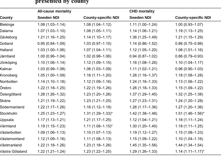
Table 2: Adjusted hazard ratios and 95% confidence intervals for all-cause mortality and mortality due to coronary heart disease (CHD), presented by county
All-cause mortality CHD mortality
County Sweden NDI County-specific NDI Sweden NDI County-specific NDI
Blekinge 1.08 (1.03–1.14) 1.08 (1.04–1.12) 1.11 (1.00–1.24) 1.00 (0.93–1.07)
Dalarna 1.07 (1.03–1.10) 1.08 (1.05–1.11) 1.14 (1.06–1.21) 1.19 (1.13–1.25)
Gävleborg 1.21 (1.16–1.25) 1.14 (1.10–1.17) 1.36 (1.25–1.49) 1.21 (1.15–1.29)
Gotland 0.95 (0.84–1.09) 1.03 (0.97–1.10) 1.14 (0.86–1.52) 0.86 (0.75–0.98)
Halland 1.03 (1.00–1.06) 1.07 (1.04–1.11) 1.12 (1.05–1.20) 1.08 (1.01–1.16)
Jämtland 1.00 (0.96–1.04) 1.02 (0.98–1.06) 0.94 (0.87–1.02) 0.86 (0.79–0.93)
Jönköping 1.10 (1.06–1.14) 1.12 (1.09–1.15) 1.16 (1.08–1.26) 1.10 (1.04–1.17)
Kalmar 1.03 (0.99–1.08) 1.06 (1.03–1.09) 1.11 (1.02–1.21) 0.96 (0.90–1.03)
Kronoberg 1.05 (1.00–1.09) 1.16 (1.11–1.20) 1.26 (1.16–1.37) 1.18 (1.08–1.28)
Norrbotten 1.14 (1.10–1.18) 1.12 (1.09–1.16) 1.24 (1.16–1.33) 1.13 (1.06–1.22)
Örebro 1.22 (1.18–1.25) 1.22 (1.19–1.26) 1.26 (1.18–1.33) 1.15 (1.09–1.22)
Östergötland 1.28 (1.26–1.32) 1.23 (1.20–1.26) 1.37 (1.29–1.45) 1.32 (1.25–1.38)
Skåne 1.21 (1.19–1.22) 1.23 (1.21–1.25) 1.27 (1.23–1.31) 1.24 (1.20–1.28)
Södermanland 1.22 (1.17–1.26) 1.16 (1.12–1.19) 1.26 (1.17–1.36) 1.27 (1.20–1.36)
Stockholm 1.25 (1.23–1.27) 1.31 (1.29–1.33)* 1.42 (1.38–1.48) 1.51 (1.46–1.56)*
Uppsala 1.17 (1.13–1.21) 1.21 (1.17–1.25) 1.12 (1.04–1.21) 1.18 (1.11–1.24)
Värmland 1.19 (1.15–1.23) 1.11 (1.08–1.15)* 1.30 (1.20–1.40) 1.18 (1.11–1.25)
Västerbotten 1.09 (1.06–1.13) 1.10 (1.07–1.13) 1.19 (1.12–1.27) 1.15 (1.08–1.23)
Västernorrland 1.12 (1.09–1.16) 1.11 (1.08–1.13) 1.15 (1.09–1.22) 1.10 (1.04–1.16)
Västmanland 1.22 (1.18–1.26) 1.23 (1.18–1.26) 1.45 (1.35–1.56) 1.44 (1.34–1.54)
Västra Götaland 1.22 (1.21–1.24) 1.23 (1.22–1.25) 1.29 (1.26–1.33) 1.14 (1.11–1.17)*
Note: Model adjusted for income, education, sex, and if recipient of social welfare. NDI = neighborhood deprivation index. * indicates non-overlapping confidence intervals between the national and county-specific indices of deprivation after Bonferroni adjustment for multiplicity issues.
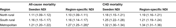
was 1.21 (95% CI: 1.20–1.22) and 1.27 (95% CI: 1.25–1.28). For CHD mortality, the corresponding HRs were 1.32 (95% CI: 1.30–1.34) for the national NDI and 1.34 (95% CI: 1.31–1.36) for the metropolitan-specific NDI respectively.
Table 3: Adjusted hazard ratios and 95% confidence intervals for all-cause mortality and mortality due to coronary heart disease (CHD), presented by region
All-cause mortality CHD mortality
Region Sweden NDI Region-specific NDI Sweden NDI Region-specific NDI
North rural 1.11 (1.09–1.12) 1.10 (1.09–1.11) 1.18 (1.15–1.21) 1.19 (1.16–1.21)
South rural 1.16 (1.15–1.17) 1.16 (1.14–1.17) 1.25 (1.22–1.28) 1.21 (1.19–1.24)
Metropolitan 1.21 (1.20–1.22) 1.27 (1.25–1.28)* 1.32 (1.30–1.34) 1.34 (1.31–1.36)
Note: Model adjusted for income, education, sex, and if recipient of social welfare. NDI = neighborhood deprivation index. * indicates non-overlapping confidence intervals between the national and regional indices of deprivation.
4. Discussion
The present study shows that there are associations in most counties between neighborhood deprivation and mortality due to all causes and to CHD. These associations were found using the NDIs derived at both national and county levels. In only one county, Stockholm, was a significant difference (95% CI and accounting for multiple testing) observed between the HRs for all-cause mortality when using the national NDI and the county-specific NDI. For CHD mortality, this was the case for the counties of Västra Götaland and Stockholm, the two most populous counties. The strength of the association between neighborhood deprivation and all-cause mortality, as well as CHD mortality, was greater in the metropolitan than in the more rural areas in the southern and northern regions. This was the case when using both the national and the region-specific NDIs.
The magnitudes of the increased risk of mortality, both all-cause and due to CHD, are in accordance with previous findings. Increased mortality due to all causes has been previously reported among individuals residing in areas with low social capital (odds ratio after adjustments 1.27 95% CI 1.25–1.29) (Sundquist et al. 2014). Regarding CHD mortality, Winkleby, Sundquist, and Cubbin (2007) found an increased risk for both men, HR: 1.36 (1.22–1.52), and women, HR: 1.33 (1.08–1.65), among those residing in a neighborhood defined as being highly deprived as compared to a low deprivation equivalent (Winkleby, Sundquist, and Cubbin 2007). Wändell et al. (2016) recently found that individuals diagnosed with atrial fibrillation who resided in a deprived neighborhood had the highest mortality risk due to all causes (HR: 1.49 95% CI 1.13– 1.96) (Wändell et al. 2016).
Overall, we found that the mortality risks were similar in most counties when comparing the estimates derived from NDIs at both national and county-specific levels. This means that for most counties it is not necessary to calculate a county-specific NDI instead of using the readily available national NDI. Thus, our data does not support our hypothesis that a county-specific index may better reflect relevant socioeconomic differences associated with mortality than a nationally derived NDI, with some exceptions. A possible explanation for our finding may be that Sweden is a relatively homogeneous country from a socioeconomic perspective. Our hypothesis was, however, confirmed in two counties, Västra Götaland and Stockholm. There the magnitude of the estimated HRs was significantly higher (95% CI and accounting for multiple testing) for both all-cause mortality and CHD mortality when using the county-specific NDI. An opposite pattern was observed in the county of Värmland: when using the nationally derived NDI, the magnitude of the estimated HRs was significantly higher for all-cause mortality and also tended to be higher for CHD mortality, although the results did not remain significant for Värmland after adjusting for multiple testing. A possible explanation, albeit not robust in Värmland when accounting for multiple testing, is that when these counties, representing the most affluent (Stockholm) and the most deprived (Värmland), are assessed by the NDI, we will be comparing the populations within each county with two different reference populations although the same deprivation index is being used at both national and county levels. Furthermore, the pattern of a potentially different effect on mortality when the median of the county-specific index differs from the median of the national index is not consistent in our material, which supports our conclusion that the choice of NDI, national or county-specific, may be of importance only in large metropolitan regions.
life expectancy was approximately two years for women and two and a half years for men (Statistics Sweden 2017). There are also differences in the NDI between counties that reflect the socioeconomic differences within Sweden. The NDI is based on four variables: low educational status, low income, unemployment, and receiving social welfare (Winkleby, Sundquist, and Cubbin 2007). Some of the observed differences in mortality between the most deprived counties and the most affluent counties may, however, also be affected by other differences between regions, such as level of urbanization and access to services and resources.
Another important finding of the present study is that the strength of the association between neighborhood deprivation and all-cause as well as CHD mortality was greater in the metropolitan than in the more rural areas whether using the national or the county-specific NDI. This means that neighborhood deprivation may have a more detrimental effect on life expectancy in metropolitan than in more rural areas. Our findings partially corroborate those of Winkleby, Sundquist, and Cubbin (2007), where urban areas were found to have higher mortality rates than midsized towns and smaller cities (Winkleby, Sundquist, and Cubbin 2007). However, to the best of our knowledge, this study is the first that covers an entire population to present evidence of a potentially stronger effect of neighborhood deprivation in metropolitan regions. One possible explanation for our findings is that relative poverty in the metropolitan regions might transfer to larger absolute differences in neighborhood deprivation in these regions. We hypothesized that the association between neighborhood deprivation and mortality would differ between urban and rural regions. A Canadian study compared survival inequalities using both an area-based index and an individual index of deprivation. The authors concluded that survival inequalities in rural areas were lower than in urban areas when using an area-based index but of a similar magnitude when using an individual index (Pampalon, Hamel, and Gamache 2010), which is consistent with the findings of our study.
5. Strengths and limitations
The main strength of the current study is that it covers the entire population aged above 50 residing in Sweden at the start of follow-up in 1990. Another strength is the investigation of both all-cause mortality and mortality due to CHD. The validity of the Swedish Cause of Death registers can be considered to be high and thus misclassification of deaths due to CHD should be limited (National Board of Health and Welfare 2017). Furthermore, the nationwide registers used in the study are almost complete, so any loss to follow-up is limited. The consistent definition of the areas that we studied, both geographically and over time, is another strength that minimized bias due to the modifiable area unit problem. Such bias may arise when the aggregation of events into geographic areas is dependent of the researcher’s choice (Wong 2009). We used the same geographic boundaries to define the counties each year of the study, when using both the national and the regional NDIs. There were only slight changes in the definitions of Swedish counties during the course of the study. For instance, in 1998 the two southernmost counties were merged into one, resulting in the county of Scania. We used the merged two counties to define the county of Scania throughout the entire study period.
6. Conclusion
Despite the observed differences in the median of the NDI between counties, our data suggests that the choice of NDI, national or county-specific, may be of importance only in large metropolitan regions. Furthermore, neighborhood deprivation may have a greater detrimental effect on life expectancy in metropolitan than in more rural areas. Future studies should examine which mechanisms underlying the association between neighborhood deprivation and mortality are at work in metropolitan regions.
7. Acknowledgments
References
Bland, J.M. and Altman, D.G. (1995). Multiple significance tests: The Bonferroni method.BMJ 310(6973): 170.doi:10.1136/bmj.310.6973.170.
Bozdogan, H. (1987). Model selection and Akaike’s information criterion (AIC): The general theory and its analytical extensions. Psychometrika 52(3): 345–370.
doi:10.1007/BF02294361.
Buchan, I.E., Kontopantelis, E., Sperrin, M., Chandola, T., and Doran, T. (2017). North–South disparities in English mortality 1965–2015: Longitudinal population study.Journal of Epidemiology and Community Health 71: 928–936.
doi:10.1136/jech-2017-209195.
Carlsson, A.C., Li, X., Holzmann, M.J., Wändell, P., Gasevic, D., Sundquist, J., and Sundquist, K. (2016). Neighbourhood socioeconomic status and coronary heart disease in individuals between 40 and 50 years. Heart 102(10): 775–782.
doi:10.1136/heartjnl-2015-308784.
Chaikiat, Å., Li, X., Bennet, L., and Sundquist, K. (2012). Neighborhood deprivation and inequities in coronary heart disease among patients with diabetes mellitus: A multilevel study of 334,000 patients. Health and Place 18(4): 877–882.
doi:10.1016/j.healthplace.2012.03.003.
Chaix, B. (2009). Geographic life environments and coronary heart disease: A literature review, theoretical contributions, methodological updates, and a research agenda. Annual Review of Public Health 30: 81–105. doi:10.1146/annurev. publhealth.031308.100158.
Chaix, B., Rosvall, M., and Merlo, J. (2007). Neighborhood socioeconomic deprivation and residential instability: Effects on incidence of ischemic heart disease and survival after myocardial infarction.Epidemiology 18(1): 104–111.doi:10.1097/ 01.ede.0000249573.22856.9a.
Chetty, R., Stepner, M., Abraham, S., Lin, S., Scuderi, B., Turner, N., Bergeron, A., and Cutler, D. (2016). The association between income and life expectancy in the United States, 2001–2014. JAMA 315(16): 1750–1766.doi:10.1001/jama.2016. 4226.
Cummins, S., Curtis, S., Diez-Roux, A.V., and Macintyre, S. (2007). Understanding and representing ‘place’ in health research: A relational approach.Social Science
Diez-Roux, A.V. (2001). Investigating neighborhood and area effects on health.
American Journal of Public Health 91(11): 1783–1789. doi:10.2105/AJPH.91.
11.1783.
Diez-Roux, A.V., Merkin, S.S., Arnett, D., Chambless, L., Massing, M., Nieto, F.J., Sorlie, P., Szklo, M., Tyroler, H.A., and Watson, R.L. (2001). Neighborhood of residence and incidence of coronary heart disease. New England Journal of
Medicine 345(2): 99–106.doi:10.1056/NEJM200107123450205.
Diez-Roux, A.V., Mujahid, M.S., Hirsch, J.A., Moore, K., and Moore, L.V. (2016). The impact of neighborhoods on CV risk. Global Heart 11(3): 353–363.
doi:10.1016/j.gheart.2016.08.002.
Diez-Roux, A.V., Nieto, F.J., Muntaner, C., Tyroler, H.A., Comstock, G.W., Shahar, E., Cooper, L.S., Watson, R.L., and Szklo, M. (1997). Neighborhood environments and coronary heart disease: A multilevel analysis. American
Journal of Epidemiology 146(1): 48–63. doi:10.1093/oxfordjournals.aje.
a009191.
Elgar, F.J., Xie, A., Pförtner, T.K., White, J., and Pickett, K.E. (2016). Relative deprivation and risk factors for obesity in Canadian adolescents.Social Science
and Medicine 152: 111–118.doi:10.1016/j.socscimed.2016.01.039.
Kulshreshtha, A., Goyal, A., Dabhadkar, K., Veledar, E., and Vaccarino, V. (2014). Urban–rural differences in coronary heart disease mortality in the United States: 1999–2009. Public Health Reports 129(1): 19–29. doi:10.1177/ 003335491412900105.
Lang, I.A., Hubbard, R.E., Andrew, M.K., Llewellyn, D.J., Melzer, D., and Rockwood, K. (2009). Neighborhood deprivation, individual socioeconomic status, and frailty in older adults.Journal of the American Geriatrics Society 57(10): 1776– 1780.doi:10.1111/j.1532-5415.2009.02480.x.
Marmot, M. (2004). Status syndrome.Significance 1(4): 150–154. doi:10.1111/j.1740-9713.2004.00058.x.
Meijer, M., Röhl, J., Bloomfield, K., and Grittner, U. (2012). Do neighborhoods affect individual mortality? A systematic review and meta-analysis of multilevel studies. Social Science and Medicine 74(8): 1204–1212. doi:10.1016/j. socscimed.2011.11.034.
National Heart, Lung, and Blood Institute (2016). Coronary heart disease risk factors [electronic resource]. Bethesda: National Heart, Lung and Blood Institute.
www.nhlbi.nih.gov/health/health-topics/topics/hd/atrisk.
Oudin Åström, D., Sundquist, J., and Sundquist, K. (2018). Differences in declining mortality rates due to coronary heart disease by neighbourhood deprivation.
Journal of Epidemiology and Community Health.
doi:10.1136/jech-2017-210105.
Pampalon, R., Hamel, D., and Gamache, P. (2010). Health inequalities in urban and rural Canada: Comparing inequalities in survival according to an individual and area-based deprivation index. Health and Place 16: 416–420. doi:10.1016/j. healthplace.2009.11.012.
Pickett, K.E. and Pearl, M. (2001). Multilevel analyses of neighbourhood socioeconomic context and health outcomes: A critical review. Journal of
Epidemiology and Community Health 55(2): 111–122. doi:10.1136/jech.55.
2.111.
Singh, G.K. and Siahpush, M. (2014). Widening rural–urban disparities in all-cause mortality and mortality from major causes of death in the USA, 1969–2009.
Journal of Urban Health 91(2): 272–292.doi:10.1007/s11524-013-9847-2.
Statistics Sweden (2017). Återstående medellivslängd länsvis efter kön. Femårsperioder 1966‒1970 ‒ 2012‒2016. Stockholm: Statistics Sweden. http://www.statistik databasen.scb.se/pxweb/sv/ssd/START__BE__BE0101__BE0101I/Medellivslan gdL/?rxid=f45f90b6-7345-4877-ba25-9b43e6c6e299.
Sundquist, K., Malmström, M., and Johansson, S.-E. (2004). Neighborhood deprivation and incidence of coronary heart disease: A multilevel study of 2.6 million women and men in Sweden. Journal of Epidemiology and Community Health
58: 71–77.doi:10.1136/jech.58.1.71.
Sundquist, K., Hamano, T., Li, X., Kawakami, N., Shiwaku, K., and Sundquist, J. (2014). Linking social capital and mortality in the elderly: A Swedish national cohort study. Experimental Gerontology 55: 29–36. doi:10.1016/j.exger.2014. 03.007.
Walker, I. and Pettigrew, T.F. (1984). Relative deprivation theory: An overview and conceptual critique. British Journal of Social Psychology 23(4): 301–310.
doi:10.1111/j.2044-8309.1984.tb00645.x.
atrial fibrillation: A cohort study of patients treated in primary care in Sweden.
International Journal of Cardiology 202: 776–781.doi:10.1016/j.ijcard.2015.09. 027.
Winkleby, M., Sundquist, K., and Cubbin, C. (2007). Inequities in CHD incidence and case fatality by neighborhood deprivation. American Journal of Preventive
Medicine 32(2): 97–106.doi:10.1016/j.amepre.2006.10.002.
Wong, D. (2009). The modifiable areal unit problem (MAUP). In: Fotheringham, A.S. and Rogerson, P.A. (eds.). The SAGE handbook of spatial analysis. Thousand Oaks: Sage: 105–123.doi:10.4135/9780857020130.n7.
Appendix
Table A-1: Adjusted hazard ratios and 95% confidence intervals for all-cause mortality and mortality due to coronary heart disease (CHD), presented by county, assuming neighborhood of residence 1990 to be representative throughout the study period
All-cause mortality CHD mortality
County Sweden NDI County-specific NDI Sweden NDI County-specific NDI
Blekinge 1.07 (1.01–1.12) 1.08 (1.04–1.12) 1.12 (1.00–1.25) 1.10 (1.02–1.19)
Dalarna 1.06 (1.03–1.10) 1.08 (1.05–1.11) 1.14 (1.07–1.22) 1.19 (1.13–1.26)
Gävleborg 1.14 (1.16–1.25) 1.13 (1.10–1.16) 1.35 (1.23–1.48) 1.25 (1.18–1.33)
Gotland 1.07 (0.95–1.23) 1.03 (0.97–1.10) 1.12 (0.84–1.50) 0.99 (0.87–1.14)
Halland 1.07 (1.05–1.10) 1.07 (1.04–1.10) 1.13 (1.05–1.21) 1.17 (1.09–1.25)
Jämtland 1.07 (1.03–1.11) 1.03 (0.99–1.07) 0.95 (0.87–1.03) 0.94 (0.86–1.03)
Jönköping 1.10 (1.06–1.14) 1.12 (1.09–1.15) 1.17 (1.08–1.26) 1.16 (1.10–1.23)
Kalmar 1.06 (1.01–1.10) 1.06 (1.03–1.09) 1.12 (1.02–1.22) 1.04 (0.97–1.11)
Kronoberg 1.13 (1.08–1.17) 1.16 (1.12–1.21) 1.28 (1.17–1.39) 1.30 (1.20–1.42)
Norrbotten 1.10 (1.07–1.14) 1.12 (1.09–1.16) 1.24 (1.15–1.33) 1.27 (1.18–1.36)
Örebro 1.25 (1.21–1.29) 1.24 (1.20–1.27) 1.29 (1.21–1.38) 1.28 (1.21–1.36)
Östergötland 1.23 (1.20–1.26) 1.23 (1.20–1.26) 1.38 (1.31–1.46) 1.34 (1.27–1.41)
Skåne 1.21 (1.19–1.22) 1.23 (1.21–1.25) 1.27 (1.23–1.32) 1.29 (1.25–1.33)
Södermanland 1.22 (1.17–1.26) 1.16 (1.12–1.19) 1.26 (1.17–1.36) 1.27 (1.20–1.36)
Stockholm 1.25 (1.23–1.27) 1.31 (1.29–1.33)* 1.42 (1.38–1.48) 1.51 (1.46–1.56)*
Uppsala 1.17 (1.13–1.21) 1.21 (1.17–1.25) 1.12 (1.04–1.21) 1.18 (1.11–1.24)
Värmland 1.19 (1.15–1.23) 1.11 (1.08–1.15)* 1.30 (1.20–1.40) 1.18 (1.11–1.25)
Västerbotten 1.09 (1.06–1.13) 1.10 (1.07–1.13) 1.19 (1.12–1.27) 1.15 (1.08–1.23)
Västernorrland 1.12 (1.09–1.16) 1.11 (1.08–1.13) 1.15 (1.09–1.22) 1.10 (1.04–1.16)
Västmanland 1.22 (1.18–1.26) 1.23 (1.18–1.26) 1.45 (1.35–1.56) 1.44 (1.34–1.54)
Västra Götaland 1.22 (1.21–1.24) 1.23 (1.22–1.25) 1.29 (1.26–1.33) 1.14 (1.11–1.17)*
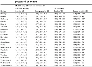
Table A-2: Crude hazard ratios and 95% confidence intervals for all-cause mortality and mortality due to coronary heart disease (CHD), presented by county
Model 1 (only NDI included in the model)
All-cause mortality CHD mortality
Region Sweden NDI County-specific NDI Sweden NDI County-specific NDI
Blekinge 1.42 (1.36–1.48) 1.18 (1.14–1.21)* 1.49 (1.35–1.64) 1.21 (1.14–1.29)*
Dalarna 1.35 (1.31–1.39) 1.29 (1.26–1.32) 1.48 (1.40–1.56) 1.42 (1.36–1.48)
Gävleborg 1.62 (1.56–1.67) 1.37 (1.33–1.40)* 1.92 (1.78–2.08) 1.54 (1.46–1.62)*
Gotland 1.16 (1.04–1.29) 1.09 (1.03–1.15) 1.27 (0.99–1.62) 1.06 (0.94–1.19)
Halland 1.38 (1.35–1.42) 1.37 (1.33–1.41) 1.55 (1.46–1.64) 1.56 (1.48–1.66)
Jämtland 1.36 (1.31–1.40) 1.29 (1.25–1.33) 1.23 (1.14–1.32) 1.19 (1.11–1.28)
Jönköping 1.43 (1.38–1.47) 1.34 (1.31–1.37)* 1.54 (1.44–1.65) 1.36 (1.30–1.43)
Kalmar 1.38 (1.34–1.43) 1.27 (1.24–1.31)* 1.47 (1.37–1.58) 1.32 (1.24–1.39)
Kronoberg 1.40 (1.36–1.45) 1.41 (1.36–1.45) 1.60 (1.49–1.72) 1.59 (1.49–1.71)
Norrbotten 1.47 (1.43–1.51) 1.36 (1.32–1.40)* 1.61 (1.51–1.71) 1.55 (1.46–1.65)
Örebro 1.42 (1.39–1.46) 1.37 (1.34–1.40) 1.49 (1.41–1.57) 1.42 (1.35–1.49)
Östergötland 1.66 (1.62–1.70) 1.59 (1.56–1.62)* 1.82 (1.74–1.91) 1.71 (1.64–1.79)
Skåne 1.54 (1.52–1.56) 1.51 (1.50–1.53) 1.71 (1.66–1.76) 1.64 (1.60–1.69)
Södermanland 1.68 (1.62–1.73) 1.58 (1.54–1.62)* 1.79 (1.67–1.91) 1.66 (1.57–1.76)
Stockholm 1.18 (1.16–1.19) 1.64 (1.62–1.66)* 1.32 (1.28–1.36) 1.90 (1.85–1.95)*
Uppsala 1.26 (1.23–1.30) 1.27 (1.24–1.31) 1.20 (1.13–1.28) 1.22 (1.15–1.29)
Värmland 1.75 (1.70–1.81) 1.46 (1.42–1.49)* 1.95 (1.82–2.08) 1.59 (1.52–1.68)*
Västerbotten 1.44 (1.40–1.48) 1.47 (1.42–1.51) 1.57 (1.48–1.66) 1.61 (1.51–1.71)
Västernorrland 1.46 (1.43–1.50) 1.42 (1.39–1.45) 1.53 (1.46–1.61) 1.51 (1.44–1.58)
Västmanland 1.52 (1.48–1.57) 1.56 (1.52–1.61) 1.77 (1.66–1.88) 1.83 (1.73–1.95)
Västra Götaland 1.46 (1.44–1.48) 1.43 (1.41–1.44)* 1.59 (1.55–1.63) 1.55 (1.51–1.59)