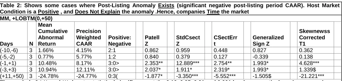
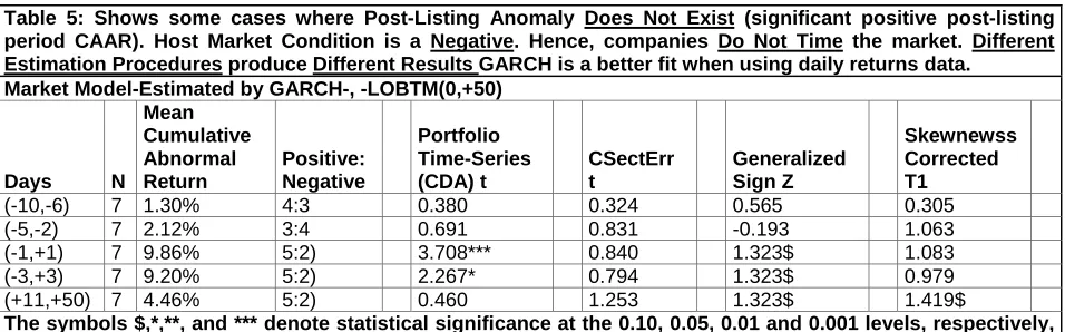
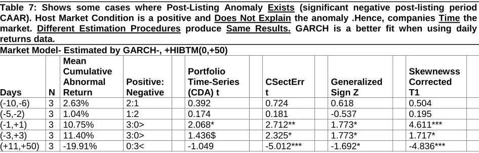
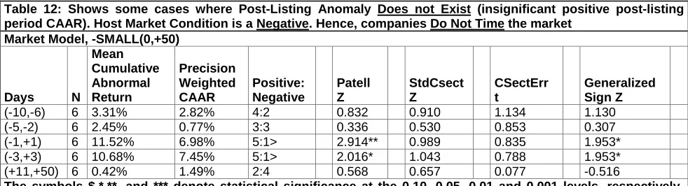
Does the choice of benchmarks matter?
The characteristic index vs. the market index
Moustafa Fadl
Finance Department, Old Dominion University, Norfolk, Virginia, USA
E-mail: [email protected], Tel: +1–757–472–7027;
ABSTRACT
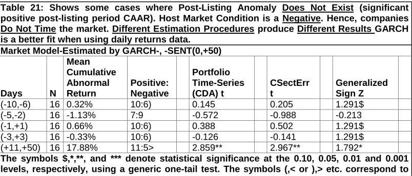
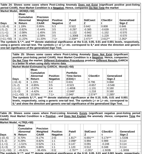
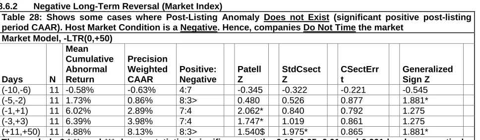
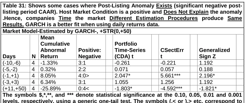
Previous research documented that soon after companies cross list, they achieve significant negative post-listing abnormal returns (the post-listing anomaly). The host market condition was the most recent satisfactory explanation for the sign, and the significance of the anomaly. Event studies are based on grouping companies by certain characteristics, as such, the choice of benchmarks affect the method of forming portfolios of companies, which in turn, affect the sign and the significance of the post-listing abnormal returns. The sample evidence shows for almost the different Characteristic Index benchmarks used, different estimation procedures neither changed the sign nor the significance of the post-listing abnormal returns. But, for almost the different Market Index benchmarks used, different estimation procedures changed the sign, and the significance of the post-listing abnormal returns. The GARCH estimation procedure is a better fit when using daily returns to estimate abnormal returns, and the Characteristic Index is a better fit when forming portfolios of companies based on certain characteristics. With either the Characteristic Index or the Market Index, some companies time the market before cross-listing, and they achieve significant negative post-listing abnormal returns. While, others who don‘t time the market, they achieve significant positive post–listing abnormal returns. The paper used an event study methodology and a wide variety of statistical tests to prove its results.
Keywords: Cross-Listing, Post-Listing Anomaly, Event Studies, Abnormal Returns, Market Timing, Benchmarks, GARCH, Estimation Procedures
INTRODUCTION
Event study methodology is used to estimate abnormal returns across different firms using a firm-specific event which is time independent across different firms. In that way we can aggregate the abnormal returns around the period we wish to examine and then use statistical tests to test our hypotheses. Brown and Warner (1980) conclude that when events are not clustered in time, the differences between the various methodologies are quite small. Their final conclusion is: ―beyond a simple, one factor Market Model, there is no evidence that more complicated methodologies convey any benefit.‖ Bar-Yosef and Brown (1977) examined the fact that using a constant estimated using data from the stable period may not be valid, so they estimated around the event by using a ―moving window‖ approach. Bar et al, (1977) found out that cumulative average residuals are computed exactly the way Market Model had done in Brown and Warner (1980) paper. This ―moving window‖ approach in which different are used in different periods has been employed by several researchers such as Thompson (1978), Watts (1978) and
Malatesta (1985) in event studies and gave the same interpretations, and Brown & Warner (1985) and Thompson (1988) provide further support for this conclusion.
This paper investigates the post-listing abnormal returns and provides explanations of the behavior of the CAAR (Cumulative Average Abnormal Returns) after cross-listing using the Market Model estimated by OLS (Ordinary Least Squares). As such, this paper at first uses an event study methodology similar to Brown and Warner (1985), then Secondly, to answer the specific question of this study which is does the choice of different benchmarks and different estimation procedures make a difference in the sign and the significance of post-listing abnormal returns, hence, the paper instead of drawing samples randomly it draws samples non-randomly. In particular, samples are drawn based on certain characteristics such as, Low to High Book-to-Market ratios (LOBTM), Size, portfolios of BTM ratios and Size. In addition, based on Behavioral Finance concepts, I formed portfolios based on Short Term Reversal (STR) factors, formed portfolios on Long-Term Reversals (LTR) factors, formed portfolios on Sentiment factor, and finally formed portfolios on Momentum factor. For the estimation procedure I used the Market Model estimated by OLS, Scholes Williams Model estimated by OLS, and the Market Model estimated by GARCH, to calculate the post-listing abnormal returns. In addition, I used different benchmarks as a proxy for index returns and as a proxy for the host market condition indicator, as such, each benchmark correspond to the characteristic of the portfolio formed for each analysis. For example, when I Form a portfolio based on LTR benchmark, then I use the LTR index returns to calculate and estimate abnormal returns, and the average of LTR index returns as a indicator of the host market condition, as such, if the average LTR index returns for the period under investigation is a negative, then host market condition is a negative and vice versa. I used both parametric and non-parametric tests, to determine if different methods will produce different results, I also investigated the effect of using post-event versus pre-post-event data to estimate model parameters.
Although there are a variety of other procedures to calculate the abnormal returns such as the Comparison Period Portfolio Method, Market Adjusted Returns, Unadjusted Market Returns (Raw Returns), and Returns Across Securities and Time (RATS), I did not show results for those methods because they are statistically not superior to Scholes Williams and GARCH methods. Since, I
will use daily returns data it will be shown that GARCH is a better fit.
I collected data from 32 companies and 8 different countries which are complimented and corroborated by analysis from various sources, the analyses were built on the results of Moustafa Fadl (2010), where he showed that the host market condition explains the post-listing anomaly. Therefore, the first hypothesis the paper is testing whether the post-listing anomaly (significant negative post-listing abnormal returns) exists regardless of the estimation procedures or the benchmarks used, and the second hypothesis is, does the selection of different benchmarks and different estimation procedures affect the sign and the significance of the post-listing abnormal returns.
According to Moustafa Fadl (2010) the post-listing abnormal return is not an anomaly and can be explained within the context of the host market condition. In addition he drew conclusions about the motives of cross-listing, in particular, companies either time the market before they cross list or they cross list based on a real performance consideration. This paper finds that, on one hand, almost, for all the different Characteristic Index benchmarks used, different estimation procedures neither changed the sign nor the significance of post-listing abnormal returns. On the other hand, almost for all the different Market Index benchmarks used, different estimation procedures changed the sign and the significance of post-listing abnormal returns. Moreover, the Characteristic Index benchmark is a better fit when forming portfolios based on certain characteristics, and that the GARCH model is superior in estimating the Market Model parameters than any other method. For space consideration I did not report the use of Fama-French Three-Factor and Carhart Four-Factor models in estimating and calculating abnormal returns, because they did not produce any significant difference from GARCH estimation procedure.
returns. Third, the paper shows that GARCH is the best estimation procedure when using daily returns, and the use of the Characteristic Index is a better fit when forming portfolios of companies based on certain characteristics. Fourth, it provides explanation of why some companies achieve significant negative abnormal returns (the post-listing anomaly) after cross-post-listing, while others achieve significant positive abnormal returns after they cross-list. Fifth, the paper stresses the importance of using the appropriate benchmark, and the appropriate estimation procedure when trying to calculate abnormal returns after cross-listing, so as, the interpretations drawn from the abnormal returns sign and significance is correct.
The paper leaves open some important research questions such as, is there an evidence of earning management for companies who time the market, is there an increase in company value in terms of Topins- Q when the companies cross list, especially if those companies time the market, do the market overreact to cross-listing, what are the main drivers for the CAAR and many others.
Previous Research: In the two parameter portfolio model of Tobin (1958), Markowitz (1959), and Fama (1965b), the capital market is assumed to be perfect in the sense that investors are price takers and there are neither transactions costs nor information costs. Distributions of one period percentage returns on all assets and portfolios are assumed to be normal or to conform to some other two parameter member of the symmetric stable class. Investors are assumed to be risk averse and behave as if they choose among portfolios on the basis of maximum expected utility. The CAPM (Capital Asset Pricing Model) says that the expected return on a security depends only on the sensitivity of its return to the market return (β). Fama and Macbeth (1973) given that the market portfolio is efficient they cannot reject the hypothesis that average returns on NYSE common stocks reflect the attempts of risk averse investors to hold efficient portfolios. Specifically, on average there seems to be positive tradeoff between return and risk, with risk measured from the portfolio point of view. In addition, although there are stochastic non-linearity from period to period, they cannot reject the hypothesis that on average their effects are zero and unpredictably different from zero from one period to the next. They also cannot reject the hypothesis of two parameter model that no measure of risk in addition to portfolio risk,
systematically affects average returns. Moreover, the observed fair game properties of the coefficients and residual of the risk return regressions are consistent with an efficient capital market that is a market where prices of securities fully reflect available information. Fama-Macbeth (1974) hypothesized that the process of price formation in the capital market is dominated by growth optimizers. That is the market portfolio is growth optimal, that hypothesis cannot be rejected. Ross (1976) introduced the multifactor model (APT) alternative to the CAPM but its shortcoming is that it provides exact predictions of expected returns only for portfolios whose returns are completely captured by the common risk factors. Merton (1973) develops an inter-temporal model (ICAPM) that uses utility maximization to get exact multifactor predictions of expected security returns, and gets results without assuming the market portfolio is perfectly diversified. Merton (1973) shows the CAPM is a special case of the ICAPM, but it lacks the simple intuition that makes the CAPM attractive.
(1992)). Haugen and Baker (1996) and Cohen, Gompers, and Vuolteenaho (2002) find that more profitable firms have higher average stock returns, while Fairfield, Whisenant, and Yohn (2003) and Titman, Wei, and Xie (2004) show that firms that invest more have lower stock returns. Jegadeesh and Titman (1993) document that stocks with low returns over the last year tend to have low returns for the next few months and stocks with high past returns tend to have high future returns. Like the patterns in average returns associated with net stock issues, accruals, profitability, and asset growth, return Momentum is left unexplained by Fama and French (1993) model as well as by the CAPM. In response to the pricing anomalies of the CAPM discussed above, alternative pricing models have been developed, though their use in short-run event studies has been limited. In particular, Fama and French (1996) use a three factor model including a Market Index, Size index (SMB), and book-to-Market Index (HML) to explain stock returns. Carhart (1997) uses a four-factor model which appends the Fama–French three factor model with a short-run Momentum index.
LSV (1994), Haugen (1995) and MacKinlay (1995) argue that the premium for relative distress, the difference between the averages returns on high and low book-to-market stocks is too large to be explained by rational pricing and over-reaction must be the reason for that premium. And they conclude that the premium is almost always positive and so is close to an arbitrage opportunity. Fama and French (1995) argue however, that over-reaction cannot be the whole story, since the high distress premium in returns persists for at least five years after portfolio formation, but the mean reversion of earning growth is apparent much sooner. Also the argument presented by Kothari, Shanken, and Sloan (1995) of survivor bias was dismissed by the direct evidence of Chan, Jegadeesh and Lakonishok (1995). The three factor model failed to capture the continuation of short returns documented by Jegadeesh and Titman (1993). Maybe that is because this particular anomaly is spurious result of data snooping or asset pricing is irrational. Investors under-react to short term past information, which produced return continuation, but they overreact to long-term past information, which produces return reversal. The evidence of Kahneman and Tversky (1982) and others, which forms the foundation of existing Behavioral Finance models, predicts over-reaction and return reversal.
The last explanation is that asset pricing is rational which means that the three factor model is just a model and it has it short comings.
Traditional tests of random walk hypothesis for stock market prices have generally focused on the returns either to individual securities or to a portfolio of securities. As Leroy (1973) and Lucas (1978) have shown, the in ability to forecast asset returns is neither a necessary nor sufficient condition of economic equilibrium. Lo and MacKinlay (1988) assert it is also apparent that historical stock market prices do not follow random walks. Richardson (1988) shows that properly adjusting for the fact that multiple time horizons are considered simultaneously yields serial correlation estimates that are statistically indistinguishable from zero
Fabozzi and Francis (1977) question whether bull and bear markets influenced individual security returns but find that bull and bear markets yield similar Market Model estimates. In contrast, Goldberg and Vora (1981) find that security returns varied with the magnitude and direction of stock market returns. Klein and Rosenfeld (1987) show that certain event study models produced divergent results if the events took place during either bull or bear markets. Several studies suggest that security price behavior may be sensitive to the recent volatility of the underlying market. For example, Robichek (1966), Epstein, and Turnbull (1980) show that the pattern of expected returns over time partly depends on the resolution of overall uncertainty. Firm-specific news may be more informative during periods of high market volatility because individuals are willing to more drastically revise their subjective beliefs regarding future cash flows in times of greater overall uncertainty. Furthermore, Epstein and Turnbull (1980) state that the overall market risk associated with a firm is reduced by the arrival of asset-specific information. This implies that, the greater the overall market risk (volatility), the greater is the impact of the asset-specific information received
degree of investor recognition. According to Merton (1987), else equal, an increase in the size of a company‘s investor base will lower investors expected return and increase the market value of the company‘s shares.
Arturo Bris et al. (2007) explore the differential effects of cross-listing on prices and they are able to separate the different sources of the benefits of cross-listing. They find that the market segmentation hypothesis is supported by the data. A premium is paid for the listed share class (unrestricted) relative to the unlisted class (restricted) before the listing, and the premium is reduced after the listing. This suggests that cross-listing acts as a move toward capital market integration. Moreover, they document a symmetric and statistically significant increase of the liquidity of both share classes after the ADR (American Depository Receipts) listing. They also find evidence consistent with the bonding hypothesis: they document a voting premium before the listing, and this premium is significantly reduced after the listing. Finally, they calculate the economic significance of each variable and they find that, among the various hypotheses, the largest benefit of a cross-listing comes from a reduction in market segmentation. Although their results are consistent with the liquidity and the bonding hypotheses, the improvement in liquidity and the commitment to better monitoring explain a much smaller fraction of the variation of the premium. The last finding is in line with Ammer et al. (2005), that uses data on foreign ownership by US investor and provide little support for the argument that companies with weak investor protections increase their attractiveness by adopting US regulation
Dharan and Ikenberry (1995) hypothesized that manager‘s time the market and documented significant negative abnormal returns for up to 36 months after listing, however there were some questions about their methodology as pointed out by Lyon (1997). Andreas Charitou, et al, (2008) studied 64 Canadian companies for the period between 1997–2003 that were cross-listed in the US, and found an association between substantial holdings of vested options held by CEO‘s and cross-listing companies where CEO has substantial holdings of vested options exhibit positive announcements returns and negative post-announcement long-run returns Michael J. Schill et al (2008) cross-listing ―waves‖ occur in a given host
market when it does relatively well with respect to other competing host markets for overseas listings.
and Karolyi (1993) analyze 53 Canadian stocks cross-listed in the U.S. between 1981 and 1990. They find a significant positive pre-listing abnormal return of 9.35%, a 1.97% positive abnormal return over the week of cross-listing, and a significant negative post-listing abnormal return of 9.7. Leuz et al. (2003) and Lang et al. (2003b) research suggest that, relative to the US companies, cross-listed companies report reconciled earnings that are smoother compared to cash flows, show more of a tendency to use accruals to smooth cash flow volatility, report a higher proportion of small positive earnings, are less likely to recognize losses in a timely manner.
Ying , Lewellen et al (1977) employed Fama-Macbeth procedure and found out a substantial increase in pre-listing price, however only a modest decline in listing and such a decline in post-listing cannot offset the substantial increase in the pre-listing price and they determined that listing have value. Another possible explanation for significantly negative returns in post-listing period is the investors initially overreacted to the news of listing. Sagner and McConnell (1986) investigated a comprehensive sample of 319 OTC that listed on NYSE over period 1966 through 1977 and regardless of methodology used, they documented that stocks, on average earn positive abnormal returns before listing and negative abnormal returns over the four to six weeks period immediately following listing.
performance. They show that post-listing decline in stocks‘ returns is confined to small companies that time their cross-listing with their good performance, which leaves their stocks exposed to decline after cross-listing. On the other hand, they show that large companies show no evidence of a post-listing decline in their stocks‘ returns. Their findings also support Forester‘s and Karolyi‘s (1999) earlier finding that attributed the post- listing decline to ―company-specific factors.‖
Hypotheses: According to Ahren (2009), since I‘m using daily securities returns along with daily Market Index returns to estimate the abnormal returns, and since daily returns are usually positively skewed , and most standard asset pricing models are generated by omitted variables bias, then , if the standard event study is characterized by factors related to pricing bias, then, abnormal returns estimated by the standard event study are potentially biased even though if the standard event study includes an intercept term. As such, if the slope coefficient is biased, then the intercept term adjusts so that the fitted line predicts the mean company returns. If it is realistic to expect to observe the average daily market return on a any given day then the model will not be biased even if the market returns were higher or lower than the average returns, since they will cancel each other out, but since daily returns are skewed then it cannot be expected to observe the average daily market return on any given day. Because of that, and the omitted variable bias, the standard event study will generate incorrect predictions on average, even when the model allows for an endogenously determined intercept, and this bias will even persist in larger samples (Ahren, 2009). Studies by Brown et al, (1995) and Dimson and Marsh (1986) suggest that the underlying characteristics of firms selected for an event study sample may lead to biased predictions if a non-robust prediction technique is used.
Chan et al. (1985), Chen et al. (1986), and others document that innovations in macroeconomic fundamentals can explain expected stock returns. In particular, Liew and Vassalou (2000) were the first to suggest that HML and SMB contain information useful in predicting future GDP growth. Kevin Aretz et al, (2005) results suggest that the stock characteristics underlying the Fama and French (1993) model and the Carhart (1997) model are associated with six macroeconomic state
variables. They find evidence that , book–to–market is associated with variation in exposures to changes in economic growth expectations, consistent with Vassalou (2003) and Liew and Vassalou (2000), and with variation in exposures to the term structure slope, in line with the findings in Hahn and Lee (2005) and Petkova (2005). In addition, they also obtain new evidence showing that book–to–market is associated with unexpected inflation and innovations in the U.S. dollar exchange rate. With regard to firm size, they find that market capitalization is negatively associated with exposures to changes in the survival probability, consistent with Hahn and Lee (2005) and Petkova (2005). Banz (1981) finds that the CAPM predicts returns that are too low for small firms. Basu (1983) shows that price to earnings is negatively related to returns after controlling for market beta. Fama and French (1992) find a positive relation between average return and book-to-market equity ratios after accounting for beta.
When the sample of event studies are formed based on certain characteristics then I will be able to see if those characteristics make a difference in the estimation of the abnormal return and on the testing of abnormal returns as well . Ahren (2009), reports that prior studies have shown that firms that undergo particular corporate events often have common characteristics of Size, and book-to market different from market averages. Ahren (2009) with the exception of the characteristic-based benchmark model, all of the models over-reject the null hypothesis of no abnormal returns in lower tail tests and they under-reject in upper tail tests.
First , I used the benchmark DJIA (Dow Jones Industrial Average) as the reference portfolio to estimate and calculate the abnormal returns, and I used the same benchmark index as a host market indicator , as such, if the average benchmark index return for the period under investigation is a negative then host market condition is a negative and vice versa. This analysis I call the Market Index based analysis.
the Characteristic Index based analysis. I also formed portfolios based on Size, where ME < 0 (not used); Small from 1% to 50%, and Big starts at 51%. The reason I did not form Small, Medium, and Big quintiles like I did for the BE/ME portfolios, is my sample will not provide sufficient data to form those quintiles. For each of these portfolios, I use the Size benchmark portfolios that are constructed by Fama and French as the reference portfolio to estimate and calculate the post-listing abnormal returns. This analysis I call the Characteristic Index based analysis.
I construct six portfolios (S/L, S/M S/H, B/L, B/M, and B/H), for example S/L is a portfolio contains the stocks in small ME (market equity found by multiplying the number of shares outstanding by the share price) group that are also in the BE/ME group. To avoid survivor bias (Banz and Breen (1986)) I do not include firms until they have appeared on COMPUSTAT for two years. The BE/ME breakpoints I used to form those portfolios are the same break points that Fama and French used to form their benchmarks portfolios which are 30th percentile that represents low BE/ME ratio and 70th percentiles that represents the high BE/ME ratio , and the range of 31th percentile to 69th percentile is medium BE/ME ratio. For each of these portfolios, I use Fama and French 6 Portfolios formed on Size and Book-to-Market as the reference portfolios to estimate and calculate the post-listing abnormal returns. Those 6 portfolios benchmarks, are the intersections of 2 portfolios formed on Size (market equity, ME) and 3 portfolios formed on the ratio of book equity to market equity (BE/ME). This analysis I call the Characteristic Index based analysis.
Expected utility theory has dominated financial modeling because it captures rational decision making elegantly. However, subsequent confirmations showed systematic violations of expected utility; people seem to be influenced by irrelevant alternatives. Evidence of systematic preference reversals suggests that choice may not be well described by maximization of a utility function at all. Camerer (1995, 1998) discusses generalizations that involve functional forms on probability weightings and utility functions, in some cases explicitly derived from modified axioms of choice. In prospect theory Kahneman and Tversky (1979) and Tversky and Kahneman (1992) individuals maximize a weighted sum of ―values‖
analogous to utilities, where the weights are functions of possibilities instead of true probabilities. Extremely low probabilities are treated as impossibilities, and extremely high probabilities as certainties. Camerer (1998) argues that a form of prospect theory fits the data better than the expected utility theory.
Jegadeesh and Titman (1993) find that securities exhibiting recent (past year) levels of high (low) returns have predictably high (low) returns in the following three months after accounting for systematic risk and delayed reactions to common factors. This may lead to the appearance of positive abnormal returns to positive Momentum firms, and negative abnormal returns to negative or low Momentum firms. Jegadeesh and Titman (1993, 2001) and Chan, Jegadeesh, and Lakonishok (1996) report investors routinely under-react and that under-reaction to market news is the prime source of the price Momentum. Other recent event studies also produce long-term post-event abnormal returns that suggest under-reaction (e.g. Cusatis et al. (1993) Desai and Jain (1997) and Ikenberry et al. (1996) Lakonishok and Vermaelen (1990)). Rouwenhorst (1998) finds significant price Momentum for an intermediate time horizon for stocks in twelve European countries during the period between 1980 and 1995. Kevin Aretz et al. (2005) analyses reveal that Momentum–sorted portfolios have very different exposures to different set of economic state variables. Prior research suggests that the association between realized returns and Momentum most likely reflects market microstructure–related effects (Da and GAO, 2005) or market irrationality and investors‘ behavioral biases (Daniel and Titman, 2004; Daniel et al., 1998. Rouwenhorst (1999) discovers significant price Momentum based on a six-month performance of the stocks in 17 of the 20 emerging markets worldwide studied for the period spanning from the 1980s to the 1990s. Jegadeesh and Titman (2002), Scheinkman and Xiong (2003), Sagi and Seasholes (2007)) research suggest that Momentum strategies of buying prior winners and selling prior losers earn significant abnormal returns in the medium formation periods of less than one year.
return on high Momentum stocks minus the return on low Momentum stocks, where Momentum is measured over months [-12,-2]. Fama and French use six equal-weight portfolios formed on Size and prior [-251,-21] returns to construct Momentum. The portfolios, which are formed monthly, are the intersections of 2 portfolios formed on Size (market equity, ME) and 3 portfolios formed on prior [-251,-21] return. The monthly Size breakpoint is the median NYSE market equity and the monthly prior [-251,-21] return breakpoints are the 30th and the 70th. Momentum is the average return on the two high prior return portfolios minus the average return on the two low prior return portfolios. I Form portfolios using the Momentum concept, as such, I form a portfolio where the companies in that portfolio exhibit positive Momentum, and hence I will expect that those portfolios should exhibit positive Momentum after they cross list, indeed, I expect that the average return will be even higher than what was to be expected from Momentum predictions alone, as such, I expect positive post-listing abnormal returns. In addition , I use the Momentum index provided by Fama and French as an indicator of the market condition , where if the Momentum index was a negative then market condition is a negative and vice versa, and I use the index as the benchmark index to calculate abnormal returns. I call this type of analysis the Characteristic Index based analysis.
I also investigate the post-listing abnormal return using the Momentum index as a market condition indicator as well as the reference index to calculate and estimate abnormal returns, but without forming portfolios on positive Momentum and I call this case the Market Index based analysis.
Graham and Dodd (1934), suggested that, because the market as a whole tends to overreact to negative news, some firms‘ stocks temporarily become undervalued and thus represent buying opportunities DeBondt and Thaler (1985, 1987), present evidence of economically- important return reversals over long intervals. In particular, they find that when stocks are ranked on three- to five-year past returns, past winners tend to be future losers, and vice versa as such they found that losers outperform winners by 25% over the three-year holding period and they find that not only investors overreact to negative news but also they overreact to positive news, resulting in overpriced stocks. . They attribute these long-term return reversals to
investor over-reaction as investors give too much weight to the past performance of firms and too little to the fact that performance tends to mean-revert which is a general prediction of the behavioral decision theory of Kahneman and Tversky (1982).Some studies have found support for contrarian approaches to investment under certain market conditions (Basu 1977). The contrarian profits were represented as a long-run phenomenon, but Jegadeesh (1990), Lehmann (1990), Chopra, Lakonishok, and Ritter (1992), among others ,showed that contrarian profits also exist in both short- (weekly) and long- (3 to 5 years) horizons .
Fama and French built two additional Momentum factors one is STR built like the Momentum index but the prior return is measured from day[-20 ,-1] , and the other factor is LTR where the prior return is measured from day [-1250, -251]. I use each of these two factors as market condition indicator, and I form portfolios based on prior beliefs of those two factors separately. As such, I form a portfolio based on a negative LTR, so I expect according to the theory that those returns will reverse to be positive, hence I expect positive post-listing abnormal returns. I also form portfolios following the same logic of LTR but this time on STR, as such, I form portfolios based on a negative STR, so I expect according to the theory that those returns will reverse to be positive, hence I expect positive post-listing abnormal returns. I use the LTR index provided by Fama and French as an indicator of the market condition , where if the LTR index was a negative then market condition was a negative and vice versa. In addition I also use I use the STR index provided by Fama and French as an indicator of the market condition , where if the STR index was a negative then market condition was a negative and vice versa, and I use each index as the benchmark index to calculate abnormal returns in each case. I call this type of analysis the Characteristic Index based analysis
Additional behavioral factor that is based on the prospect theory is Sentiment. Prior work suggests a number of proxies for Sentiment to use as time-series conditioning variables. There are no definitive or uncontroversial measures; however I use Baker and Wurgler (2006) Sentiment index which is based on first principal component of six (standardized) Sentiment proxies over 1962–2008 data, where each of the proxies has first been orthogonalized with respect to a set of macroeconomic conditions. Those variables are:
PDND a value-weighted dividend premium defined following Baker and Wurgler (2004) (values differ slightly from theirs due to subsequent improvements in the CRSP (Center for Research and Security Prices)/COMPUSTAT merge procedure) ; NIPO an IPO volume from Ibbotson, Sindelar, and Ritter (1994) ; RIPO is the first-day returns on IPOs from Goetzmann & Ibbotson (1994), and Ibbotson ,Sindelar, and Ritter (1994);CEFD a closed-end fund discount , which is the average difference between the NAV of closed-end stock fund shares and their market prices. Prior work suggests that CEFD is inversely related to Sentiment. Zweig (1973) uses it to forecast reversion in Dow Jones stocks, and Lee, Shleifer, and Thaler (1991) argue that Sentiment is behind various features of closed-end fund discounts; SHARE is an equity share in new issues defined following Baker and Wurgler (2000); and finally TURN is the NYSE turnover from NYSE Fact Book . NYSE share turnover is based on the ratio of reported share volume to average shares listed from the NYSE Fact Book. Baker and Stein (2004) suggest that turnover, or more generally liquidity, can serve as a Sentiment index. In a market with short-sales constraints, irrational investors participate, and thus add liquidity, only when they are optimistic; hence, high liquidity is a symptom of overvaluation. Supporting this, Jones (2002) finds that high turnover forecasts low market returns. TURN is calculated as the natural log of the raw turnover ratio, de-trended by the five-year moving average. The Sentiment index provided by Baker and Wurgler (2004) act as an indicator of the market condition , where if the Sentiment index was a negative then market condition was a negative and vice versa. In addition I use the index as the benchmark index to calculate and estimate abnormal returns. I call this analysis the Market Index based analysis.
In response to the problems of pricing anomalies in event studies, researchers have used estimation periods other than the period immediately prior to the event period, though this has typically been done in limited circumstances and generally for long-run studies using monthly data. Mandelker (1974) addresses this issue by separately estimating parameter coefficients using both pre- and post-event estimation period data on mergers. Copeland and Mayers (1982) use post-event data in order to minimize bias associated with abnormal prior returns in the pre-event period for firms ranked by Value Line. Agrawal et al. (1992) and Gregory (1997) use post-event estimation data in long-run studies of mergers. The present paper estimates all models with separate pre and post-event estimation windows. Unless otherwise noted, all results presented in this paper will be generated using pre-event data, since this is the more common procedure.
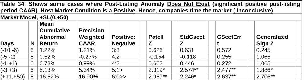
The starting set of hypotheses is when I test of whether the ―Post-Listing Anomaly‖ exists given different choices of benchmarks and estimation procedures. In doing so, the logic was if the host market was a positive and yet post-listing CAAR was a negative then the ―Post-Listing Anomaly Exists.‖ My view around that is, because I‘m using different benchmarks index returns as a proxy for the host market condition and the same benchmark index return is used in the estimation procedure to determine abnormal returns, therefore the results will be consistent, and I will be able to draw valid inferences from my tests.
H0: Post-listing anomaly exists regardless of benchmark types
HA: Post-listing anomaly does not exist regardless of benchmark types
The following hypotheses draws conclusions on the motives of companies to cross list, by relating host market condition to the post-listing returns or in other words the post-listing anomaly
H1A: Companies time the market
H1B: Companies do not time the market
H1B: Companies time or do not time the market (inconclusive)
The following hypotheses re-examine the relationship between host market condition, post-listing anomaly, and market timing when using different benchmarks and estimation procedures
H2B: Different benchmarks & Different estimation procedures produce different results.
It is important to note that those hypothesis will be tested simultaneously because they are inter-related, and for space considerations as well.
Research Method:
This paper examines returns using daily data, as Fama (1991, p.1607) notes, ―The cleanest evidence on market efficiency comes from event studies, especially event studies on daily returns.‖
Event studies seek to analyze the impact of a specified class of events on the prices of securities. The most widespread use of the event paper is in testing the Efficient Market Hypothesis (EMH). Showing demonstrated efficiency that the market response to an event takes place either before the event or very shortly after the event. Information is either expected or very quickly assimilated. The pioneering work on event study was done and Brown (1968) and Fama, Fisher, Jensen and Roll (1969). The methodologies used in these studies have become a standard technique for testing the EMH. Though several modifications have been made to the original methodologies, their basic structure has remained unaltered. The effect of the arrival of new information on a company‘s return may be interpreted as a change in the moments of the company‘s return distribution over the event period. With standard event paper methodology, the test is focused on the change in the mean of the company‘s return distribution
To discover the event impact I need a measure of abnormal return. But first I define daily returns as
Where is the daily security return at time , is the closing price of security at time , and is the closing price of security at time As was shown in Moustafa Fadl (2010) the variable‖ ‖ which is the domestic daily stock returns‖ was significant from Zero and that data daily returns are not normally distributed.
Since, the daily stock return for an individual security exhibits substantial departure from normality that is not observed with monthly data. The evidence generally suggests that distributions of daily returns are fat-tailed relative to a normal distribution {Fama (1976), p.21). Brown and Warner (1984) indicate that this also the case for excess returns based on daily data. However, this fact
need not necessarily bias hypothesis test toward type I error. The central limit theorem [ see Billingsley (1979,PP.308–319)] guarantees that when returns in the cross-section of securities are independent and identically distributed drawings from finite variance distributions, the distribution of the sample mean returns converges to normality as the number of securities increases. There is some evidence that the distribution of the cross–sectional daily mean return converges to a normal [Blattberg and Gonedes (1974)] when the return on a security and the return on the Market Index are each measured over a different trading interval Brown and Warner (1980, 1984) provide evidence that the t-test is an accurate test for the presence of abnormal performance despite the non-normality of the distribution of daily residuals Pamela P. Peterson (1989) reported that tests using daily returns are more powerful than those using monthly returns and the non-normality of stock returns has little impact upon properties of test statistics. Brown & Warner (1980) Daily returns have smaller standard deviations than do monthly returns. The use of daily data enables the research to take advantage of prior information about the specific day of the month on which the event took place
Implicit in the t-tests which are used to assess abnormal return are a number of strong assumptions: for example , in order for the test statistics to be distributed student–t , security returns must be normally distributed, if such assumption is not met , then the sampling distribution of test statistics assumed for the hypothesis tests could differ from the actual distributions, and false inferences could result if the distribution of the test statistic is miss-specified, then the null hypothesis, when true , could be rejected with some frequency other than that given buy the significance level of the test. Hence, I used non-parametric tests which make less restrictive assumptions than the t-test, those include: the Sign Test and a Wilcoxon Signed Rank Test [Kaplan and Roll 1972, Brown and Finn (1977)], and Collins (1979)].
……… (2)
Researchers have used a variety of models of the return generating process in lieu of the Market Model. They compute the abnormal returns on the basis of the assumed return generating process. After extensive testing of several models such as mean adjusted returns, market adjusted returns, market and risk adjusted returns, Brown and Warner (1980) conclude that when events are not clustered in time, the differences between the various methodologies are quite small. For the case where events are ―clustered,‖ the mean adjusted returns model is decidedly inferior.
Recent research model returns as drawn from a fat-tailed distribution with finite higher moments such as the distrbution, or as drawn as a mixture of distributions. The result is a fat-tailed unconditional distribution with a finite variance and higher moments, and since all moments are finite, the central limit theorem applies. Abnormal return is the actual ex-post return of the security over the event window minus the normal return of the company over the event period. The normal return is defined as the return that would be expected if the event did not take place. For each company and event date
I have
Where ) are the abnormal, actual, and normal returns, respectively, for time period . , is the conditioning information for normal performance model. I used the Market Model to model normal returns or expected returns. The Market Model assumes a stable linear relation between the market and the security returns.
Guidolin & Timmermann, (2005), identify three states that can broadly be interpreted as a high- volatility ‗bear‘ state with large, negative mean returns, a ‗normal‘ state with returns closer to their historical averages and a ‗bull‘ state with high mean returns on stocks and bonds. Specification tests that consider the full probability distribution of asset returns strongly reject single-state. Antonios Siganos et al (2006), the Momentum anomaly states that shares that performed the best (worse) over the previous three to twelve months continue to perform well (poorly) over the subsequent three to twelve months. Evidence suggests that strategy that buys previous winner shares and sells short
past loser stocks can generate abnormal profitability of approximately 1% per month (Jegadeesh and titman, 1993). Griffin et al. (2003) reported that Momentum profits tend to be stronger during down markets. Cooper et al. (2004) argued that Momentum profits are more pronounced following up markets. Antonios Siganos et al (2006) bull and bear markets are defined based on market return over various time horizons, and it is found that Momentum gains are more pronounced following down markets
The host market condition is represented by different proxies that correspond to the specific benchmarks I use for each analysis. I define the host market condition proxy, as the average DJIA index return is from day (0) to +50 days; Size- as the average portfolio returns from day (0 ) to +50 days that is formed on Size- ; BE/ME- as the average portfolio returns from day (0 ) to +50 days that is formed on BTM and Size—as the average portfolio returns from day (0 ) to +50 days that is formed on BTM and Size; Momentum— as the average portfolio returns from day (0 ) to +50 days that is formed on Momentum; Sentiment—the average portfolio returns from day (0 ) to +50 days that is formed on Sentiment index-; LTR- as the average portfolio returns from day (0 ) to +50 on LTR index ; STR- as the average portfolio returns from day (0 ) to +50 days that is formed on STR-.I define the host market condition indicator, as such, if the average index return after the listing date(0,+50) was a positive then the host market condition was a positive . Since I‘m using the Market Model to estimate normal return and I used the daily index returns as the proxy for the market portfolio ,then by definition the estimated normal return will reflect those host market conditions , by doing so then the estimated abnormal return should also reflect those host market conditions
There is evidence that the variance of stock returns increases for the days immediately around events.
Brown and Warner (1985) indicate that the failure to take into account non-synchronous trading in estimating Market Model coefficients does not result in misspecification. However, the correct specification of the model is consistent with the evidence presented by Scholes and Williams and Dimson (1979) that OLS estimates of β are biased. But, even when biases in β exist they do not necessarily imply misspecification in the model. By construction OLS residuals for a security sum to zero in estimation period so that a bias in the estimate of β is compensated for by a bias in α. With stationary, the event period returns for individual security can be shown to have a mean equal to zero unconditional on the market return. The return conditional on the market is biased for an individual security. However, no misspecification in an event study is implied if the average bias in conditional returns of the sample securities is zero; this occurs if securities are drawn from a representative range of trading frequencies or if there is none clustering of event dates. Moreover, there is no evidence that procedures other than OLS improve either the specification or the power of the tests. Although biases in β due to non-synchronous trading did not affect tests for abnormal performance, non-synchronous trading could also induce serial correlation in mean returns measures. For hypothesis test over intervals of more than a day, the failure to take into account autocorrelation in estimating the variance of cumulative mean returns could result in misspecification. Warner and Brown (1985) found that with a simple autocorrelation adjustment no dramatic changes occurred. Thus, the benefits from autocorrelation adjustments appear to be limited.
In order to address the criticism to the Market Model approach described above and to address the issues raised about the standard event study methodology I will use other estimation procedures that I will describe below
Market Model with Scholes Williams Beta Estimation: (Scholes and Williams, 1977) used a different way to estimate the beta:
. ………. (4)
Where is the OLS slope estimate from the
simple linear regression of on , is the
OLS estimate from the regression on ,
and is the estimated first–order autocorrelation of . As in OLS, the intercept estimator forces the estimated regression line through the sample mean:
. . . (5)
is the mean return of stock j over the estimation
period is the mean market return over the estimation period.
within the relevant inside-event window to which the observation belongs.
Giaccotto and Ali (1982) have shown that the standard tests to measure the effect of a specific event on security prices have to be adjusted to take into account the presence of heteroscedasticity. Akgiray (1989), Corhay et al, (1994) show that the empirical characteristics of return series can be described by Generalized Autoregressive Conditional Heteroscedasticity (GARCH) models, developed by Bollerslev (1986, 1987), which allow for non-linear inter-temporal dependence in the residual series. Bera, Bubnys and Park (1988) showed Market Model estimates under ARCH processes are more efficient and Diebold, Im and Lee (1988) observed that residuals obtained using the standard Market Model exhibit strong ARCH properties. The generalized autoregressive heteroscedasticity (GARCH) model, any large shock to a share price which causes an exceptionally high or low abnormal return on a particular day, also causes the variance of returns to be high on the following day, and to decay only slowly back to its long-run average ―unconditional‖ value. So the Market Model corrected for GARCH is
, where
. . . . .. . . . .. . . (6),
and
. . . (7), with
,
and , and
is the shock to returns on day of event , and is the time-varying variance of returns. The GARCH equation makes the variance on day to be conditional on the variance of the previous day ( and most recent squared shock
in a steady state, with the squared shock set to its expected value ( , and the variance
constant over time so that , the unconditional variance of event is
. . . . .. . . (8)
Even though GARCH models with conditional normal distribution allow unconditional error distribution to be leptokurtic, they might not fully explain the high level of kurtosis observed in the distribution of the returns series. Several leptokurtic
conditional distribution have been applied in the literature (Baillie and Bollerslev (1989) and Hsieh (1989); it is generally accepted that the distribution performs better. In conditional hetroskedastic models, the stability condition of the variance process requires that the sum of the estimated parameter, which measures the persistence of the volatility of firm, to be less than one. If this sum is equal to one, the process becomes an integrated GARCH or IGARCH (Engle and Bollerslev, 1986). Such integrated process implies the persistence of a forecast of the conditional variance over all future horizons and also an infinite variance of the unconditional distribution of . So I estimated the Market Model using E-GARCH where:
. . . . .. . . . .. . . (9),
Where
All parameters in both models are estimated using the maximum likelihood. I will report only Market Model estimated by GARCH unless there is a difference when using E-GARCH, in that case I will report both.
.
Market Adjusted Returns Model
MAR is computed by subtracting the observed return on the Market Index for day , from the rate of return of the common stock of the firm on day :
. . . . .. . . (10)
Once we make the adjustments then we follow the exam same procedure described in the Market Model to calculate the abnormal and cumulative abnormal returns.
4.1.4 Comparisons Period Mean Adjusted Returns
CP are computed by subtracting the arithmetic mean return of the common stock of the
firm computed over the estimation period, Once we make the adjustments then we follow the exam same procedure described in the Market Model to calculate the abnormal and cumulative abnormal returns
Hypotheses Testing Parametric Tests
assuming cross-sectional independence. Many published studies use the Patell test (Linn and McConnell, 1983; Schipper and Smith, 1986; and Haw, Pastena and Lilien, 1990).
The test statistic for the null hypothesis that is
. . ... . . . (11)
Under cross-sectional independence of and other conditions, follows the standard normal distribution under the null hypothesis. If abnormal returns are serially uncorrelated, the variance is the sum of the variances of daily abnormal returns:
Instead of using average standardized abnormal return the paper reports precision-weighted cumulative average abnormal return. The precision-weighted , as a weighted average of the original , preserves the portfolio interpretation that offers but average does not.
The Patell test statistics for abnormal returns cumulated over specific periods are not adjusted for serial dependence. Mikkleson and Partch (1988) perform such correction on collative returns. The serial dependence is not due to any presumed dependence in true Market Model error term, but occurs because all of the abnormal return estimators being cumulated are functions of the same estimators of the Market Model parameters. The derivation of the corrected standard error used by Mikkleson and Partch (1988) requires that the abnormal return be interpreted as forecast error.
If abnormal returns are serially correlated then following Mikkleson and Partch (1988), the corrected test statistic for the null hypothesis that
is
. . . . (12)
The corrected test accounts for the fact that within the window, the abnormal returns for each stock are serially correlated. Applications of the corrected test in addition to Mikkleson and Partch (1988) include Mais, Moore and Rogers (1989), Cowan, Nayar and Singh (1990), Mann and Sicherman (1991) and Lee (1992). The bias in the uncorrected test is small in event windows shorter than 60 days but serious in event windows longer than 100 days.
Cross-Sectional and Standardized Cross-Sectional Test: With standard event paper methodology, the test is focused only on the change in the mean of the company‘s return distribution: only the change in average returns is investigated. However, the change in the mean of the distribution may also be accompanied by a change in higher moments of the distribution. For example, on average, the arrival of new information may or may not have affect on a company‘s average return, but the company‘s average event-day release of information may increase the returns dispersion. Patell and Wolfson (1979), Kalay and Lowenstein (1985), Rosenstein and Wyatt (1990), Boehmer and Musumeci (1991) all describe a significant increase in return‘s variance around an event, and in some cases the variance increases to more than a three and a half times the variance on the estimation period ( Dann, 1981).
Cross-sectional tests are a standard part of almost every event paper. They are relevant even when the mean stock price effect of an event is zero. One reason that abnormal returns vary cross-sectionally is that the economic effect of the event differs by company. For such a situation, Sefcik and Thompson (1986) examine the statistical properties of cross-sectional regressions. They argue that accounting for cross-sectionally correlated abnormal returns and heteroscedasticity in the abnormal returns is potentially important for inferences.
When there is cross-sectional dependence , failure to make adjustments for it results in a systematic under estimation of the variance of mean returns implying too many rejections of the null hypothesis , both when it is true and when abnormal return is present beaver (1981) , and Dent and Collins(1981) . Collins and Dent (1984) propose a generalized least squares technique when the variance of each company‘s abnormal return estimator increases proportionally during the event period. Froot (1987) suggests a method of moment‘s estimator that allows for event-induced heteroscedasticity. Perhaps the simplest solution to the problem of event-induced heteroscedasticity is the one discussed by Boehmer, Musumeci and Poulsen (1991). The abnormal return estimates are first standardized by their estimated standard deviation (assuming no event-induced heteroscedasticity), based on the residual variance from the estimation period and the fact that they are prediction errors, as pointed out by Patell (1976). Then the standard deviation of these standardized variants SARs is calculated cross-sectionally in the event period and the significance of the estimate of the average standardized abnormal return ASARs (Average Standard Abnormal Returns) is tested using the cross-sectionally estimated standard deviation. In effect, this method assumes that the event-induced increase in variance is proportional for each company. Boehmer, Musumeci and Poulsen (1991) find in simulations that with this method the frequency of rejection of the null is essentially equal to the nominal size of the test when the null hypothesis of no abnormal performance is true. When the null is false, their method rejects the null more often than the other methods for which the true size of the test is equal to the nominal size. That is, their test is unbiased and more powerful than other well specified alternatives.
Boehmer, Musumeci and Poulsen (1991) introduce the standardized cross-section test and report its empirical properties. The test is the same as the Patell test except that there is a final empirical cross-sectional variance adjustment in place of the analytical variance of the total standardized prediction error, Sanders and Robins (1991). For day in the event period, the test statistic is
. . . .. . . (14)
Then the standardized cross-sectional test statistic for the null hypothesis that
is
. ……… (15)
Brown and Warner (1985) report that the cross-sectional test is well specified for event date variance but not very powerful, however Boehmer, Musumeci and Poulsen (1991) report that the standardized cross- sectional test is more powerful and equally well specified,
Crude Dependence Adjustments:
There is also a problem with time-series dependence. Under the joint hypothesis that returns are given by the Market Model with stationary parameters and that the market is informational efficient, Fama (1976), the disturbances in the Market Model, are independent across time. Neither the residuals nor the prediction errors from the Market Model are independent across time as assumed in many event studies. As Mikkleson and Partch (1988) and Mais, Moore and Rogers (1989) discuss, that regression residuals (and similarly prediction errors) are correlated since they are based on the same parameter estimates. To solve this problem the paper uses the crude dependence adjustments method
Brown and Warner (1980, 1985) used a procedure called ―crude dependence adjustments‖ where the standard error for this test is computed from the time-series of portfolio mean abnormal returns during the estimation period. Unlike the standardized abnormal return test, the time-series standard deviation test uses a single variance estimate for the entire portfolio. Therefore, the time-series standard deviation test does not take account of unequal return variances across securities. On the other hand it avoids the potential problem of cross-sectional correlation of security returns. The portfolio test statistic for day in event time is:
. (16)
The test statistic for is
4.2.4 Skewness–Adjusted Transformed Normal Test
The transformed normal test produced by Hall, (1992) is employed in this paper to correct for Skewness We first estimate the cross-sectional standard deviation and then calculate the Skeweness, so we arrive at
The Skewness adjusted transformed normal test statistic:
. …. (18)
Hypotheses Testing Non-Parametric Tests
Previous studies have shown that abnormal returns distributions show fat tails and are right Skeweness. Parametric tests reject too often when testing for positive abnormal performance and too seldom when testing for negative abnormal performance. When the assumption of normality of abnormal returns is violated, parametric tests are not well specified. Non-parametric tests are well specified and more powerful at detecting a false null hypothesis of no abnormal returns.
Generalized Sign Test
The Sign Test is a simple binomial test of whether the frequency of positive abnormal residuals equals 50%. The generalized test is a refined version of this test by allowing the null hypothesis to be different from 0.5. To implement this test, we first need to determine the proportion of stocks in the sample that should have non-negative abnormal returns under the null hypothesis of no abnormal performance. The value for the null is estimated as the average fraction of stocks with non-negative abnormal returns in the estimation period. If abnormal returns are independent across securities, under the null hypothesis the number of non-negative values of abnormal returns has a binomial distribution with parameter p. The alternative hypothesis, for any level of abnormal performance, is that the proportion is different than that. The advantage of the generalized Sign Test is that it takes into account the evidence of Skewness in security returns. The following statistic has an approximate unit normal distribution:
. ……… (19)
Where is the observed fraction of positive returns computed across stocks in one particular event, or the average fraction of companies with
non-negative abnormal returns for events occurring over multiple days
This test considers that both the sign and the magnitude of abnormal returns are important. For each window, I report the number of securities with positive and negative abnormal returns (cumulative abnormal returns as well) the null hypothesis for the generalized Sign Test is that the fraction of positive returns is the same as in the estimation period. The actual test uses the normal approximation of binomial distribution (Sanger and Peterson (1990)], Chen , Hu and Shieh (1991) Cowan (1992) report also that generalized Z test is well specified for event date variance increases and more powerful than the cross-sectional test. Cowan. (1992) the generalized Sign Test controls for the normal asymmetry of positive and negative abnormal returns in the estimation period
Scope of the Research
This paper aims at answering does the selection of different benchmarks, and different estimation procedures affect the sign, and the significance of the post-listing abnormal returns. As such, this paper is focused only on forming portfolios based on certain characteristics and using benchmarks that are appropriate for those characteristics, which I called the Characteristic Index based analysis. In addition, this paper was also focused on forming portfolios based on the Market Index and using different Market Index benchmarks that are suitable for such analysis, which I called the Market Index based analysis. Also, this paper used different estimation procedures to determine if that will change the sign and the significance of the post-listing abnormal returns, and to find the method that is a better fit when using daily returns data. Moreover, the paper objective is to show how the choice of the correct benchmark and estimation procedure will affect the interpretation of the post-listing abnormal returns. The paper provided a comprehensive analysis and comparison between the Characteristic index and the Market Index as well as comparisons between different estimation procedures.
Sample
companies who had their shares listed in their home market or on any other stock exchange except the U.S market before them cross-listed in the U.S. market. In addition, the sample did not include IPO companies, because the purpose is to examine the impact of cross-listing event on post-listing returns. See Table 1 below for a list of companies and their daily average returns along with the corresponding host Market Index returns (DJIA)
Source of Data: I collected the list of Non-US companies listing in U.S market along with the listing dates From NYSE and NASDAQ Fact book respectively, I then verified those companies through CRSP. Moreover, I checked World Scope Data Base and Thompson Reuters Data Base to verify the foreign country and foreign stock exchange as well. I collected pre-listing daily prices from Data Stream Data Base, and I collected post-listing daily prices from CRSP daily stock prices tape and verified it through Data Stream Data Base. I used the closing price of the stock at the each day and I matched the daily price with the daily price of the Market Index. The collection of daily stock prices and daily Market Index process will help determine daily stock return, and daily Market Index return respectively. By nature pre-listing return is foreign daily stock return, and it is calculated by change in prices without dividends. I have transformed daily foreign prices to US dollar currency at their respective dates using the exchange rates that were prevalent at that time and I verified that using Data Stream Data Base.
In order to obtain a U.S. listing, a foreign company must file a formal application with the U.S. exchange. It usually takes about four weeks for the NYSE and only a few days for the NADAQ to approve or reject the application. The submission of a formal application for the NYSE listing is announced in weekly bulletins published by each exchange on the first-day following the application. The first public announcement concerning an application for NASDAQ listing is made electronically through the NASDAQ terminals worldwide when the application is approved. Thus, the submission of the NASDAQ application itself is not formally announced. Unlike NYSE, NASDAQ does not require a confidential preliminary review of the eligibility. Once the application to NYSE or NASDAQ is approved, the company decides on the
date, in consultation with the exchange, when the company‘s stock will be actually listed.
For non-U.S. companies, the importance of a cross-listing announcement comes from its strong indication of the management‘s confidence in its company‘s global operations. Moreover, the cross-listing application acceptance carries another positive sign, this time by the foreign stocks exchange, regarding the company‘s ability to compete internationally by cross-listing abroad. Additionally, Lau at el. (1994) find that price reactions are most likely to happen on the first trading day and not on either the cross-listing application or acceptance dates. For unseasoned stocks listed in U.S. and then cross-listed abroad, Valero at el. (2008) analyzed the stocks‘ behavior around the listing day rather than the announcement dates due to difficulties in identifying the exact announcement dates. Out of 209 cross-listed stocks abroad they have in their full sample, they identify the exact cross-listing dates for only 46 stocks, finding significant positive average abnormal returns on the day before cross-listing and significant positive accumulative average abnormal return on the day of cross-listing. I will not examine the announcement effect because sometimes a company spokes person may indicate steps to cross list, then few months later there may be additional announcements of new steps or some negotiations being finalized. Therefore, it is difficult to consider the announcement date and hence the pre-announcement estimation period and event date will be continuously changing, so the event date will be the actual listing date