Multi-objective assembly line balancing using genetic algorithm Pages 863-872 Download PDF

(1)

* Corresponding author. Tel.: +98-9113762417. Fax: +98-1722233964 E-mail: [email protected] (S. Ayazi)

Contents lists available at GrowingScience

International Journal of Industrial Engineering Computations

homepage: www.GrowingScience.com/ijiec

Multi-objective assembly line balancing using genetic algorithm

Samad Ayazia*, Abdol Naser Hajizadehb, Mostafa Emrani Nooshabadic, Hamid reza Jalaiea and Yaghoob Mohammad moradid

a_{Department of Accounting and Management, Islamic Azad University, Aliabad Katool Branch, Aliabad Katool, Iran} b_{Department of Railway, Iran University of Science & Technology, Tehran, Iran}

c_{Department of Industrial Engineering, Iran University of Science & Technology, Tehran, Iran} d_{Department of Engineering, Islamic Azad University, Aliabad Katool Branch, Aliabad Katool, Iran} A R T I C L E I N F O A B S T R A C T

Article history:

Received 25 January 2011 Received in revised form April, 22, 2011 Accepted 24 April 2011 Available online 26 April 2011

One of the primary issues in line balancing problems is the uncertainty associated with the processing times. There are different reasons for having uncertain processing times such as task deterioration, failure in machines, etc. On the other hand, there are different objectives, such as cycle time, number of workstations in an assembly line balancing. In this paper, we present a multi-objective decision making assembly line balancing which minimizes different objectives such as cycle time and number of workstations. The resulted problem is formulated based on Lp-norm mixed integer programming and a meta-heuristic approach is also presented to solve the resulted model. The problem formulation is solved for some test examples and the results are discussed under different conditions.

Keywords:

Assembly line balancing Genetic Operators Multi-objective Genetic algorithm

1. Introduction

(2)

864

objective for a given cycle time by presenting a mathematical model. Gokcen et al. (2006) presented new procedures and a mathematical model on the single model assembly line balancing problem with parallel lines. Simaria and Vilarinho (2007) developed an ant colony optimization algorithm for two sided assembly line balancing problem and the primary goal was to minimize the number of work stations. Agpak and Gokcen (2005) presented a new approach on assembly line balancing problem. They developed a mathematical formulation to the balancing assembly line to minimize the number of work stations and resources. Bautista and Cano (2008) presented some procedures to minimize work over load in the mixed-model assembly lines. Peeters and Degraeve (2006) presented a new lower bound, namely the LP relaxation of an integer programming formulation based on Dantzig– Wolfe decomposition. In addition, they developed a branch and bound algorithm to solve the simple assembly line balancing (SALB) problem. Lapierre et al. (2006) developed a tabu search algorithm for balancing assembly lines. In the field of scheduling and balancing assembly lines, Tadeusz Sawik (2002) presented a monolithic and a hierarchical approach for assembly lines. The objective he considered was to determine an assignment of assembly tasks to stations and an assembly schedule for all products to complete the products in minimum time. Andre´s et al. (2008) considered the balancing and scheduling tasks in assembly lines, simultaneously. They added the sequence-dependent set up times to the SALB problem. They assumed that if a task assigned next to another task at the same workstation, the set up time should be added to compute the cycle time. They also presented a mathematical model along with some heuristic procedures. Toksari et al. (2008, 2010) studied scheduling and balancing assembly lines by considering the learning effect in the assembly lines. They showed that polynomial solutions can be obtained for both straight and U-shaped assembly line balancing with learning effect. Also Emrani Noshabadi et al. (2011) considered the simple assembly line balancing problem with additional scheduling issue based on the tasks deterioration element, they considered the single objective of number of workstations.

2. Problem description

2.1. Problem definition

Consider a line-balancing problem where there are N dependent tasks, which should be assigned and scheduled in workstations. These tasks have deterioration trait and deteriorate if there is a delay in their starting time. Tasks deteriorate while waiting to be processed. By the effect of task deterioration, task’s processing time increase if it is processed with delay. Thus, the processing time of each task depends on its starting time and the available time of that task. There is k undetermined work stations

1, ...2 R

s s s and the sequence of these stations in straight assembly lines is based on their number of indexes (i.e. s₁stands before s₂ and s₂stands before s₃and so on). Maximum number of work stations is equal to number of all tasks (every task in one separate work station) and the minimum number of workstations is equal to 1 (all tasks are in the one work station). We schedule and assign these tasks in stations by considering precedence relationships with objective function of minimizing the cycle time, number of stations and work load deviation which are considered for the first time simultaneously in this paper. For more details regarding to problem assumptions see (Emrani Noshabadi et al., 2011).

3. Mathematical formulation 3.1. Notation

N: The number of all tasks PS_k The processing time of station k

Z: Number of work stations T_k: The starting time of station k

k: k Z∈ =

{

1...Z_max

}

,It designate the work Coi: Completion time of task i j: It designates the position of job in the

sequence. j SE∈ =

{

1... ,L L N

}

= j

St : starting time of job that is assigned in sequence j, j∈SE={1,..., }L

i: ∈ =I {1,..., }N Designate the task. p_i: processing time of job i,

{ }

i

(3)

3.2. Formulation

Using the above notations, the mathematical model for simple straight assembly line balancing problem is developed as follows:

Decision variable

, ,

if task i in sequence j assign in station k other wise

1 0

i j k

x _{= ⎨}⎧

⎩

There are three objective functions of f1, f2 and f3 associated with the proposed model of this paper

and we use Lp-norm to find Pareto-optimal solutions as follows,

, * 3 * 3 3 * 2 * 2 2 * 1 * 1

1 1 2 3 ⎟⎟

⎠ ⎞ ⎜ ⎜ ⎝ ⎛ − + ⎟ ⎟ ⎠ ⎞ ⎜ ⎜ ⎝ ⎛ − + ⎟ ⎟ ⎠ ⎞ ⎜ ⎜ ⎝ ⎛ − = f f f w f f f w f f f w u (2)

where f1, f2 and f3 are CT, Z and W.D, respectively representing the cycle time, the number of work

stations and the work load deviation, respectively. The weights for each objective are shown with w, which are determined by decision maker.

1 1

( * )

L N

ijk i j i

Ct x p

= =

≥

∑∑

_{k m}_∈ _and

max

k Z≤ (3)

1

( )

Z

k k

k

y Ct q WD

Z

=

−

=

∑

k m∈ and k Z≤ max (4)

1 1 1 Z L ijk k j x = = =

∑∑

i I∈ , Z ≤Z_max (5)

1 1 1 Z N ijk k i x = = =

∑∑

_{j SE Z}_∈ _, _≤_Z_max (6)

1 1 0 L N ijk j i x = = ≥

∑ ∑

k m∈ k Z≤ _max (7)

1 1

( * )

N L

k ijk i

i j

q x p

= =

=

∑∑

max

k Z≤ (8)

(1 )

j ijk j i

C +M −x ≥St + p i I j SE k m∈ , ∈ , ∈ (9)

(1 )

j i ijk j

St + p +M −x ≥C i I j SE k m∈ , ∈ , ∈ (10)

1

j j

St

=

C

− j≥2, j SE∈ (11)

( )

( ) (S ( )

( ))

P i

=

a i

+

b i

×

t i

−

A V i

i I∈ (12)

(1 )

i ijk j

S + M − x ≥ St i I j SE k m∈ , ∈ , ∈ (13)

(1 )

j ijk i

St + M − x ≥ S i I j SE k m∈ , ∈ , ∈ (14)

1

(1 )

k ijk j

T +M −x ₋ ≥C i I j SE k m∈ , ∈ , ∈ ,k≥2 (15)

(1 )

j ijk k

St +M −x ≥T i I j SE k m∈ , ∈ , ∈ (16)

i g g

S ≥S + p i Jp g Ep∈ , ∈ _i (17)

Jp: Set of jobs that have predecessor b_i: The growth rate of the processing

i f j b

Np: Set of tasks that have no predecessor qk: Total processing time of station k

i

AV: The available time of task i a_i: Fixed part of the processing time of

j b

i

(4)

866

k ijk

y ≥x k m i I j SE∈ , ∈ , ∈ (18)

1 k k

y ≥ y+ k m∈ ,k Z≤ max−1 (19)

1 z k k Z y =

=

∑

₍₂₀₎

0

i

AV = i NP∈ (21)

{ }

max

i r

AV = C i Jp∈ , r Ep∈ _i (22)

i i i

CO = p +S i I∈ (23)

{ }

1, 0

k y = . 0 ) 1 ( , 0 ) ( ),

(j P i ≥ St =

C

k m∈ (24)

Eq. (2) shows the objective function, Eq. (3) describes the cycle time and Eq. (4) shows the workload deviation formulation. Eq. (5) and Eq. (6) state that each job and sequence occur once. Eq. (7) shows that some stations could be free of tasks (maximum number of stations is equal to number of all tasks). Eq. (9) and Eq. (10) describes the completion time of job in sequence j. Eq. (15) and Eq. (16) state that the starting time of station k is greater or equal to completion time of former station. Eq. (17) shows the precedence relations among tasks. Eq. (18) and Eq. (19) describe that task assigning process starts from early stations to last ones where there is no any vacant station between two busy stations. Eq. (20) shows the number of workstations. Eq. (21) and Eq. (22) describe the formulation of available time. Eq. (23) shows the formulation of task completion time.

4. Solution methodology 4.1. LP-metric

Lp-metric method is one of the prominent MCDM methods to address multi-objective problems with inconsistent objectives (Aryanezhad, et al., 2009; Mazdeh, et al., 2010). In this paper, a multi-objective integer programming model is developed to minimize the cycle time, workload and number of workstations. Mazdeh et al. (2010) recommended the LP-metric method to demonstrate the importance of two objectives in a bi-criteria parallel machines scheduling problem. Lp-norm has different forms of norm one, two and the norm one is the simplest form which helps us integrate different objectives. Suppose f1*, f*2 and f3* are the best values of three objective functions for our

proposed model. The LP-metric objective function can be constructed as follows:

, * 3 * 3 3 * 2 * 2 2 * 1 * 1

1 1 2 3 ⎟⎟

⎠ ⎞ ⎜ ⎜ ⎝ ⎛ − + ⎟ ⎟ ⎠ ⎞ ⎜ ⎜ ⎝ ⎛ − + ⎟ ⎟ ⎠ ⎞ ⎜ ⎜ ⎝ ⎛ − = f f f w f f f w f f f w u (10)

where w1, w2 and w3 are the weights of the objective functions determined by the decision maker. In

other word, the proposed model of this paper is first solved using each objective function, separately and then they are integrated using different weights with the utility function given in Eq. (10) into a single objective function and the problem is solved using different weights.

5. Genetic algorithm

Since the mathematical models does not give optimum solutions for large-scale problems in a reasonable amount of time, Meta-heuristic methods are exerted for these large problems to reach a near optimal solutions. Genetic algorithm (GA) raises a couple of important features. First it is a

stochastic algorithm; randomness as an essential role in genetic algorithms. Both selection and reproduction needs random procedures. A second very important point is that genetic algorithms always consider a population of solutions. GA can recombine various solutions to get better ones and it uses the benefits of assortment. A population base algorithm is also very amenable for

parallelization. The robustness of the GA methods is mentioned as something essential for the

(5)

There is no particular requirement on the problem before using GAs, so it can be applied to resolve any problem.

5.1. GA for multi objective SALB problem

This paper presented a GA for the simple straight assembly line balancing problem with deteriorating tasks. In the case of assembly line balancing Kim et al. (2009) developed a genetic algorithm for two-sided assembly line balancing called neighborhood GA (n-GA). They used straight forwardencoding scheme called group-number encoding. The individual they proposed was a string of length m (the

number of tasks), each element of which is an integer between 1 and n (the number of

mated-stations). Three main objective functions are considered in this paper as follows:

ct f₁=

min _{Minimizing the cycle time}

M f2=

min _{Minimizing the number of work stations}

wd f3=

min _{Minimizing the work load deviation}

Minimizing the work load deviation will balance the assembly line and minimize the idle times in the work stations. The general procedure of the GA that used in this paper is as follows:

Step 1: Initial population of chromosomes is generated in size p,

Step 2: Compute the fitness values of each chromosome,

Step 3: Choose a pair of chromosomes as parents by using the roulette wheels selecting method, generate offspring by doing crossover and then mutation with a probability of p_m(mutation probability).

Step 4: Insert the new population in to the new pool.

Step 5: If the stopping conditions are met, stop the searching process, select and decode the best chromosome and choose it as a the best solution. Otherwise, generate a new population and replace it with the former one and return to the step 3.

5.1.1. Representation

In this paper, each gene includes an integer number. Let n be the number of tasks in assembly line, each gene in chromosome includes an integer from 0 to n, also the number of all genomes in each chromosome which is against the zero is equal to number of all tasks which exists in the line. The position of gene in the chromosome, when a gene in a chromosome takes integer i not equals to zero, shows that task i is in which workstation and in what sequence is placed. As we can see from Fig.1,

the number of genes in each chromosome is _n2_.Each_n_{gene in the chromosome represents one}

workstationW_i. For an example, according to Fig. 1, task 1 is assigned to station 1 at the first sequence and task i is assigned to position n+1 and task k to n+5 shows that task i is assigned in station 2 before task k. Each chromosome should include integer numbers from 1 to n only for ones. Assigning integer i at the t’th gene shows that task i is assigned to station t 1

n

⎡ ⎤ + ⎢ ⎥

⎣ ⎦ . The maximum

(6)

868

1 2 …. n n+1 …. n+5 _n2 ₋1 _n2

1 0 … 0 i 0 k … 0 0

1

W W₂

Fig.1. An example of a chromosome

To prevent of creating vacant extra workstations between two occupied workstations, a checking process needs to be performed. In case the genomes from kn+1 to 2kn are zero, this means that no task is assigned

to this station and we can eliminate the genomes and shift all the previous genome by kn.

5.1.2. Initial population

Genetic algorithm starts by generating initial population of chromosomes. Every integer is assigned just for ones, next assigning 0 for the rest of the genes. This first population must offer a wide diversity of genetic materials. The gene pool should be as large as possible so that any solution of the search space can be engendered. For this aim the algorithm is done for several pool sizes and then results are checked. If all constrains hold for the generated chromosome it is added to the population and it is discarded, otherwise. For generating initial population, first the jobs with no predecessor are chosen for assigning randomly in chromosomes, next the chromosomes, which do not heed the precedence relations, are removed. After creating initial population, fitness value is computed for each chromosome. Fitness function is defined as follows:

1

fitness g

= . (25)

The g is defined as the following equation:

* * * * * *

1

1 1 1 2 2 2 3 3 3

( )

( ) / ( ) / ( ) /

Z

k k

Ct q

g w f f w CT f f w M f f

Z

=

−

=

∑

− + − + − . (26)

The first statement in Eq. (26) minimizes the work load deviation between work stations. CT and M

designate the cycle time and the number of workstations, respectively, q exhibits the total processing time of all tasks assigned to station k and w_irepresents the weighting values of objectives. With this definition of the fitness function, the objective of the algorithm is to maximize the fitness value. The

better fitness has bigger chance to enter the next population. The problem is tested by several

different values and the results are compared. The weights used in this paper is just to show the effectiveness of the weights in objective values, for using the algorithm in real situations decision maker can choose the weights, which are better for the problem.

5.1.3. Selection operation

(7)

selected as a parent. For example, if a chromosome number 1 has the fitness function of 4 and the chromosome number 2 has the fitness function of 6, then chromosome number 1 has the domain of [0,4] from the domain [0,T] and the chromosome 2 has the part of (4,10] from the domain [0,T].

5.1.4. Crossover operation

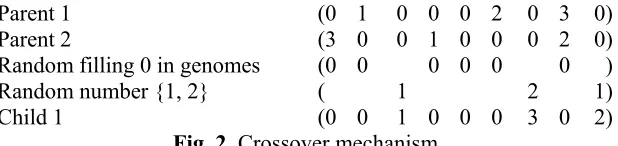
Crossover operator is applied to the mating pool with the hope that it creates offspring with a better fitness. In this paper a crossover technique, which is similar to precedence preservative crossover (PPX) crossover method is applied for the recombination. After selecting two parents for generating off springs, at first, an integer 0 value for the number of _n2₋_n_{items is assigned randomly in}

genomes of the chromosome. Next for the rest of the genomes we repeat a method which is similar to PPX crossover method. For this aim, integer random numbers from the set of {1, 2} are produced and they are assigned to the remained vacant genomes. The genomes except the ones which are labeled by 0. As we can observe from Fig. 2, the random integers of 1, 2 and 1 are assigned to vacant genomes. Integer number 1 indicates that the position of this genome in the chromosome must be filled by the first sequenced available task from parent 1. As we can observe, task number 1 is assigned in that position, which is selected from the first task from parent 1, and integer 2 shows that this position in the chromosome should be filled by the first sequenced task from parent 2 if it did not assigned already. In case it did, then the next sequenced task from parent 2 is selected. According to Fig 2, the next generated integer is 2 so task 3 is selected from the first available task from parent 2. Finally, the final randomly generated number is 1, so a task is selected from the next sequence and not the assigned task from parent 1 (task 2). More details for the procedure of PPX crossover method are available on the work by Sivanandam and Deepa (2008).

Parent 1 (0 1 0 0 0 2 0 3 0)

Parent 2 (3 0 0 1 0 0 0 2 0)

Random filling 0 in genomes (0 0 0 0 0 0 )

Random number {1, 2} ( 1 2 1)

Child 1 (0 0 1 0 0 0 3 0 2)

Fig. 2. Crossover mechanism

Therefore, the first child is produced by performing the method explained earlier and the next child is produced using the proposed rule. In this paper, we define an alternative way to produce the second child. First, the alternative method assigns number 1 for the same position of produced random number 2 in child 1 and number 2 for the position of produced random number 1 in child 1. Therefore, the positions of genomes with zero value are fixed. In this paper, the crossover method is performed in three types shown in Table 1 by considering these two procedures of producing child 2 and by naming the regular one as procedure 1 and the presented inversing one as procedure 2.

Table 1

Three types of used crossover methods

Type 1 Produce child 1, next produce child 2 through the first procedure Type 2 Produce child 1, next produce child 2 through the second procedure

Type 3 _{Apply type 1 and 2, then choose a pair of chromosomes from the set of}

{

_{p p ch ch}₁_, ₂_, ₁_, ₂

}

_by considering the fitness values

5.2.5. Mutation

The mutation occurs with the probability ofpm. Three kinds of mutation methods are considered in

(8)

870

randomly, which includes an integer between 1 to n and transfer it to the last sequence of former station or to the first sequence of the frontier station. The third one is to apply type 1 and 2 then choose a pair of chromosomes from the set of

{

p p ch ch1, 2, 1, 2

}

by considering the fitness values.

6. Computational results

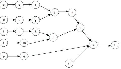
We first implement the proposed GA for three small examples and we compare the results with the optimal solutions. The proposed model has been solved by Lingo 8 mathematical software and the program has been coded by Java language and with PC 3.2 GHz CPU and 1 GB of RAM. Fig. 3 shows the example used in this paper with 20 tasks, which is the same as the example given by Kim et al. (2009).

Table 2 shows the precedence, times and other information of this example. In our implementation, crossover-probability is 0.3, mutation probability is 0.05 and population size is 100. The maximum number of iteration is 1000, the running time is limited to only ten seconds, the maximum variance of population size is one and the number of program run for each scenario is limited to 10. Table 3 also shows the results of our implementation.

Table 2

Fixed processing time and deterioration rate

Task A B C D E F G H I J K L M N O P Q R S T

Processing time _{3 3 6 8 3 4 7 3 3 8 3 3 6 3 5 9 10 3 4 7} Deterioration rate _{0.2 0.3 0.4 0.7 0.6 0.2 0.3 0.2 0.4 0.5 0.3 0.6 0.2 0.3 0.4 0.5 0.6 0.2 0.2 0.3}

Table 3

The Pareto-optimal results for different weights with g= Ct + W.D + M, Ct, M, W.D

size ₁_/₃

3 2 1=w =w =

w w1=0.6,w2=0.2,w3=0.2 w1=0.2,w2 =0.2,w3 =0.6

Solver Lingo GA Lingo GA Lingo GA

P4 8.44 8.44 8.22 8.22 8.44 8.44

Ct 6.4 6.4 6.2 6.2 6.4 6.4

M 2 2 2 2 2 2

W.D 0.04 0.04 0.2 0.2 0.04 0.04

P4 8.2, 8.2 7.385 7.385 7.385 7.385

Ct 6, 6 4.2 4.2 4.2 4.2

M 2, 2 3 3 3 3

W.D 0.2 0.2 0.185 0.185 0.185 0.185

P5 9.33 9.33 9.75 9.75 9.33 9.33

Ct 5.6 5.6 4.5 4.5 5.6 5.6

M 3 3 4 4 3 3

W.D 0.73 0.73 1.25 1.25 0.73 0.73

(9)

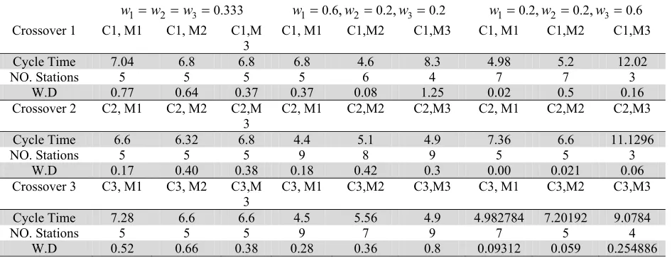
We have used the proposed GA method for another example from the literature where the input information of the problems with 12 tasks is presented in Table 4 and the Pareto-optimal solutions are summarized in Table 5 for different crossover mutation types. The first three rows of the table represent the results for crossover type 1, the second three rows present the results for crossover type 2 and the last three rows present the results for crossover type 3. As we can observe from Table 5, we get the best results for all three objectives when we use crossover number having equal weight set for all objective functions. For crossover type 2 and type 3 we may not find the best solutions for different weights under various mutation types.

Table 4

Fixed processing time and deterioration rate of the problem with 12 tasks

Task 1 2 3 4 5 6 7 8 9 10 11 12

Processing time 3 1 1 2 1 2 1 2 2 2 2 3

Deterioration

rate 0.4 0.3 0.3 0.1 0.1 0.5 0.3 0.1 0.2 0.2 0.1 0.5

Table 5

The results of GA for the example with 12 tasks and crossover type 1, 2, 3 and mutation types 1, 2 and 3

333 . 0

3

2

1=w =w =

w w₁=0.6,w₂=0.2,w₃ =0.2 w₁=0.2,w₂ =0.2,w₃=0.6 Crossover 1 C1, M1 C1, M2 C1,M

3 C1, M1 C1,M2 C1,M3 C1, M1 C1,M2 C1,M3 Cycle Time 7.04 6.8 6.8 6.8 4.6 8.3 4.98 5.2 12.02

NO. Stations 5 5 5 5 6 4 7 7 3

W.D 0.77 0.64 0.37 0.37 0.08 1.25 0.02 0.5 0.16 Crossover 2 C2, M1 C2, M2 C2,M

NO. Stations 5 5 5 9 8 9 5 5 3

W.D 0.17 0.40 0.38 0.18 0.42 0.3 0.00 0.021 0.06 Crossover 3 C3, M1 C3, M2 C3,M

NO. Stations 5 5 5 9 7 9 7 5 4

W.D 0.52 0.66 0.38 0.28 0.36 0.8 0.09312 0.059 0.254886

7. Conclusion

In this paper, simple straight assembly line balancing problem with deteriorating tasks have been considered. By existence of deteriorating tasks in assembly lines, the problem of assigning tasks to the workstations changes to scheduling and assigning tasks to the workstations. A mathematical model based on 0-1 integer programming model has been developed with the objective functions of minimizing the cycle time, number of work stations and work load deviation. Since these cases of problems fall in to class of NP-hard, mathematical model cannot be applied for large-scale problems. Therefore, we have proposed a genetic algorithm where three kinds of crossover and mutation methods are used. The implementation of the proposed model has been used for some well-known benchmark problems and the results have been discussed.

References

Andre´s, C, Miralles, C., & Pastor, R. (2008). Balancing and scheduling tasks in assembly lineswith sequence-dependent setup times. European Journal of Operational Research, 187, 1212–1223. Agpak, K., & Gokcen, H. (2005). Assembly line balancing: Two resource constrained cases.

International Journal of Production Economics, 96, 129–140.

Aryanezhad, M.B., Kheirkhah, A.S., Deljoo, V., & Mirzapour Al-e-hashem, S.M.J.(2009). Designing

(10)

872

Manufacturing Technology, 41, 193-199.

Aryanezhad, M.B., Jabbarzadeh, A., & Zareei, A., (2009). Combination of genetic algorithm and

LP-metric to solve single machine bi-criteria scheduling problem. Proceedings of the 2009 IEEE

IEEM, 1915-1919.

Bautista, J., & Cano, J. (2008). Minimizing work overload in mixed-model assembly lines.

International Journal of Production Economics, 112, 177–191.

Browne, S., & Yechiali, U. (1990). Scheduling deteriorating jobs on a single processor. Operations Research, 38, 495–501.

Chang, C.T., (2007). Binary fuzzy goal programming. European Journal of Operational

Research,180 (1), 29–37.

Emrani Noushabadi, M., Bahalke, U., Dolatkhahi, K., Dolatkhahi, S.,& Makui, A. (2011). Simple assembly line balancing problem under task deterioration. International Journal of Industrial Engineering Computations, 2(3), 583-592.

Fleszar, K., & Hindi, K. S. (2003). An enumerative heuristic and reduction methods for the assembly line balancing problem. European Journal of Operational Research, 145, 606–620.

Gokcen, H., Agpak, K., & Benzer, R. (2006). Balancing of parallel assembly lines. International Journal of Production Economics, 103, 600-609.

Jin, M., & Wu, S. D. (2002). A new heuristic method for mixed model assembly line balancing problem. Computers & Industrial Engineering. 44, 159–169.

Kara,Y., Paksoy, T, & Chang, C-T. (2009). Binary fuzzy goal programming approach to single model

straight and U-shaped assembly line balancing. European Journal of Operational Research,

195(2), 335-347.

Kim, Y. K., Song, W.S., & Kim, J. H., (2009). A mathematical model and a genetic algorithm for two-sided assembly line balancing. Computers & Operations Research, 36, 853 – 865.

Lapierre, S. D., Ruiz, A., & Soriano, P. (2006). Balancing assembly lines with tabu search. European Journal of Operational Research, 168, 826–837.

Mahdavi Mazdeh, M., Zaerpour, F., Zareei, A., & Hajinezhad, A., (2010). Parallel machines scheduling to minimize job tardiness and machine deteriorating cost with deteriorating jobs.

Applied Mathematical Modelling, 34, 1498–1510.

Ozcan, U., & Toklu, B. (2009). Multiple-criteria decision-making in two-sided assembly line balancing: A goal programming and a fuzzy goal programming models. Computers & Operations Research, 36, 1955-1965.

Peeters, M., & Degraeve, Z. (2006). An linear programming based lower bound for the simple assembly line balancing problem. European Journal of Operational Research. 168, 716–731. Sawik, T. (2002). Monolithic vs hierarchical balancing and scheduling of a flexible assembly line.

European Journal of Operational Research, 143, 115–124.

Scholl, A., Becker, C. (2006). State-of-the-art exact and heuristic solution procedures for simple assembly line balancing. European Journal of Operational Research, 168. 666–693.

Shahanaghi, K., Yolmeh, A. M., Bahalke. U. (2010). Scheduling and balancing assembly lines with the task deterioration effect". Proc. IMechE Part B: J. Engineering Manufacture, 224(7), 1145-1153.

Simaria, A. S., & Vilarinho. P. M. (2009). 2-ANTBAL: An ant colony optimisation algorithm for balancing two-sided assembly lines. Computers & Industrial Engineering, 56, 489-506.

Sivanandam, S. N. & Deepa, S. N. (2008). Introduction to genetic algorithms, 47–54 (Springer, Berlin/ Heidelberg/New York)

Toksarı, M. D., Selçuk, K. I, Güner, E., & Baykoç, O. F. (2010). Assembly line balancing problem with deterioration tasks and learning effect. Expert Systems with Applications. 37(2), 1223–1228. Toksarı, M. D., Selçuk, K. I, Güner, E., & Baykoç, O. F. (2008). Simple and U-type assembly line