__________
* Corresponding author
website: https://eoge.ut.ac.ir
Numerical determination of the geodesic curves: the solution of a two-point
boundary value problem
Mohammad Reza Seif 1*, Emad Ghalenoei2
1 Department of Surveying Engineering, Arak University of Technology, Arak, Iran 2 Department of Geomatics Engineering, University of Calgary, Calgary, Alberta, Canada
Article history:
Received: 20 October 2017, Received in revised form: 20 February 2018, Accepted: 25 March 2018 ABSTRACT
In this paper, we suggest a simple iterative method to find the geodesic path on a surface parameterized by orthogonal curvilinear system between two given points based on solving Boundary Value Problem. In this supposed method, an iterative algorithm is used for finding the sufficient initial values as the destination point agree with the boundary conditions. Geodesic determination between two given points is formulated for a general surface, and specially tested for reference ellipsoid which has many applications in geosciences and geodesy. Accuracy of the method is independent on the distant between two points on the surface. Moreover, it can be used in aviation and sailings for finding the shortest path between start and destination points.
S
KEYWORDS
Geodesic, geodetic computation
Boundary Value Problem Reference ellipsoid
1. Introduction
The problem of determining geodesic curve, shortest path between two points on a surface, has attracted much attention of many scientists in different fields in the recent years. It is due to many important classic and modern applications of geodesics, containing medical imaging, robotic movement, satellite orbits, positioning problem in geometrical geodesy, industrial application, garment design and etc. Geodesics arise in shoe industry for garment design. Given a model and size, the characteristic curve called girth is usually fixed, and preferably should be a
reasons (
geodesic for manufacturing Sanchez-Reyesa & Doradob, 2008; Azariadis & Aspragathos, 2001). A satellite's orbit around the attracting body of revolution on a plane orthogonal to the axis of rotation (z-axis) is a geodesic curve (Ghafari, 1970). Geodesics could be used for optimal trajectory planning in robotic applications (Zhange & Zhou, 2007; Zhang et al., 2010). The shortest path has some applications in tubular structures extraction
(
in 3D medical images Deschamps & cohen, 2001). analysis in image
introduced Geodesic distance was
(Lantuéjoul & Beucher, 1980) and applied by other scientists in the field of image processing (Kimmel, 1997; Lindeberg, 1994). It is also used in computer vision for object segmentation (Caselles et al., 1997; Cohen & Kimmel, 1997; Kimmel et al., 2000).
72 In general, the approaches for geodesic curve
determination can be divided into the analytical and numerical methods (Kasap et al., 2005). The analytical approaches; represented by Carmo (1976) are more complex and cannot be used in general case. Nevertheless, the numerical approaches; represented by Patrikalakis & Ko (2003) are classified as initial-value problem (IVP), four boundary conditions are given at one point, and the boundary-value problem (BVP), four boundary conditions are specified at two distinct points. The boundary value problem in geodesics could be solved by an easy but unstable method (shooting method) which is based on a finite difference approximation and more complex but stable method (relaxation method) which uses Newton method (Patrikalakis & Ko, 2003).
In this paper, we introduce a new method for finding the geodesic path between two given points i.e., the distance and azimuth on an orthogonal curvilinear surface, in particular the geodesic path on the rotational ellipsoid, using a simple and stable approach in the BVP mode. This approach uses iterative algorithm for adjusting the initial values in a way that the curve passes through the destination point.
2. Formulation of a geodesic curve
A surface represented by two independent curvilinear parameters (𝑢, 𝑣) is equivalent to a surface in a 3D Cartesian space. Therefore, each point on an arbitrary surface could be expressed by the two independent curvilinear parameters. The position vector in the Cartesian orthogonal system (𝑋1, 𝑋2, 𝑋3 ) is a function of curvilinear parameters as follow:
(1)
1
2
3
( , )
( , )
( , )
( , )
X u v
R u v
X u v
X u v
The curvilinear parameters are state as functions of an independent parameter
t
. Any arbitrary curve 𝛼(𝑡) on the surface can be represented as:(2)
( )
t
R u t v t
( ( ), ( ))
)
(
t
is a geodesic curve if and only if,u
(
t
)
andv
(
t
)
satisfy the following equations (Lipschutz, 1969):
(3)
2
1 2 1 1 2
11 12 22
2 2
2 2 2 2 2
11 12 22
2
(
)
2
(
)(
)
(
)
0
(
)
2
(
)(
)
(
)
0
d u
du
du dv
dv
dt
dt
dt
dt
dt
d v
du
du dv
dv
dt
dt
dt
dt
dt
where
ijkare the Christoffel symbols defined as (Patrikalakis & Ko, 2003):(4)
1
11 2
2
11 2
1
12 2
2
12 2
1
22 2
2
22 2
2
2(
)
2
2(
)
2(
)
2(
)
2
2(
)
2
2(
)
u u v
u v u
v u
u v
v u v
v v u
GE
FF
FE
EG
F
EF
EE
FE
EG
F
GE
FG
EG
F
EG
FE
EG
F
GF
GG
FG
EG
F
EG
FF
FG
EG
F
where
E
,F
, andG
are the coefficient of first fundamental form of the surface.(5)
, ,
R R R R R R
E F G
If
u
(
t
)
andv
(
t
)
are orthogonal,F
and their derivatives will be zeros. Then, the geodesic equations will have a simpler form:(6)
2 2
2 2
0
2
2
2
0
2
2
2
u v u
v u v
E
E
G
u
u
u v
v
E
E
E
E
G
G
v
u
u v
v
G
G
G
We have two second-order differential equations or equally four first-order differential equations. It can be achieved by defining the state vector
s
(
t
)
as:(7)
( )
( )
( )
( )
( )
u t
v t
s t
u t
v t
where (𝑢′(𝑡), 𝑣′(𝑡)) are the first order derivatives of the (𝑢, 𝑣) with respect to the independent variable 𝑡. The geodesic curve second-order differential equations (Eq. 6) are recast into the classical form of an initial value problem: (8)
o o
( )
( , ( ))
( )
s t
f
t s t
s t
s
where
s
o contains position of the origin(
u
o,
v
o)
and its first-order derivative or the so-called velocity at the origin)
,
72 methods i.e., numerical integrators. Moreover, velocity at
the origin is directly inestimable due to the nonlinearity of the system equations (
f
). The problem should be solved using an iterative scheme. The solution process is stared with an initial guess of velocity at the origin(
u
o0
,
v
o0
)
.Solving Eq. (8) with this initial guess yields a geodesic curve which might not passes through the destination point
)
,
(
u
fv
f . The initial value should be iteratively improved in a way that the resulting geodesic curve passes through the destination point. Taking this idea into account, the given initial state vector is assumed as an approximate value and the correction vectord
s
ˆ
in the following form is sought: (9)
o o o o o0
0
ˆ
ˆ
v
u
s
s
d
s
s
It shows that the correction vector only contains correction to the initial velocity.
Numerically, the problem can be expressed as an optimization problem. The aim is to find the correction to the initial velocity in a way that the deviation of the geodesic curve at the destination with respect to the given position is minimized. Theoretically, the deviation should be zero but it can be a very small negligible number from the computational point of view. In mathematical notation it reads: (10) f o f f o f f 2 2 f f f
ˆ
( ,
)
ˆ
( ,
)
u
u t s
u
v
v t s
v
u
v
Zero
where
(
u
f,
v
f)
are the differences between the given and the estimated position of the destination point. Assume the sought-after correction is small enough such that the linearization yields accurate approximation:(11)
o o0 o o o
o o0 o o o
f f f f
f f
ˆ
( ,
)
( ,
)
[
( ),
ˆ
( )]
ˆ
ˆ
( ,
)
( ,
)
,
u t s
u t s
u s
v s
u
v t s
v t s
u v
v
Inserting the linearized form into Eq. (10) yields:
(12)
o
o o f of f
o
f o o f f o
2 2 f f ˆ ˆ [ ( ), ( )] ( , ) , ( , ) f f
u s v s u u t s
u u
v
v u v v v t s
u v Zero
or equivalently, (13) o o u
d A d
v d Zero
where d is the misfit vector and the design matrix and the misclosure vector are denoted by 𝐴 and dl respectively. If the misfit vector will be zeros, applying the iterative method yields: (14) 1 o o
u
A d
v
Then, (15) 1 oo f f
o f f o
( ,
)
( ,
)
u
u
u t s
A
v
v
v t s
Eq. (15) can be rewritten in more detail as follows:
(16)
f o ( 1) 1
o o f
o ( ) o ( 1) f
f o ( 1)
,
,
n
n n
n
u t s
u
u
u
A
v
v
v
v t s
where (17) o o o ( 1)o( 1) o( 1) n n n
u
v
s
u
v
Computation procedure will be complete if the design matrix is calculated. The design matrix
A
is expressed as a product of partial derivative using the chain rule as:(18)
o o
o o
o o 1 2 1 o
1 2 1 o o o
ˆ
ˆ
[
( ),
( )]
,
ˆ
ˆ
[
( ),
( )]
,
f ff f n
n n
u s
v s
A
u v
u s
v s
s
s
s
s
s
s
s
s
u v
72 (19)
o o
1 2 1
2 1 1 o
ˆ ˆ [ ( ), ( )] ( , ) 0 0 0 0 ( , ) ( , ) 1 0 0 1 f f n n n
u s v s
A t t
s
t t t t
where (20)
1 o 1 2 2 1 1 o
(
t
n, )
t
(
t
n,
t
n)
( , ) ( , )
t t
t t
The transition matrix in numerical determination of geodesic curve is obtained by:
(21)
0 0 0 0
0 0 0 0
0 0
0 0 0 0
0 0 0 0
( ) ( ) ( ) ( ) ( ) ( ) ( ) ( ) ( ) , ( ) ( ) ( ) ( ) ( ) ( ) ( ) ( ) ( )
u t u t u t u t
u v u v
v t v t v t v t
u v u v
s t t t
u t u t u t u t s t
u v u v
v t v t v t v t
u v u v
Eq. (21) represents the general form of the transition matrix for numerical computation of geodesic curve on an arbitrary two-dimensional surface. To deriveΦ(𝑡, 𝑡0), one can use the Taylor expansion of the state vector in terms of the initial state. The expansion up to the second-order gives:
(22)
2
0 0 0
2
0 0 0
1
( )
( )
2
1
( )
( )
2
u t
u t
u dt
u dt
v t
v t
v dt
v dt
and (23) 0 0 0 0( )
( )
u t
u
u dt
v t
v
v dt
Both the position and velocity vectors are written in terms of the initial position and velocity vectors. Entries of the transition matrix are derived as follow:
(24)
02 2 2 2
0 0 0 0
0 0 0 0
2 2 2 2
0 0 0 0
0 0 0 0
0 0 0 0
0 0 0 0
1 0 0
0 1 0
,
0 0 1 0
0 0 0 1
( ) ( ) ( ) ( )
2 2 2 2
( ) ( ) ( ) ( )
2 2 2 2
( ) ( ) ( ) (
dt dt t t
u dt u dt u dt u dt
u v u v
v dt v dt v dt v dt
u v u v
u u u u
dt dt dt
u v u v
0 0 0 0
0 0 0 0
)
( ) ( ) ( ) ( )
dt
v v v v
dt dt dt dt
u v u v
Eq. (24) could be constricted in a new form:
(25)
02
0 0 0 0
2
0 0 0 0
0 0 0 0
0 0 0 0
1 0 0
0 1 0
,
0 0 1 0
0 0 0 1
0 2 0 2 0 0 dt dt t t dt
u u u u
u v u v
dt
v v v v
dt u v u v
dt
At final, we have
(26)
0 0 0 0 2 21 0 0
0 1 0
,
0 0 1 0
0 0 0 1
0 2 0 2 0 0 u v s dt dt t t dt dt dt dt
The term needed for computing transition matrix is Jacobian matrix 00
0 v u s
. More detail on the computation of the partial derivatives appeared in Eqs. (43) and (44) are given in Appendix 1. It should be mentioned that the Eq. (22) are used for determination of a geodesic curve in terms of dynamic process and concept of the state transition matrix. Eq. (6) can also be solved using ODE routines e.g. ODE113 in MATLAB, with error control of about 10-14 and03 3. Case Study: Geodesic curve on the rotational
Ellipsoid surface
A reference ellipsoid, an ellipsoid of rotation, is a suitable approximation of the shape of the Earth (Vanichek & krawinsky, 1986). Reference ellipsoid is a rotational one that formulated using two the size and shape parameters, i.e., semi-major axis and the eccentricity( , )a e of the ellipsoid. The geometry of ellipsoid is fully explained using the size and shape parameters. Therefore, all the geometrical computation (point positioning, area and volume calculation and etc.) is formulated using the size and shape parameters. The position vector of a point located on the surface of the reference ellipsoid in terms of the curvilinear coordinates (the geodetic latitude 𝜑 and geodetic longitude 𝜆 ) is expressed as (Jekeli, 2006):
(27)
2
( ) cos( ) cos( )
( , )
( ) cos( )sin( )
( ) 1
sin( )
N
R
N
N
e
1/ 22 2
( )
1 sin ( )
a N e
where N( )
is the prime vertical radius of curvature. Thecoefficients of the first fundamental form of the ellipsoid required for the geodesic equations are:
(28)
2
2 2
0
cos ( )
E
M
F
G
N
where M( )
is the meridian radius of curvature(Krakiwsky & Thomson, 1978):
(29)
2 3/ 2 2 2 1 ( )1 sin ( )
a e M e
By substituting
E
andG
of ellipsoid surface into Eq. (6) and after some manipulation, the geodesic differential equations for ellipsoid surface have final form:(30) 2 2 2 2 2 2 2 2
3
sin(2 )
sin(2 )
2 1
sin ( )
2
1
2
tan( )
1
sin ( )
e
e
e
e
The transition matrix needed for geodesic determination is derived as follow:
(31)
0 00
2
2 0
0
1
0
0
2
0
1
0
,
0
0
0
1
0
2
0
0
0
0
1
0
sdt
dt
dt
dt
t t
dt
dt
where Jacobian matrix components are:
(32)
2 2 2 2
2 2 2 2 2 2 2 2 2
2 cos(2 ) 1 sin( ) sin(2 ) 3
2 1 sin( )
cos(2 ) 0
sin(2 ) 3
1 sin( ) sin(2 ) e e e e e e And (33)
22 2 2 2
2 2 2 2 2 2 2 2 2 2(1 )
(1 tan( ) ) 1 sin( ) sin(2 ) tan( ) 1 sin( )
0 1
2 tan( )
1 sin( ) 1
2 tan( )
1 sin( )
e e e e e e e e
As shown, we need an initial value for the first derivatives of the curvilinear coordinates( ,
)at the start point. The initial value is calculated using the coordinates of the start and destination points based on a spherical approximation of the ellipsoid. Based on the spherical approximation, the azimuth and the length of geodesic curve are (Harris and Stocker, 1998):(34)
1
1 2
1 2 2 1
cos (sin( ) sin( ) cos( ) cos( ) cos( ))
1 2 2 1
1
cos( )sin( )
sin ( )
sin( )
Az
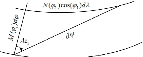
03 decomposed into the orthogonal latitudinal and longitudinal
elements as:
Figure 1. Line elements of curve on surface of the Earth
(35)
1 1 1
1 1
( ) cos( ) sin( )
( ) cos( )
N d d Az
M d d Az
where
(36)
0
lim
t
d
t
In this equation
t
is an independent parameter, it could be considered as the time needed for traveling a virtual moving particle from the start point to the destination point on the ellipsoid. The computation is not highly dependent tot
, but it should be considered small enough in such a way that the nonlinearity error can be ignored. d
andd
in the start point is the initial values for
1
and
1
when0
or equivalently
t
0
. Then, initial values for unknown parameters are:(37)
10 1
1
10 1
1 1
cos(
)
( )
sin(
)
( ) cos( )
d
Az
M
d
Az
N
The geodesic curve on the ellipsoid could be determined by applying the algorithm described in pervious section. Having the geodesic curve as a set mesh points with any arbitrary density, the differential element of the length and azimuth of a differential element on the geodesic curve is computed by:
(38)
2 2 2 2 2
cos ( )
d
N
d M d
(39)
1
cos( )
tan
N
d
Az
Md
Geodesics computed using this approach is represented in the next section.
4. Results and discussion
For the accuracy evaluation of the geodesic determined by Eq. (22), the length of geodesic curve derived from the proposed formulation is compared with that of the directly computed by solving differential equation. The evaluation is carried out for the following cases:
Case 1) Two points on a single meridian The length of geodesic curve 𝜓 is determined as:
(40) 2
1
2
1
2
( ) cos ( )
2 2 2( )
2d
N
d
M
d
Since
d
0
,
the Eq. (33) takes the following simpleform:
(41) 2
1
( )
M
d
In addition to approximate closed form relation represented for solving this integral (Krakiwsky & Thomson, 1978), it could be accurately solved using computing routines e.g. ODE113 in MATLAB. In Table 1, the solution of Eq. (41) is compared by that of the Eq. (22). The comparison is carried out for the pole-to-pole meridian arc length. The efficiency of the method represented for geodesic curve determination is tested on the surface of ellipsoid WGS84 (World Geodetic Datum 1984). A sub-millimeter level of accuracy in the computed geodesic curve length is considered for the maximum error tolerance. It is equal to 0.00001" in longitudinal and latitudinal differences, i.e., the maximum size of misfit vector at the end point. The error of each iteration in case pole-to-pole geodesic determination is represented in Table 2.
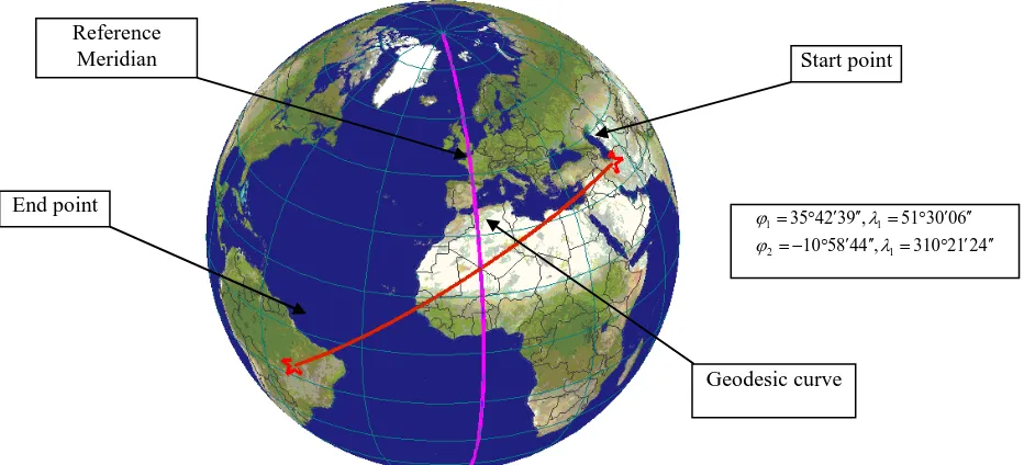
Case 2) Two points in arbitrary locations
Two arbitrary points are located in northern and southern hemisphere, see Figure 2.
Case 3) A nearly trans-polar geodesic curve
07 Table 1. Comparison of the pole-to-pole meridian arc length error
𝝍(𝐤𝐦) Error
(mm)
Number of iteration
Computation Time (sec)
start point destination point
( )
(
)
( )
(
)
20003931.458625 1.001 3 3.001 -90 0 90 0
Table 2. The error of each iteration in case pole-to-pole geodesic determination Iteration Error (m) Error (rad)
1 98642.60756 0.01546574
2 10.02431927 1.57E-06
3 0.001001454 1.57E-10
4 4.82E-07 7.55E-14
It should be mentioned here that the formulation given for numerical determination of geodesic curve on a sphere and the rotational ellipsoid is singular for the antipodes. Case 4) Geodesic between the points with equal latitude
A more illustrative example of geodesic curve is the shortest pass between two points on the rotational ellipsoid
with equal latitude. In the case of sphere the connecting parallel is the geodesic. However, it is different for the ellipsoid. Two arbitrarily selected points on a parallel are depicted in Figure 4. As shown, the geodesic curve tends towards the pole to minimize the arc length between the points.
Figure 2. The geodesic curve on the ellipsoid for the plotted points:
1 1
2 1
35 42 39 , 51 30 06
10 58 44 , 310 21 24
Start point Reference
Meridian
End point
4 2 1 2 310 , 4 4 8 5 10
6 0 0 3 1 5 , 9 3 2 4 5 3
1 2
1 1
00 Figure 3. A nearly transpolar geodesic curve on the
ellipsoid 1 1
2 1
30 , 115 55 , 290
Figure 4. The geodesic curve along the parallel on the ellipsoid
1 1
2 1
30 , 30 30 , 90
5. Conclusion and recommendations
In this paper, a new approach is proposed for numerical solution of the geodesic curve determination boundary value problem. It is formulated for any arbitrary surface in general and the Earth’s reference ellipsoid i.e., the rotational ellipsoid in particular. The efficiency of this approach in tested in few examples for the pair of points placed on the surface of the Earth. The new approach can be used for reformulation of geometrical computation in Geosciences and Geodesy applications.
It should be mentioned here that the formulation given for numerical determination of geodesic curve on a sphere and the rotational ellipsoid is singular for the antipodes. More investigation is required for removing formulation singularity in the trans-polar geodesic curve.
Reference
03 Baeschlin, C. F. (1948). Lehrbuch der Geodasie. Zurich,
Orell Fussli, 1948.
Bermejo-Solera, M., & Otero, J. (2010). Global optimization of the Gauss conformal mappings of an ellipsoid to a sphere. Journal of Geodesy, 84(8), 481-489.
Bessel FW (1825) Über die Berechnung der geographischen Längen und Breiten aus geodätischen Vermessungen. Astron Nachr 4(86):241–254. [Translated into English by Karney CFF and Deakin REas The calculation of longitude and latitude from geodesic measurements. Astron Nachr 331(8):852–861 (2010)]
Caselles, V., Kimmel, R., & Sapiro, G. (1997). Geodesic active contours. International journal of computer vision, 22(1), 61-79.
Cohen, L. D., & Kimmel, R. (1997). Global minimum for active contour models: A minimal path approach. International journal of computer vision, 24(1), 57-78. Deschamps, T., & Cohen, L. D. (2001). Fast extraction of
minimal paths in 3D images and applications to virtual endoscopy1. Medical image analysis, 5(4), 281-299. Do Carmo, M. P. (2016). Differential Geometry of Curves
and Surfaces: Revised and Updated Second Edition. Courier Dover Publications.
Ghaffari, A. (1971). On the integrability cases of the equation of motion for a satellite in an axially symmetric gravitational field. Celestial mechanics, 4(1), 49-53.
Grafarend, E. W., & Syffus, R. (1995). The oblique azimuthal projection of geodesic type for the biaxial ellipsoid: Riemann polar and normal coordinates. Journal of Geodesy, 70(1-2), 13-37.
Jekeli, C. (2006). Geometric reference systems in geodesy. Division of Geodesy and Geospatial Science, School of Earth Sciences, Ohio State University, 25.
Heitz, S. (1988). Coordinates in geodesy. Berlin; New York: Springer-Verlag, c1988.
Harris, J. W., & Stöcker, H. (1998). Handbook of mathematics and computational science. Springer Science & Business Media.
Karney, C. F. (2013). Algorithms for geodesics. Journal of Geodesy, 87(1), 43-55.
Kasap, E., Yapici, M., & Akyildiz, F. T. (2005). A numerical study for computation of geodesic curves. Applied Mathematics and Computation, 171(2), 1206-1213.
Kimmel, R. (1997). Intrinsic scale space for images on surfaces: The geodesic curvature flow. Graphical models and image processing, 59(5), 365-372.
Kimmel, R., Malladi, R., & Sochen, N. (2000). Images as embedded maps and minimal surfaces: movies, color, texture, and volumetric medical images. International Journal of Computer Vision, 39(2), 111-129.
Krakiwsky, E. J., & Thomson, D. B. (1974). Geodetic position computations (No. NB-DSE-TR-39). Department of Surveying Engineering, University of New Brunswick.
Lantuejoul, C., & Beucher, S. (1980). GEODESIC DISTANCE AND IMAGE-ANALYSIS. Mikroskopie, 37, 138-142.
Lindeberg, T., & ter Haar Romeny, B. M. (1994). Linear scale-space I: Basic theory. In Geometry-Driven Diffusion in Computer Vision (pp. 1-38). Springer, Dordrecht.
Lipschutz, M. M. (1969). Schaum's outline of theory and problems of differential geometry.
Patrikalakis N.M., & Ko K.H., Computational Geometry, Lecture Notes, MIT, 2003.
Rainsford, H. F. (1955). Long geodesics on the ellipsoid. Bulletin Géodésique (1946-1975), 37(1), 12-22.
Sánchez-Reyes, J., & Dorado, R. (2008). Constrained design of polynomial surfaces from geodesic curves. Computer-Aided Design, 40(1), 49-55.
Sjöberg, L. E. (2006). New solutions to the direct and indirect geodetic problems on the ellipsoid. Zeitschrift für Geodasie, Geoinformation und Landmanagement, 131, 1-5.
Shampine, L. F., & Reichelt, M. W. (1997). The matlab ode suite. SIAM journal on scientific computing, 18(1), 1-22.
Thomas, C. M., & Featherstone, W. E. (2005). Validation of Vincenty’s formulas for the geodesic using a new fourth-order extension of Kivioja’s formula. Journal of Surveying engineering, 131(1), 20-26.
Vanicek, P., & Krakiwsky, E. J. (2015). Geodesy: the concepts. Elsevier.
Zhang, L., Zhou, C., Zhang, P., Song, Z., Kong, Y. P., & Han, X. (2010, June). Optimal energy gait planning for humanoid robot using geodesics. In Robotics Automation and Mechatronics (RAM), 2010 IEEE Conference on (pp. 237-242). IEEE.
03 Appendix 1
The transition matrix for geodesic determination in orthogonal curvilinear system (
R
u
R
v
0
) are:(42)
0 00 2
2
0
0
1
0
0
2
0
1
0
,
0
0
0
1
0
2
0
0
0
0
1
0
u v s
dt
dt
dt
dt
t t
dt
dt
where the elements of Jacobian matrix, 0 0 0
v u s
, needed for transition matrix computation are:(43)
2
2 2
2
2 2
1
2
1
2
u u v u u
uu uv uu
u v v u v
uv vv uv
E
E E
G E
u
E
u
E
u v
G
v
u
E
E
E
E
E E
E
G E
u
E
u
E
u v
G
v
v
E
E
E
E
2
2
u v
v u
E
E
u
u
v
u
E
E
E
G
u
u
v
v
E
E
and
(44)
2
2 2
2
2 2
1
2
1
2
v u u u v
uv uu uv
v v u v v
vv uv vv
E G
G
G G
v
E
u
G
u v
G
v
u
G
G
G
G
E G
G G
G
v
E
u
G
u v
G
v
v
G
G
G
G
2
2
v u
u v