A New Bi-Objective Model for a Multi-Mode Resource-Constrained Project Scheduling Problem with Discounted Cash Flows and four Payment Models

A NEW BI-OBJECTIVE MODEL FOR A MULTI-MODE

RESOURCE-CONSTRAINED PROJECT SCHEDULING

PROBLEM WITH DISCOUNTED CASH FLOWS AND

FOUR PAYMENT MODELS

M. Seifi and R. Tavakkoli-Moghaddam*

Department of Industrial Engineering, College of Engineering, University of Tehran P.O. Box 11155/4563, Tehran, Iran

[email protected] - [email protected]

*Corresponding Author

(Received: January 6, 2008 – Accepted in Revised Form: May 9, 2008)

Abstract The aim of a multi-mode resource-constrained project scheduling problem (MRCPSP) is to assign resource(s) with the restricted capacity to an execution mode of activities by considering relationship constraints, to achieve pre-determined objective(s). These goals vary with managers or decision makers of any organization who should determine suitable objective(s) considering organization strategies. In this paper, we present a new bi-objective model for the MRCPSP that maximizes the net present value (NPV) and minimizes the holding cost of activities completed by the projects’ completion time. For better adoption with real conditions, we consider four different payment models for positive cash flow. To verify the proposed model, a number of numerical examples are solved in small sizes and the related computational results are illustrated in terms of schedules. Finally, a meta-heuristic algorithm based on simulated annealing (SA) is utilized to solve our four payment proposed models in various sizes and the obtained results were analyzed.

Keywords Project Scheduling, Net Present Value, Resource Constraint, Execution Mode, Payment

Model

ﻩﺪﻴﮑﭼ

ﻪﻋﻮﻤﺠﻣﺎﻳﻭﻊﺑﺎﻨﻣﺺﻴﺼﺨﺗ،ﺪﻣﺪﻨﭼﺖﻟﺎﺣﺭﺩﻊﺑﺎﻨﻣﺖﻳﺩﻭﺪﺤﻣﺎﺑﻩﮊﻭﺮﭘﻱﺪﻨﺒﻧﺎﻣﺯﻪﻟﺎﺴﻣﺭﺩﻑﺪﻫ ﻱﺍ

ﺖﻴﻟﺎﻌﻓ ﻲﻳﺍﺮﺟﺍ ﻱﺎﻫﺪﻣﺯﺍ ﻲﮑﻳ ﻪﺑ ﺩﻭﺪﺤﻣﺖﻴﻓﺮﻇ ﺎﺑ ﻊﺑﺎﻨﻣ ﺯﺍ ﻪﺑ ﻥﺪﻴﺳﺭ ﻱﺍﺮﺑﻭ ﻱﺯﺎﻴﻨﺸﻴﭘ ﻂﺑﺍﻭﺭ ﺖﻳﺎﻋﺭ ﺎﺑﺎﻫ

ﻲﻣﻩﺪﺷﻦﻴﻴﻌﺗﺶﻴﭘﺯﺍﻑﺍﺪﻫﺍﺎﻳﻑﺪﻫ ﺪﺷﺎﺑ

.

ﻢﻴﻤﺼﺗﻭﻥﺍﺮﻳﺪﻣﻭﻩﺩﻮﺑﻉﻮﻨﺘﻣﻑﺍﺪﻫﺍﻦﻳﺍﻪﮐﺖﺳﺍﻲﻬﻳﺪﺑ ﺎﺑﻥﺍﺯﺎﺳ

ﻱﮋﺗﺍﺮﺘﺳﺍﻪﺟﻮﺗ ﻲﻣﻦﻴﻴﻌﺗﻥﺎﻣﺯﺎﺳﺮﻫﻱﺎﻫ

ﺩﻮﺷﻪﺘﻓﺮﮔﺮﻈﻧﺭﺩﻲﺘﺴﻳﺎﺑﻲﻓﺍﺪﻫﺍﺎﻳﻑﺪﻫﻪﭼﻪﻛﺪﻨﻨﮐ

.

،ﻪﻟﺎﻘﻣﻦﻳﺍﺭﺩ

ﻲﺿﺎﻳﺭﻝﺪﻣﮏﻳ ﺮﺜﮐﺍﺪﺣﺭﻮﻈﻨﻣﻪﺑﺪﻣﺪﻨﭼﺖﻟﺎﺣﺭﺩﻊﺑﺎﻨﻣﺖﻳﺩﻭﺪﺤﻣﺎﺑﻩﮊﻭﺮﭘﻱﺪﻨﺑﻥﺎﻣﺯﻪﻟﺎﺴﻣﻱﺍﺮﺑﻩﺭﺎﻴﻌﻣﻭﺩ

ﺖﻴﻟﺎﻌﻓ ﻱﺭﺍﺪﻬﮕﻧ ﻪﻨﻳﺰﻫﻥﺩﺮﮐ ﻞﻗﺍﺪﺣ ﻦﻴﻨﭽﻤﻫ ﻭ ﻲﻠﻌﻓ ﺺﻟﺎﺧ ﺵﺯﺭﺍ ﻥﺩﺮﮐ ﻞﻴﻤﮑﺗ ﻥﺎﻣﺯ ﺎﺗ ﻩﺪﺷ ﻞﻴﻤﮑﺗ ﻱﺎﻫ

ﻲﻣﻩﮊﻭﺮﭘ ﻲﻳﺎﻬﻧ ﺪﺷﺎﺑ

.

ﺷ ﻉﻮﻧﺭﺎﻬﭼﺯﺍ ﻲﻌﻗﺍﻭﻂﻳﺍﺮﺷ ﻪﺑﻝﺪﻣ ﺮﺘﺸﻴﺑﻪﭼ ﺮﻫﻲﮑﻳﺩﺰﻧ ﺭﻮﻈﻨﻣﻪﺑ ﻱﺍﺮﺑﺖﺧﺍﺩﺮﭘ ﻩﻮﻴ

ﺖﺳﺍﻩﺪﺷﻩﺩﺎﻔﺘﺳﺍﺖﺒﺜﻣﻱﺪﻘﻧﺕﺎﻧﺎﻳﺮﺟ

.

ﺩﺎﻌﺑﺍ ﺎﺑﻱﺩﺪﻋﻝﺎﺜﻣﻱﺩﺍﺪﻌﺗ ،ﻱﺩﺎﻬﻨﺸﻴﭘﻲﺿﺎﻳﺭﻝﺪﻣﻲﻫﺩﺭﺎﺒﺘﻋﺍﺖﻬﺟ

ﻥﺎﻣﺯ ﻪﻣﺎﻧﺮﺑ ﺐﻟﺎﻗ ﺭﺩ ﻞﺻﺎﺣ ﻲﺗﺎﺒﺳﺎﺤﻣ ﺞﻳﺎﺘﻧ ﻭ ﻞﺣ ﻚﭼﻮﻛ ﺖﺳﺍ ﻩﺪﺷ ﻪﺋﺍﺭﺍ ﻱﺪﻨﺑ

.

ﻢﺘﻳﺭﻮﮕﻟﺍ ﮏﻳ ﺖﻳﺎﻬﻧ ﺭﺩ

ﻝﺪﻣﺭﺎﻬﭼﻞﺣﻱﺍﺮﺑﺰﻴﻧﺪﻳﺮﺒﺗﻱﺯﺎﺳﻪﻴﺒﺷﻪﻳﺎﭘﺮﺑﻱﺭﺎﮑﺘﺑﺍﺍﺮﻓ ﺩﺎﻬﻨﺸﻴﭘﻒﻠﺘﺨﻣﺩﺎﻌﺑﺍﺭﺩﻱﺩﺎﻬﻨﺸﻴﭘﺖﺧﺍﺩﺮﭘ

ﻭﻩﺪﺷ

ﺪﻧﺍﻩﺪﺷﻞﻴﻠﺤﺗﻞﺻﺎﺣﺞﻳﺎﺘﻧ

.

1. INTRODUCTION

The multi-mode resource-constrained project scheduling (MMRCPSP) is a generalized version of the standard problem (i.e., RCPSP), in which each activity can be executed only in one of several execution modes, representing a relation between resource requirements of the activity and

measures (objectives or criteria). Set R is consisting of:

• P types of renewable resources with the usage limited to R₁ρ,_K,R_Pρ units for any given time.

• N types of non-renewable resources with the consumption limited to v

N

v _R

R₁,_K, units in the period of project time horizon.

• U types of doubly constrained resources with the consumption limited to d

u

d _R

R₁ρ ,_K, ρ units for any given time and usage of

v u

v _R

R₁ρ ,_K, ρ units in the period of the project time horizon.

The precedence constraints are represented by a directed acyclic graph where activities are represented by nodes, and arrows represent precedence relationships between activities.

Set Z consists of time and cost objectives or criteria. Examples of these criteria are Project makespan, resource utilization smoothness, robustness, maximum lateness, mean flow time, net present value, and project cost.

Generally speaking, the scheduling of the project consists of such, that an allocation of resources from set R to activities from set J that all activities are completed before projects’ due date, the constraints are satisfied and the best compromise between objectives or criteria from set Z are achieved.

2. LITERATURE REVIEW

Different objectives or criteria are considered by various researchers in combinatorial optimization problems, especially in project scheduling problems. These objectives can be classified to regular and non-regular objectives. An objective is called regular if the following conditions are satisfied. • The goal of scheduling is to minimize the

objective function.

• The objective function value can be increased if at least the finish time of one activity is increased.

The makespan minimization is probably the most researched and widely applied objective in a project scheduling domain. Makespan is defined as the time span between the start and the end of the project. Since the start of the project is usually assumed to be at t=0, minimizing the makespan reduces to minimizing the maximum of the finish times for all activities [1]. Refer to definition of a regular objective; makespan minimization is a regular performance measure [2]. Other regular objectives are to minimize delay or weighted delay and minimize the flow time of the activities.

When the financial aspects of a project are taken into account, the most frequent performance measure used in project scheduling is a net present value (NPV) method. This criterion is computed with cash flows generated by project activities. A cash flow can be positive (cash inflow) or negative (cash outflow). For the contractor, cash outflows represent the expenses caused by manpower, equipment, and/or raw materials while cash inflows represent the client’s payments (they are often proportional to the project’s advancement). If positive cash flows are considered, the maximization of the net present value is a regular performance measure [3].

Some specific non-regular objective functions are to maximize the NPV (unconstrained resource problem) that was first introduced by Russel, et al [4], maximize discounted cash flow (resource-constrained problem) [5,6], minimize the total (weighted) resource consumption [7], and maximize smoothness of resource usage (resource leveling) [8,9]. The special case of resource leveling problem is named resource investment problem. Najafi, et al [10,11] considered this problem when cash flows are discountable. Shadrokh, et al [12] proposed an efficient meta-heuristic algorithm for a resource investment problem when tardiness of a project is permitted with the defined penalty. Because of the time dependent nature of these objective function, the objective function value can actually increase by reducing the completion time of an activity (all else being equal), and so these are non-regular objective functions.

quality of the project is the most important objective for project managers and their clients. They presented a mixed-integer linear program (MILP) for project scheduling with this objective. Erengüc, et al [14] provided a survey of the quality perspective within project scheduling.

Al-Fawzan, et al [15] presented new criteria, called robustness, to answer another requirement of project managers. They often disrupted with some uncontrollable factors that affect activities duration and as result managers unable to meet predetermined horizon of project. Therefore, they developed a bi-criteria model by the makespan minimization and robustness maximization criteria.

Robustness is defined as, schedules ability to cope with ‘‘small’’ increases during some activities that may be the result of some uncontrollable factors. Al-Fawzan, et al [15] defined the free slack sj as the amount of time that an activity j can slip

without delaying the start of next activity, while maintaining resource feasibility. Thus, the robustness of a schedule is defined as the total sum of the free slacks.

Kobylańki, et al [16] proved the deficiency of robustness criteria proposed by Al-Fawzan, et al [15] by a simple example. They consider two type of project robustness, called quality robustness and solution robustness. The first type refers to the stability of the project planned makespan or the completion date of the whole project and the later type refers to details of the schedule, i.e. the starting times of the activities. Based on these concepts, Kobylańki, et al [16] proved two new robustness criteria. The first criterion is to maximize the minimum of free slacks and the second one is to maximize the minimum of the ratios free slack/duration.

Another problem that project managers are dealing with, is partner selection. Project managers should consider resources and capacity constraints of project sub-contractors, in project scheduling, on the other hand, they should minimize the project cost. Therefore, Zhenyuan, et al [17] defined a new problem: how to get the least activities’ cost of the project with the constraints of due date and resource capacities of every partner To solve this problem, they defined a type of a RCPSP with the objective of minimizing the activities cost that consists of fixed cost and

completed activity holding cost that is dynamic and varies with the changing of the finish time of the activity and project makespan.

In this paper, we develop the Zhenyuan and Hongwei's model [17] to its multi-mode version and additionally consider discounted cash flows in the proposed models. The point of view for the proposed model is a contractor that has several sub-contractors and one client. Therefore, we consider four different payment models for cash inflows and only one payment model for cash outflows.

3. PROBLEM FORMULATION

Our proposed model is categorized in multi-mode resource-constrained project scheduling problem with discounted cash flows (MRCPSPDCF) that can be defined as follows. A project consisting of n activities is represented by an activity-on-node network, G=

(

J,E

)

, J =n, where nodes and arcs correspond to activities and precedence constraints between activities, respectively. Nodes in graph G are topologic and numerically numbered, i.e. an activity has always a higher number than all its predecessors. No activity may be started before all its predecessors are finished.

Each activity j ( j=1,_K,n) has to be executed in one of Mj modes and a mode chosen

for an activity may not be changed. The duration of activity j executed in mode m is djm. There are

R renewable and N non-renewable resources. The number of available units of renewable resource k (k=1,_K,R) is ρ

k

R and the number of available units of nonrenewable resource l (l=1,_K,N) is v

l

R . Each activity j is executed in mode m requiring ρ

jkm

r units of renewable resource k(k=1,_K,R) and consumes v

jlm r units of non-renewable resource l (l=1,_K,N) for its processing.

A negative cash flow −

mj

CF is associated with the execution of activity j in mode m. For each completed activity occurs a negative cash flow amount of −

mj h.CF

(

0

≤

α

h

≤

1

). Finally, the contractor receives amount of cash flows +

j

CF for each activity that has completed successfully.

When dealing with a large-scale project, the value of money is taken into account by discounting the cash flows. The value of an amount of money is a function of the time of receipt or disbursement of cash. Money received today is more valuable than money to be received some time in the future, since today’s money can be invested immediately. In order to calculate the value of NPV, a discount rate αi has to be chosen, which represents the return following from investing in the project rather than e.g. in securities. The objective is to find an assignment of modes to activities as well as precedence and resource-feasible starting times for all activities such that the net present value of the project is maximized.

All the parameters are used in the proposed MRCPSPDCF model are summarized below:

n Number of activities

G Acyclic digraph representing the project j

M Number of modes of activity j, j=1,_K,n jm

d Duration of activity j executed in mode m (m=1,K,Mj)

−

jm

CF Negative cash flow associated with activity j executed in mode m

+

j

CF Positive cash flow associated with activity j j

ST Starting time of activity j j

FT Finishing time of activity j j

EF Earliest finishing time of activity j j

LF Latest finishing time of activity j j

P Set of all predecessors of activity j R Number of renewable resources N Number of non-renewable resources

ρ k

R _{Number of available units of renewable} resource k , k=1,_K,R

v l

R Number of available units of non-renewable resource l, l=1,_K,N

ρ

jkm

r Number of units of renewable resource k required by activity j executed in mode m

ρ

jkm

r Number of units of non-renewable resource l consumed by activity j executed in mode m i

α Discount rate h

α Holding cost rate

TH Time horizon of the project (the upper bound of the project makespan given by the sum of maximal durations of activities). By using the above notations, the proposed model can be formulated as the following mathematical programming problem:

(

)

1 1

max

.

1

j j j LF M n j t jmt

i t EF _i m

CF

Z

x

α

+ = = =

=

−

+

∑ ∑

∑

(

)

(

)

1 1 1

.

1 1

j j n

j

LF M FT n

jm t

t jmt t i t EF m _i t _i

CF HC x

α

α

− = = = = − + +

∑ ∑ ∑

∑

(1)

s.t. j x j j j M m LF EF t

jmt = ∀

∑ ∑

= = , 1 1 (2)

(

)

j

M m LF EF t jmt jm M m LF EF t

wmt t d x j w P

x t j j j w w w ∈ ∀ − ≤

∑ ∑

∑ ∑

= = = = ; , . . 1 1 (3)

{ }

∑∑

∑∑

= = = ≤ ≤

= j n j

n M m n j jm M m LF Ef nmt

n tx TH TH d

FT

1 1 1

max ,

. (4)

t k R x r _k d t t b jmb n j M m jkm jm j , , 1 1 1 ∀ ≤

∑

∑∑

+ − = = = ρ

ρ ₍₅₎

l R x r v l LF EF t jmt n j M m v jlm j j j ∀ ≤

∑

∑∑

= = = , 1 1 (6)

∑∑

= − = − + = j M m t jm n j jm h t

t HC CF x HC 1 ) 1 ( 1

1 α .

TH t

HC1=0, =2,K, (7)

{ }

j m t

jmt

x is a decision variable, which is equal to 1 if and only if, activity j is performed in mode m and finished at time t. Equation 1 represents the objective function that maximizes the net present value of a project. Constraint 2 guarantees that each activity is assigned exactly one mode and exactly one finishing time. Precedence feasibility is satisfied by Constraint 3. Constraint 4 ensures project complete before its due date. Constraints 5 and 6 take care of the renewable and non-renewable resource limitations, respectively. Equation 7 computes the holding cost of completed activities in each period and affect achieved amount in the third term of the objective function. Finally, Constraint 8 defines the binary status of the decision variables.

As mentioned before, we present the model from the contractor point of view. We also assume that this contractor has to pay the activities cost at the completion time of each activity; however it receives positive cash flows from client based on the project contract. All of various contracts can be defined by four basic payments model named Lump-sum payment, payment at event occurrences, payment at equal time intervals, and progress payment [5,6].

Lump-sum payment (LSP) is one of the more commonly used payment structures in the literature. Here, the whole payment is paid by the client to the contractor upon successful completion of the project [5]. When this type of payment schedule is considered, the total payment is then calculated as the sum of the positive cash flows of all activities. Therefore, the first term of the objective function should be revised, and so we deal with a new objective function:

(

)

max

1

FTn

LSP i

Z

=

CF

+

α

−

−

(

)

(

)

1 1 1

.

1 1

j j n

j

LF M FT

n

jm t

t jmt t

i t EF m _i t _i

CF HC

x

α α

= = = =

−

+ +

∑ ∑ ∑

∑

(9)

Where,

∑

=

+ = n

j j

LSP CF

CF

1 .

In the payments at event occurrences (PEO) model,

payments are made at predetermined set of event nodes [5]. At the specific case of this payment client pays the contractor for the completion of each project activity. In other words, once an activity is finished, the contractor gets the amount of money equal to the positive cash flow associated with this activity. In this case, the objective function of the model is replaced with the following one.

(

)

1

max 1 j

n

FT j i j

Z CF+ α − =

=

∑

+ −

(

)

(

)

1 1 1

.

1 1

j j n

j

LF M FT n

jm t

t jmt t i t EF m _i t _i

CF HC

x

α α

= = = =

−

+ +

∑ ∑ ∑

∑

(10)

In the equal time intervals (ETI) model, the client makes H payments for the project. The first (H-1) of these payments are scheduled at equal time intervals over the duration of the project, and the final payment is scheduled at the time of the project completion [6]. In this case, we deal with the following objective function.

(

)

1

max 1 P

H

T p i P

Z P α −

=

=

∑

+ −

(

)

(

)

1 1 1

.

1 1

j j n

j

LF M FT n

jm t

t jmt t i t EF m _i t _i

CF HC

x

α α

= = = =

−

+ +

∑ ∑ ∑

∑

(11)

Pp is the payment at payment point

(

)

(

)

1

.

1

max 1 1 n

H

p T FT p i H i P

Z P α P α

−

− −

=

⎛ ⎞

=_⎜ + + + _⎟−

⎝

∑

⎠

(

)

(

)

1 1 1

.

1 1

j j n

j

LF M FT

n

jm t

t jmt t

i t EF m _i t _i

CF HC

x

α α

= = = =

−

+ +

∑ ∑ ∑

∑

(12)

Where, H is the smallest integer greater than or equal to FTn T. PH is the amount of a positive

cash flow paid at

FT

_n (i.e., project completion time).

4. MODEL VERIFICATION

In this section, we define some numerical example and solve them by the LINGO software package to verify our proposed model. Table 1 shows the data of four different projects with 10 non-dummy activities, in which start and finish activities are dummy. Each problem assumes one renewable resource with usage limited to R units for each time. Each activity has only one execution mode. Therefore, it is not necessary to consider a non-renewable resource constraint because there is no feasible solution, when resource constraint is not satisfied.

Due dates of projects are 22, 16, 20, and 20 respectively. In addition, the number of available units of renewable resource is 13 units for the first and fourth problem, and 15 units for other problems. Finally, we consider αi = 1 % and αh =

0.5 % for all problems.

Negative and positive cash flows of each activity are given in Table 2. In the lump-sum payment model, there is the positive cash flow with the amount of 9456 units at the time of project completion. We also consider H =3 for PEI and

4 =

T for PP models.

We consider the forward and backward calculation based on information presented in Table 1 in order to determine the earliest and latest finish of each activity. Then, we solve all 16 problems (four problems with four different payment models) by using the LINGO 8.0 software package and present achieved results in Table 3. Maximum running time (MRT) is equal to 3600 seconds and values are specific with star in Table 3

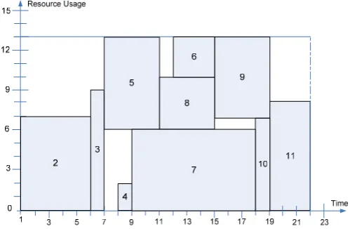
are problems which the software cannot find the optimum solution in MRT. As found in this table, LSP has the lowest value between all payments model and PEO has the greatest value for the objective function. Figures 1 to 4 show the Gantt chart of global\local optimum schedules for the first problem with various payment models.

5. SIMULATED ANNEALING

Simulated annealing (SA) [18] is a well-known local search meta-heuristic algorithm, which attempts to solve hard combinatorial optimization problems through a controlled randomization procedure. The ease of the use and provision of good solutions to real-world problems makes SA to be one of the most powerful and popular meta-heuristic algorithms to solve many optimization problems.

The SA algorithm starts with an initial solution for the given problem and repeats an iterative neighbor generation procedure that improves the objective function. During searching for the solution space and in order to escape from local minima, the SA algorithm offers the possibility to accept the worse neighbor solutions in a controlled manner. A neighboring solution (S') of the current solution (S) is generated in each iteration of the inner loop. If the objective function value of S' is better than S, then the generated solution replaces with the current one; otherwise, the solution can be also accepted with a probability

p

=

e

−ΔT_{. Where}

T

is the value of current temperature (i.e., higher values of

T

give a higher acceptance probability) and Δ= f(S)− f

( )

S′ . The acceptance probability is compared to a number y∈

(

0,1

]

generated randomly and S' is accepted whenever p > y.

5.1. Solution Representation

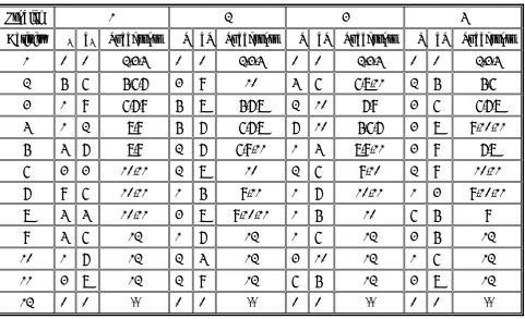
A feasible

TABLE 1. Input Data of Problems.

Problem 1 2 3 4

Activity dj uj Successors dj uj Successors dj uj Successors dj uj Successors

1 0 0 2,3,4 0 0 2,3,4 0 0 2,3,4 0 0 2,3,4

2 5 6 5,6,7 3 9 10 4 6 6,8,11 2 5 5,6

3 1 9 6,7,9 5 8 5,7,8 2 10 7,9 3 6 6,7,8

4 1 2 8,9 5 7 6,7,8 7 10 5,6,7 3 8 9,10,11

5 4 7 8,9 2 7 6,9,11 1 4 8,9,11 3 9 7,8

6 3 3 10,11 2 8 10 2 6 9,10 2 9 10,11

7 9 6 10,11 1 5 9,11 1 7 10,11 1 3 9,10,11

8 4 4 10,11 3 8 9,10,11 1 5 10 6 5 9

9 4 6 12 1 7 12 1 6 12 3 5 12

10 1 7 12 2 4 12 3 10 12 1 6 12

11 3 8 12 2 9 12 6 5 12 3 8 12

12 0 0 -- 0 0 -- 0 0 -- 0 0 --

TABLE 2. Positive and Negative Cash flows of Project Activities.

Activity 1 2 3 4 5 6 7 8 9 10 11 12 CFj+ 0 1225 908 821 1009 300 1031 910 964 1111 1177 0

CFj- 0 980 726 657 807 240 825 728 771 889 941 0

TABLE 3. Results of Solving the Given Problems with LINGO 8.

LSP PEO PEI PP Problem

Z CPU (S) Z CPU (S) Z CPU (S.) Z CPU (S.)

1 904.35 3549 1394.81 1183 1176.17* 3600 1272.03 540

2 1200.31 281 1544.69 331 1274.91* 3600 1332.30 1206 3 1078.14 233 1471.86 499 1175.55 3496 1401.67 1656 4 1191.17 3270 1456.50 1635 1286.23* 3600 1394.78* 3600

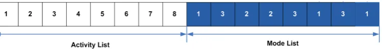
The (n + 1)-th element of the list defines the execution mode of the j-th elements (j = 1,…,n). Figure 5 presents a precedence feasible solution of a problem with eight activities. This list contains 16 elements where show the sequence of activities is 1 to 8 and activities 1, 6, and 8 execute in its first mode, activities 3 and 4 execute in second mode and other activities execute in its third mode.

5.2. Scheduling Generation Scheme

Scheduling generation schemes (SGS) are the core

of meta-heuristics for RCPSP\MMRCPSP and essential for generating feasible schedules. Therefore before presenting meta-heuristic algorithms for solving the model, we should define the SGS.

A comprehensive study on forward, backward and bi-directional planning strategies with various priority rule presented by Kelin 19. In forward planning, no activity is scheduled before all its predecessors have been finished. In backward planning an activity can schedule if and only if all Figure 1. Global optimum schedule of problem 1 with the

lump-sum payment (LSP) model.

Figure 2. Global optimum schedule of problem 1 with the

of its successors are scheduled. These strategies generate precedence feasible solutions. Bi-directional planning strategy constructs schedules in

forward and backward direction, simultaneously. There are two different SGSs that are available for each of these three strategies. The serial Figure 3. Local optimum schedule of problem 1 the with

payment on equal interval (PEI) model.

Figure 4. Global optimum schedule of problem with the

progress payment (PP) model.

scheduling scheme (SSS) constructs a feasible schedule in n stages, in each stage, one activity is selected and scheduled at the earliest precedence and resource feasible completion time. The parallel scheduling scheme (PSS) generates a feasible schedule in at most n iterations. More details about planning strategies and scheduling schemes are presented in Kelin 19 and Kolisch 20.

We extend the serial schedule generation scheme proposed by Kelin [19] for a multi-mode problem. A random selection is used for priority rule and also for the tie break rule because of unknown behavior of the objective function.

5.3. Starting Solution

A starting solution for

each instance is generated by setting all activities on the activity list in an ascending order that follows from the ordering of nodes in the precedence relation graph, and executing all activities in their first modes. This procedure has been commonly used in local search algorithms for the MRCPSP before.

5.4. Stopping Criterion

The stopping criterion

is defined as an known and constant number of visited solutions (i.e., an assumed number of computing the objective function values). It is worthy noting that the objective is to maximize the net present value (NPV).

5.5. Neighborhood Generation The neighbor

generation is performed by using one of the following two operators:

5.5.1. Activity shifting Assume that

) , , ; , ,

(A₁ A_n M₁ M_n

S = _{K K} be the current solution. An integer random number, a, is generated in the interval [1,n]. Let activity

A

_b be the last predecessor of activity

A

_a and

A

_c the first successor of in S. Another integer number, d, is generated randomly in the interval [b+1,c-1]. Now, a neighborhood solution is obtained by a cyclical shift of all the activities placed between a, d and also cyclical shift of these activities execution modes placed between n + a and n + d.

5.5.2. Mode changing an integer number, x, is

generated randomly in the interval [1,n]. The mode

of selected activity is changed to another one randomly chosen, if possible where the value of element n + x is changed.

In each transition, one of these operators is chosen randomly with an equal probability.

5.6. Cooling Scheme

The temperature can be controlled by a cooling scheme specifying how it reduces to make the procedure more selective as the search progresses to neighborhoods of good solutions. We decrease the temperature T in N steps, starting from an initial value T0 and using a

cooling factor

α

, 0<α <1. The initial temperature T0 needs to be high enough to allow the acceptance

of any new solution in the first step. In each iteration of N, the procedure generates a fixed number of solutions R and evaluates them by using the current temperature value, T =(1−α)T₀.

6. COMPUTATIONAL EXPRIMENT

In this section, we present the results of a computational experiment concerning the implementations of the meta-heuristic algorithm for the proposed model. The implementations are coded and compiled in MATLAB and run on Pentium 4 PC with CPU 4800 Hz and 512 MB RAM.

We use a set of benchmark instances generated using the project generator ProGen developed by Kolisch, et al [21]. The files with the mentioned instances are available in the project scheduling problem library PSPLIB.

with the smallest duration, and signing the lowest cash flow to mode with the biggest duration in each activity). Furthermore, the positive cash flow is generated with the uniform distribution in the interval [750,1500].

For all LSP, PEO, PEI, and PP models, the experiment is performed for two different values of the discount rate and holding cost rate. We assume that αi = {0.01,0.05} and αh = {0.005,0.01}. We

also assume that it is constant over the entire planning horizon.

For the PEI model, we additionally assume that different values of parameter H. The experiment is performed for H = {3,6}. For the PP model, we assume T = {4,8}. Thus, we have four combinations for the LSP and PEO models and eight

combinations for the PEI and PP models.

We determine the stopping criteria based on the problem size. This criteria is equal to 10n2 where n is a number of the non-dummy activity in each instance. Finally, we run our proposed SA algorithm 30 times for each combination of problem parameters. Taking into account that all the problem parameters are assumed in the experiment, as well as the number of instances from the PSPLIB library for a given number of activities, it is worthy to note that the algorithm is solved exactly as 60 × 30 × (4×2+8×2) = 43200 instances of the considered problems.

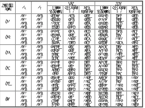
Table 4 illustrates the computational results of the LSP and PEO models, and Table 5 presents the results of the PEI and PP models.

TABLE 4. Computational Results for the LSP and PEO Models.

LSP PEO Problem

Size αi αh Best

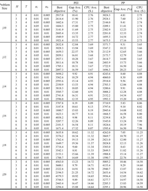
TABLE 5. Computational Results for the PEI and PP Models

PEI PP Problem

Size H T αi αh Best

objective Gap Ave. (%) CPU Ave. (S.) objective Best Gap Ave. (%) Ave. (S.) CPU

For each payment model considered in this paper, each value of αi and αh has an important impact on

the objective function of the project. If the other parameters of the problem remain fixed (i.e. the number of activities n for the LSP and PEO models, parameters (n ×H) and (n ×T) for the PEI and PP models, respectively), the net present value (NPV) decreases with the growth of αi and αh.

In the case of the PEI model with the fixed values of n, αi and αh, the amount of objective

function grows by increasing the value of parameter H. It is easy to see that an increase in the number of payments has to result in a better NPV of the project. It is just another way round for the PP model, the growth in the value of the interval length T results in worse NPV, which of course follows the fact that in this case the number of payments is decreased.

7. CONCLUSION

At the present time, organization tendency is to achieve greater benefit from project accomplishment. For this purpose they should reduce project cost and have better utilization of the resources. One way for cost reduction is completing each activity at the time that has minimum activity cost and maximum revenue for the organization. Based on this concept we present a new bi-objective model for multi-mode resource constrained project scheduling problem with discounted cash flows (MMRCPSPDCF) from contractor point of view with classical NPV and holding cost criteria. For better adoption of the real condition that organization deal with, we define both positive and negative cash flows and also consider different payment models for positive cash flows. This assumption related to more accommodation with real world that project managers are to deal with and help them to make better decisions.

8. ABBREVIATIONS

RCPSP Resource Constrained Project Scheduling Problem

MMRCPSP Multi-Mode RCPSP NPV Net Present Value

MILP Mixed-Integer Linear Program

LSP Lump-Sum Payment

PEO Payment at Event Occurrence PEI Payment at Equal time Interval

PP Progress Payment

MRT Maximum Running Time

SA Simulated Annealing

SGS Scheduling Generation Scheme SSS Serial Scheduling Scheme PSS Parallel Scheduling Scheme

9. ACKNOWLGEMENT

This study was partially supported by the University of Tehran under the research grant No. 8106043/1/06. The first author is grateful for this financial support.

10. REFERENCES

1. Kolisch, R. and Padman, R., “An Integrated Survey of Deterministic Project Scheduling”, Omega, Vol. 29,

(2001), 249-272.

2. Sprecher, A., Kolisch, R. and Drexl, “A., Semi-Active, Active, and Non-Delay Schedules for the Resource-Constrained Project Scheduling Problem”, European Journal of Operational Research, Vol. 80, (1995),

94-102.

3. Herroelen, W., Demeulemeester, E. and De Reyck, B., “A Classification Scheme for Project Scheduling, In: J. Weglarz (Ed.), Project Scheduling-Recent Models, Algorithms and Applications”, Boston: Kluwer Academic,

(1999), 1-26.

4. Russell, A. H., “Cash Flows in Networks”,

Management Science, Vol. 16, No. 5 (1970), 357-373.

5. Ulusoy, G., Serifoglo, F. S. and Sahin S., “Four Payment Models for the Multi-Mode Resource Constrained Project Scheduling Problem with Discounted Cash Flows”,

Annals of Operations Research, Vol. 102, (2001),

237-261.

6. Mika, M., Waligora, G. and Wezglarz, J., “Simulated Annealing and Tabu Search for Multi-Mode Resource-Constrained Project Scheduling with Positive Discounted Cash Flows and Different Payment Models”, European Journal of Operational Research, Vol. 164, (2005),

639-668.

8. Brinkmann, K. and Neumann, K., “Heuristic Procedures for Resource-Constrained Project Scheduling with Minimal and Maximal Time Lags: The Resource Leveling and the Minimum Project-Duration Problem”,

Journal of Decision Systems, Vol. 5, (1996) 129-55.

9. Bandelloni, M., Tucci, M. and Rinaldi, R., “Optimal Resource Leveling Using Non-Serial Dynamic Programming”, European Journal of Operational Research, Vol. 78, (1994), 162-177.

10. Najafi, A.A. and Niaki, S. T. A., “A genetic Algorithm for Resource InvestmentProblem with Discounted Cash Flows”, Applied Mathematics and Computation, Vol. 183, No. 2, (2006), 1057-1070.

11. Najafi, A. A. and Niaki, S. T. A., “Resource Investment Problem with Discounted Cash Flows”,

International Journal of Engineering, Vol. 18, No. 1, (2005), 53-64.

12. Shadrokh, S. and Kianfar, F., “A Genetic Algorithm for Resource Investment Project Scheduling Problem, Tardiness Permitted with Penalty”, European Journal of Operational Research, Vol. 181, No. 1, (2007),

86-101.

13. Icmeli, O. and Rom, W. O., “Ensuring Quality in Resource Constrained Project Scheduling”, European Journal of Operational Research, Vol. 103, (1997),

483-96.

14. Erengüc, S. S. and Icmeli, O., “Integrating Quality as a Measure of Performance in Resource-Constrained Project Scheduling Problems”, In J. Weglarz (Ed.), Project Scheduling Recent Models, Algorithms and

Applications, Boston: Kluwer Academic, U.S.A., (1999) 433-50.

15. Al-Fawzan, M. A. and Haouari, M., “A Bi-Objective Model for Robust Resource-Constrained Project Scheduling”, International Journal of Production Economics, Vol. 96, (2005), 175-187.

16. Kobylańki, P. and Kuchta, D., “A Note on the Paper by Al-Fawzan, M. A. and Haouari, M. About A Bi-Objective Problem for Robust Resource-Constrained Project Scheduling”, International Journal of Production Economics, Vol. 107, (2007), 496-501.

17. Zhenyuan, L. and Hongwei, W., “Heuristic algorithm for RCPSP with the Objective of Minimizing Activities’ Cost”, Journal of Systems Engineering and Electronics, Vol. 17, No. 1, (2006), 96-102.

18. Kirkpatrick, S., Gelatt, C. D. and Vecchi, M. P., Optimization by Simulated Annealing, Science, Vol.

220, (1983), 671-680.

19. Klein, R., “Bidirectional Planning: Improving Priority Rule-Based Heuristics for Scheduling Resource Constrained Projects”, European Journal of Operational Research, Vol. 127, (2000), 619-638.

20. Kolisch, R., “Serial and Parallel Resource-Constrained Project Scheduling Methods Revisited-Theory and Computation”, European Journal of Operational Research, Vol. 90, (1996), 320-333.