A ROBUST FEEDFORWARD ACTIVE NOISE CONTROL
SYSTEM WITH A VARIABLE STEP-SIZE FXLMS ALGORITHM:
DESIGNING A NEW ONLINE SECONDARY
PATH MODELLING METHOD
P. Davari
Department of Electrical and Computer Engineering, Babol Univesity of Technology P.O. Box 47144, Babol, Iran
H. Hassanpour*
School of Information Technology and Computer Engineering, Shahrood University of Technology P.O. Box 316, Shahrood, Iran
*Corresponding Author
(Received: October 29, 2007 – Accepted in Revised Form: May 9, 2008)
Abstract Several approaches have been introduced in literature for active noise control (ANC)
systems. Since Filtered-x-Least Mean Square (FxLMS) algorithm appears to be the best choice as a controller filter. Researchers tend to improve performance of ANC systems by enhancing and modifying this algorithm. This paper proposes a new version of FxLMS algorithm. In many ANC applications an online secondary path modelling method using a white noise as a training signal is required to ensure convergence of the system. This paper also proposes a new approach for online secondary path modelling in feedfoward ANC systems. The proposed algorithm is designed in a way that the injection of white noise is stopped at the optimum point, when the modelling accuracy is sufficient. In this approach, a sudden change in secondary path during the operation makes the algorithm to reactivate injection of the white noise to adjust the secondary path estimation. Benefiting new version of the FxLMS algorithm and not a continual injection of white noise during system operation makes the proposed system more desirable, also improves the noise attenuation and convergence rate. Comparative simulation results shown in this paper indicate effectiveness of the proposed approach.
Keywords Adaptive Filter, Active Noise Control, FxLMS, Online Modelling
ﻩﺪﻴﻜﭼ
ﺰﻳﻮﻧ ﻝﺎﻌﻓﻝﺮﺘﻨﮐﯼﺎﻫ ﻢﺘﺴﻴﺳﯼﺍﺮﺑﯼﺩﺎﻳﺯ ﯼﺎﻫﺵﻭﺭ ﻥﻮﻨﮐﺎﺗ (ANC)
ﺪﻧﺍ ﻩﺪﺷﯽﻓﺮﻌﻣ
.
ﻪﮐﯽﻧﺎﻣﺯ ﺯﺍ
ﻢﺘﻳﺭﻮﮕﻟﺍ FxLMS ﯽﻣﺵﻼﺗﻥﺎﻘﻘﺤﻣ،ﺖﺳﺍﻩﺪﺷﻪﺘﺧﺎﻨﺷﻩﺪﻨﻨﮐﻝﺮﺘﻨﮐﺮﺘﻠﻴﻓﯼﺍﺮﺑﺏﺎﺨﺘﻧﺍﻦﻳﺮﺘﻬﺑﻥﺍﻮﻨﻋﻪﺑ ﺎﺗﺪﻨﻨﮐ
ﻟﺍﻦﻳﺍﻥﺩﺮﮐﺮﺗﻪﻨﻴﻬﺑﺎﺑﺍﺭﺰﻳﻮﻧ ﻝﺎﻌﻓﻝﺮﺘﻨﮐﯼﺎﻫﻢﺘﺴﻴﺳﺩﺮﮑﻠﻤﻋ ﺪﻨﻫﺩﺀﺎﻘﺗﺭﺍﻢﺘﻳﺭﻮﮕ
.
ﺪﻳﺪﺟﻪﺨﺴﻧﮏﻳﻪﻟﺎﻘﻣﻦﻳﺍ
ﻢﺘﻳﺭﻮﮕﻟﺍﺯﺍ FxLMS
ﯽﻣﺡﺮﻄﻣ ﺍﺭ ﺪﻨﮐ
.
،ﺰﻳﻮﻧ ﻝﺎﻌﻓ ﻝﺮﺘﻨﮐﯼﺎﻫﺩﺮﺑﺭﺎﮐ ﺯﺍﯼﺭﺎﻴﺴﺑ ﺭﺩ ﯼﺍﺮﺑ
ﯽﻳﺍﺮﮕﻤﻫﺯﺍ ﻥﺎﻨﻴﻤﻃﺍ
ﻪﻳﻮﻧﺎﺛﺮﻴﺴﻣ ﯼﺯﺎﺳ ﻝﺪﻣﯽﻧﺁ ﺵﻭﺭ ﮏﻳ ﻢﺘﺴﻴﺳ ﻩﺪﻧﺮﻴﮔﺭﺎﮐ ﻪﺑ
ﺯﺎﻴﻧ ﺩﺭﻮﻣ ،ﯽﺷﺯﻮﻣﺁ ﻝﺎﻨﮕﻴﺳ ﻥﺍﻮﻨﻋ ﻪﺑ ﺪﻴﻔﺳ ﺰﻳﻮﻧ
ﺖﺳﺍ
.
ﺪﺟﺵﻭﺭ ﻪﻟﺎﻘﻣﻦﻳﺍ ﺰﻳﻮﻧ ﻝﺎﻌﻓﻝﺮﺘﻨﮐﺩﺭﻮﺧ ﺶﻴﭘﯼﺎﻫﻢﺘﺴﻴﺳ ﺭﺩﻪﻳﻮﻧﺎﺛﺮﻴﺴﻣﯼﺯﺎﺳﻝﺪﻣﯼﺍﺮﺑﯼﺪﻳ
ﺍ ﻪﺋﺍﺭ
ﯽﻣ ﻫﺩ ﺪ
.
ﯽﺒﺳﺎﻨﻣ ﻥﺍﺰﻴﻣﻪﺑ ﯼﺯﺎﺳ ﻝﺪﻣ ﺖﻗﺩ ﻪﮐ ﯽﻧﺎﻣﺯ ﺭﺩ ﺎﺗﺖﺳﺍ ﻩﺪﺷ ﯽﺣﺍﺮﻃﯼﺍ ﻪﻧﻮﮕﺑ ﯼﺩﺎﻬﻨﺸﻴﭘ ﻢﺘﻳﺭﻮﮕﻟﺍ ﺪﻴﺳﺭ ، ﺪﻨﮐ ﯼﺮﻴﮔﻮﻠﺟﻪﻨﻴﻬﺑ ﻪﻄﻘﻧ ﻡﺎﻧﻪﺑ ﯼﺍﻪﻄﻘﻧ ﺭﺩﺪﻴﻔﺳ ﺰﻳﻮﻧﻖﻳﺭﺰﺗ ﺯﺍ
.
ﺎﻧﺮﻴﻴﻐﺗﮏﻳ ،ﺵﻭﺭﻦﻳﺍ ﺭﺩ ﺭﺩﯽﻧﺎﻬﮔ
ﯽﻣﺐﺟﻮﻣﻢﺘﺴﻴﺳﺩﺮﮑﻠﻤﻋﻡﺎﮕﻨﻫﻪﻳﻮﻧﺎﺛﺮﻴﺴﻣ ﻢﺘﻳﺭﻮﮕﻟﺍﺎﺗﺩﻮﺷ
ﯼﺍﺮﺑ ﺪﻴﻔﺳﺰﻳﻮﻧﻖﻳﺭﺰﺗ،ﻪﻳﻮﻧﺎﺛﺮﻴﺴﻣﻦﻴﻤﺨﺗﺢﻴﺤﺼﺗ
ﺪﻨﮐﻝﺎﻌﻓًﺍﺩﺪﺠﻣﺍﺭ
.
ﻢﺘﻳﺭﻮﮕﻟﺍﺪﻳﺪﺟﻪﺨﺴﻧﺯﺍﯼﺮﻴﮔﻩﺮﻬﺑﺎﺑ FxLMS
ﻦﻴﺣﺭﺩﺪﻴﻔﺳﺰﻳﻮﻧﺪﺘﻤﻣﻖﻳﺭﺰﺗﺯﺍﺰﻴﻫﺮﭘﻭ
ﻣﻭﻩﺪﻳﺩﺮﮔﺮﺗﻩﺍﻮﺨﻟﺩﻩﺪﺷﻪﺋﺍﺭﺍﺵﻭﺭ،ﻢﺘﺴﻴﺳﺩﺮﮑﻠﻤﻋ ﺪﺑﺎﻳﺀﺎﻘﺗﺭﺍﯽﻳﺍﺮﮕﻤﻫﺥﺮﻧﻭﺰﻳﻮﻧﻒﻴﻐﻀﺗﻥﺍﺰﻴ
.
ﻪﻴﺒﺷﺞﻳﺎﺘﻧ
ﯽﻣﺪﻴﮐﺄﺗﯼﺩﺎﻬﻨﺸﻴﭘﺵﻭﺭﻥﺩﻮﺑﺮﺛﺆﻣﺮﺑﻪﻟﺎﻘﻣﻦﻳﺍﺭﺩﻩﺪﺷﻪﺋﺍﺭﺍﯼﺯﺎﺳ ﺪﻨﻨﮐ
.
1. INTRODUCTION
In recent years, active noise control (ANC) and
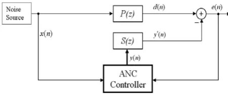
Figure 1. Block diagram of feedforward ANC system.
with equal amplitude and opposite phase replica primary noise (x(n) in Figure 1). Following the superposition principle, the result is cancellation or reduction of both noises [1]. ANC is a technique that efficiently attenuates low frequencies unwanted noises where passive methods are either ineffective or tend to be very expensive or bulky. ANC is based on either feedback structure, where the controller filter tries to reduce the unwanted noise without measuring the reference noise, or feedforward structure where the reference noise is captured (using reference sensor) before it passes through the acoustic path. Since the feedforward structure (Figure 1) measures primary noise (x(n) in Figure 1), it appears to be more efficient than the feedback structure in ANC applications. This is the reason that significant ANC improvements are mainly taken place for feedforward structure [1,3-5,8].
Non-linearity or inaccuracy in secondary path transfer function S(z), the path leading from the noise controller output to the error sensor measuring the residual noise, generally causes instability to the standard least mean square (LMS) algorithm. Several developments of the LMS algorithm have been introduced to solve this problem. In general, Filtered-x-Least Mean Square (FxLMS) algorithm is used to overcome the instability problem [1]. The FxLMS algorithm uses estimation of the secondary path to reimburse the problem raised by the transfer function. In practical cases the secondary path is usually time varying or non-linear, which leads to a poor performance or system instability. Therefore, online modelling of secondary path is required to ensure convergence of the ANC algorithm [5,7-9].
Most online secondary path modelling techniques entail injection of the additional random
noise as a training signal to afford the felicitous estimation of the secondary path [1]. White noise is usually utilized as an ideal training signal in modelling the secondary path [7-9].
The proposed system is based on a new version of FxLMS algorithm, as the main part of the system, and a new online secondary path estimator. In ANC applications, usually step size of the adaptive filter is set to a low value. This prevents the system to diverge when power of the reference signal x(n) is increased. However, once the power decreases the low value of the step size reduces the noise attenuation and convergence rate of the adaptive filter. Thus, if the step size could be increased when the power decreases, and vice versa, the system performance would be raised significantly. On the other hand, the step size could be correspondingly changed with power of the generated white noise, as it accordingly affects the convergence rate of the secondary path modelling [9]. This allows using a bigger step size during the system operation. By considering the above situations we propose a new technique in this paper which employs a varying step-size for the adaptive filter during the system operation.
Similar to other existing approach [3-8], the proposed algorithm uses white noise to model the secondary path. To increase performance of the algorithm in the secondary path modelling, we employ a new variable step size (VSS) LMS algorithm, as the first novelty for the proposed system. Secondly the VSS-LMS algorithm is stopped at the optimum point. We show that this technique could significantly improve performance of the system in noise attenuation. In addition, not continually having the white noise makes the system more desirable as continuous existence of the noise in the environment may have an unpleasant result.
estimation of the secondary path has no impact on the accuracy of the estimation.
The organization of this paper is as follows. In Section 2, the feedforward ANC system is briefly described. Section 3 introduces the online secondary path modeling method followed by the proposed approach. In Section 4, we illustrate our simulation results, and finally in Section 5 conclusions are drawn.
2. FEEDFORWARD ANC SYSTEM
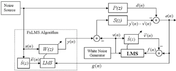
Block diagram of a feedforward FxLMS ANC system is shown in Figure 2 [1]. Here, P(z) is the primary path, the acoustic response from the reference noise source to the error sensor; and S(z) represents the secondary path. In this figure, Sˆ(z) is estimation of the secondary path S(z).
The secondary signal y(n) is generated as:
), n ( L x ) n ( T w ) n (
y = (1)
Where w(n)=[w0(n)w1(n)...wL−1(n)]T is the
tap-weight vector, and T 1)] L 1)...x(n [x(n)x(n (n) L
x = − − + is the L sample
reference signal vector. These coefficients are updated by the FxLMS algorithm as follows:
(n) xˆ (n)e(n) w μ (n) w 1) (n
w + = + ′ , μw >0, (2)
Where μw is the step size, and T )] 1 L n ( xˆ )... 1 n ( xˆ ) n ( xˆ [ ) n (
xˆ′ = ′ ′ − ′ − + is the filtered reference signal vector. The reference filtering signal through (z)Sˆ is:
(n) M (n)x T sˆ (n)
xˆ′ = (3)
Where sˆ(n)=[sˆ0(n)sˆ1(n)...sˆM−1(n)]T is the impulse response of the modelling filter Sˆ(z), and
T 1)] M 1)...x(n [x(n)x(n (n) M
x = − − + is an M
sample reference signal vector.
3. ONLINE SECONDARY PATH MODELING METHOD
3.1. Existing Approaches
3.1.1. Eriksson’s method The basic online secondary path modelling method which uses random noise as a training signal (Figure 3) was proposed by Eriksson, et al [3]. The authors have introduced a new adaptive filter to model S(z) during online operation of ANC system. The residual error signal e(n) of this algorithm is expressed as: ) n ( v ) n ( s ) n ( v ), n ( y ) n ( s ) n ( y (n), v (n) y d(n) e(n) ∗ = ′ ∗ = ′ ′ + ′ − = (4)
Where v(n) is an internally generated white Gaussian noise injected at the output of the control filter W(z).
In the Figure 3 Sˆ(z) is the modelling FIR filter with length M that generates vˆ′(n) expressed below: (n) M (n)v T sˆ (n)
vˆ′ = , (5)
Where sˆ(n)=[sˆ0(n)sˆ1(n)...sˆM−1(n)]T is the impulse response of the modelling filter Sˆ(z), and
T 1)] M 1)...v(n [v(n)v(n (n) M
v = − − + .
As the figure shows, vˆ′(n) generates the error signal for the modelling filter Sˆ(z) given as:
(n) vˆ (n)] v (n) y [d(n)
f(n)= − ′ + ′ − ′ (6)
The error signal used for the control filter W(z) is: (n)
v (n)] y [d(n)
g(n)= − ′ + ′ (7)
Coefficients of the modelling filter Sˆ(z) are updated as follows:
) n ( v ) (n )f n ( s μ ) n ( sˆ ) 1 n (
sˆ + = + (8)
Figure 2. Block diagram of a feedforward FxLMS ANC system.
Figure 3. Eriksson’s method for online secondary path modeling [3].
control filter W(z) are updated as below: (n)
xˆ (n)e(n) w
μ
w(n) 1)
w(n+ = + ′ (9)
3.1.2. Zhang’s method Several methods have later been proposed which improved performance of the Eriksson’s method [3-8]. All of these approaches enhanced the online secondary path modelling method to increase the modelling accuracy. To achieve this result an additional white noise, v(n), is needed. Such an additional noise has no correlation with the primary noise and hence cannot be attenuated or cancelled by the ANC system. Thus, the introduced enhancements in these methods are in such a way to control the injected noise (v(n)).
Here we briefly described Zhang, et al [6] who obtained good performance. Consider Figure 4 which shows Zhang’s method for an ANC system. This method is based on a set of cross-updated adaptive filters, W(z), Sˆ(z), C(z). The error signal,
g(n), for the control filter W(z) is expressed as: (n)
vˆ (n) v (n) y d(n)
g(n)= − ′ + ′ − ′ (10)
This error signal is also used to update third filter C(z). This filter generate an output signal u(n) used in error signal of LMS algorithm associated with
) z (
Sˆ which is given as:
) n ( u ) n ( vˆ ) n ( v ) n ( y ) n ( d ) n (
f = − ′ + ′ − ′ − (11)
When C(z) converge, u(n)≈g(n)⇒f(n)→0 which is exactly the desired event.
This method obtained high performance as described in [6]; however, it increased the design complexity of the ANC system. The complexity cost of the system decreases the noise reduction performance and convergence rate of secondary path modelling.
Figure 4. Zhang’s method [6] for online secondary path modeling.
Figure 5. Akhtar’s method [8] for online secondary path modeling.
online secondary path modelling methods, the method presented by Akhtar, et al [8] appears the best choice. This method achieved a high performance with lower complexity.
Akhtar’s method (Figure 5) is a modified version of Eriksson’s method [3]. This method utilizes VSS-LMS algorithm for modelling filter and uses f(n) as error signal for both Sˆ(z) and W(z).
The VSS-LMS algorithm is used to update modelling filter Sˆ(z) coefficients. For more detail on theory of this algorithm readers may refer to [8]. The modelling filter in (8) is updated using the step-size parameter (μs(n)) of VSS-LMS algorithm and this parameter is calculated using the following three steps [8]:
• Initially, the power of error signals e(n) and f(n) are computed:
(n) 2
λ)e (1 1) (n e
λP (n) e
P = − + −
(n) 2
λ)f (1 1) (n f
λP (n) f
P = − + − , 0.9<λ<1. (12) • Then, the ratio of the estimated powers is obtained:
(n) e (n)/P f P
ρ(n)=
1
ρ(0)≈ , limn→∞ρ(n)→0 (13)
• Finally, the step size is calculated as follows:
max s
ρ(n))μ
(1 min s
ρ(n)μ
(n) s
μ = + − , (14)
where
max s
μ
, min s
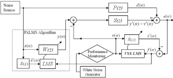
Figure 6. Proposed method for ANC feedforward systems with online secondary path modeling.
3.2. Proposed Method
Here we suggest a new version of the FxLMS algorithm to increase noise attenuation and convergence rates. To improve the performance, the adaptive filter step size μwadaptively changes the following power variations of the reference noise and the generated white noise alike. In addition, a new online secondary path modelling on the basis of VSS-LMS algorithm is proposed in this paper.
Figure 6 shows the proposed system block diagram. Usually μw in (9) is set to a low value. This prevents the system to diverge when power of the reference signal x(n) is increased.
However, once the power decreases the low value of μw reduces the noise attenuation and
convergence rate of the adaptive filter (W(z)). Thus, if μw could be increased when the power
decreases, and vice versa, the system performance would be risen significantly. On the other hand, the step size μw can correspondingly be changed with the power of the generated white noise, as online estimation of the secondary path is used. When power of the generated white noise increases, the secondary path modelling convergence rate raises [9]. This allows using a bigger μw during the system operation. By considering the above situations we propose the following procedure to vary the step-size (μw) during the system operation.
Let consider ) n ( x P
) n ( v P
, where Pv(n) and Px(n) represent power of the generated white noise v(n)
and the reference signal x(n), respectively. By adding this new term to (9) the filter step size adapts with the power variations of the above signals:
(n) xˆ (n)f(n) w
μ
(n) x P
(n) v P w(n) 1)
w(n+ = + ′ (15)
We estimate power of these signals as:
(n) 2
γ)x (1 1) (n x
γP (n) x
P = − + − ,
(n) 2
γ)v (1 1) (n v
γP (n) v
P = − + − , (16)
Where γ is the forgetting factor (0.9 < γ <1). The online secondary path estimations are the same as Akhtar’s method, except we add the above new term to (13) to maintain μs variations with
w
μ as follows:
(n) e P (n) x P
(n) f P (n) v P
ρ(n)
+ +
= (17)
Here, the VSS-LMS algorithm is briefly described to show the way, which the optimum point is obtained. The VSS-LMS algorithm is initially set to a small step size. During the process of this algorithm, μs is increased as the error signal f(n) decreases and vice versa. It needs to be noted that any increase of the step size corresponds to a faster convergence of the adaptive algorithm. Consequently, once W(z) is slow in reducing e(n), the step size remains small which results in a lower convergence rate. Hence, the modeling filter,Sˆ(z), converges to a good estimation when f(n) decreases. This happens when μs increases as high as
max s
μ .
Thus, the injection of the white noise is stopped at the optimum point which is measured using:
α
s
μ
max s
μ − < , 1×10⁻⁵<α≤1×10⁻⁴ (18)
As can be seen from Figure 6, this condition validity is monitored at the performance monitoring stage. By settingα to a lower value,
the modelling error as well as the convergence rate is decreased, which results in an accurate modelling of the secondary path.
In some practical cases the secondary path may suddenly change. This event derives the system to diverge. To prevent such effects, Sˆ(z) needs to be updated. Existing online secondary path modelling techniques [3-8] control the secondary path changes during system operation by continuous injection of the white noise. As described before, in the proposed method injection of the white noise is stopped at the optimum point. To adapt the system with the secondary path changes, the proposed algorithm is designed in such a way that it can monitor the secondary path variations by the following expression:
0 f(n) 10 log
20 < (19)
If the validity of the above equation is not satisfied, the system reactivates the VSS-LMS algorithm and injects the white noise to remodel Sˆ(z). The same as before, the injection is stopped at the optimum point using (18). The above procedure is repeated during the system operation to adapt the algorithm
with characteristics of the environment. Figure 7 simply shows procedure of the proposed algorithm. It is important to note that all of the primary values of the estimated powers in (12) and (16) are set to 1 at the initialization step.
Estimation of the secondary path can be obtained by using the off-line modeling method followed by an online modeling. Off-line estimation improves convergence rate and consequently noise reduction. Existing methods [7,8] usually use off-line estimation prior to online modeling. However, as mentioned before, in some applications the primary noise exists even during the off-line modeling in which adversely affects the accuracy of the modeling filter. Therefore, the proposed approach has this ability that, without using the offline estimation, maintains convergence rate and the noise reduction performance of the system.
4. SIMULATIONS RESULTS AND PERFORMANCE EVALUATION
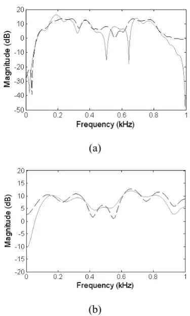
In this section the proposed ANC system is simulated using Matlab version 7.1. In this simulation, we have used the primary path P(z) and secondary path S(z) of the experimental data provided in [2]. The magnitude responses of the primary and secondary paths are shown in Figure 8. Using these data, P(z) and S(z) are considered as FIR filters with tap–weight lengths 48 and 16 respectively. Rate of the sampling frequency in this simulation was 2 kHz. Comprehensive experiments have been performed to find appropriate values for a fast and stable performance of the ANC system. Length of FIR filter Sˆ(z) for modelling the secondary path, and length of the adaptive filter W(z) used for the noise cancellation have been chosen 16 and 32, respectively.
In this simulation performance of the proposed method is compared with that of Eriksson’s [3], Akhtar’s [8] and Zhang’s method [6]. Simulations parameters for all of the four methods are set as described in Table 1.
Figure 7. The proposed feedforward ANC algorithm.
(a)
(b)
Figure 8. Magnitude response of the acoustic paths (Solid
line: original path, dashed line: the changed path at n = 20,000): (a) Magnitude response of the primary path P(z), (b) Magnitude response of the secondary path S(z).
In case 1, performance of the proposed method is compared by using two different noises. Case2 shows advantage of the proposed method in not using off-line estimation of secondary path. Finally case 3 indicates effectiveness of the proposed algorithm in maintaining its performance against sudden changes of the acoustic paths behaviour. To signify performance of the system on noise reduction the following equation is used:
⎟ ⎟ ⎠ ⎞ ⎜
⎜ ⎝ ⎛
∑ ∑ −
=
(n) 2 d (n) 2 e 10 10log
R (20)
The larger the positive value of R indicates the more noise reduction is achieved. To show the convergence rate and modelling accuracy of the system the relative modelling error is used as defined below:
⎪ ⎪ ⎭ ⎪ ⎪ ⎬ ⎫
⎪ ⎪ ⎩ ⎪ ⎪ ⎨ ⎧
∑− = ∑−
= −
=
1 M
0 i
2 (n)] i [s 1 M
0 i
2 (n)] i sˆ (n) i [s
10 10log
ΔS(dB) (21)
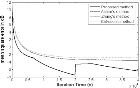
All the results shown in each case have been obtained as an average five different experiments. It is interesting to note that in all of these cases both Akhtar’s method and Zhang’s method obtain the same noise reduction (20) and Mean Square Error (MSE), while their modelling error (21) are different (see Figures 9-16).
4.1. Case 1
In this case, Akhtar’s method is evaluated under the situations defined by the authors in [8], and parameters for Eriksson’s and Zhang’s methods are set for the most proper situation. To set the initial value for Sˆ(z) (sˆ(0)), off-line secondary path modeling is performed. The off-line modeling is stopped when the modeling error (20) is reduced to-5 dB.TABLE 1. Simulation Parameters for the Four Approaches.
Eriksson’s method ) s , w
(μ μ 5×10−4,1×10−2
Akhtar’s method ) , min s , max s , w
(μ μ μ λ
99 . 0 , 4 10 75
, 3 10 25 , 4 10 5
− ×
− × − ×
Zhang’s method ) h , s , w
(μ μ μ 2
10 1
, 2 10 1 , 4 10 5
− ×
− × − ×
Proposed method ) min s
μ
, max s
μ
, w (μ
(λ,γ,α)
3 10 9 , 2 10 4 , 3 10
2× − × − × −
4 10 7 , 999 . 0 , 99 .
0 × −
(a)
(b)
Figure 9. Simulation results using first experiment in Case1.
(a) Noise reduction versus iteration time (n), (b) Relative modeling error versus iteration time (n).
Figure 10. Comparing the error curves of the proposed method with that of the other three existing approaches using first experiment in Case1.
positively. As can be seen from the figure, compared with the other three methods the proposed method offers a better noise reduction and convergence rates.
In the next experiment the reference noise is a narrowband signal comprising frequencies of 100, 200, 300 and 400 Hz. Same as the previous experiment, its variance is adjusted to 2, and a white noise with SNR of 30 dB is added.
The results comparison of this experiment are shown in Figures 11 and 12. These results also show superiority of the proposed method over the existing approaches in attenuating narrowband noises.
4.2. Case 2
As mentioned before, using off-line estimation prior to online modeling procedure may cause problems for ANC system. However, not using off-line estimation decreases convergence rate and may affect modeling accuracy.(a)
(b)
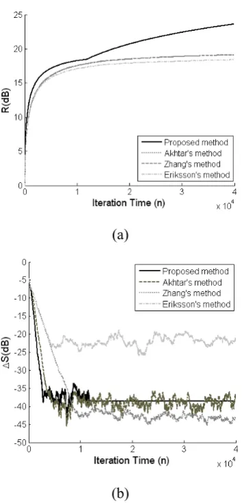
Figure 11. Comparing simulation results of the proposed
method with that of the other three existing approaches using second experiment in Case 1. (a) Noise reduction versus iteration time (n), (b) Relative modeling error versus iteration time (n).
Figure 12. Comparing the error curves of the proposed
method with that of the other three existing approaches using second experiment in Case 1.
(a)
(b)
Figure 13. Comparison simulation results for the proposed
algorithm in Case 2 with that of the other three existing approaches using the second experiment in Case 1. (a) Noise reduction versus iteration time (n), (b) Relative modeling error versus iteration time (n).
(a)
(b)
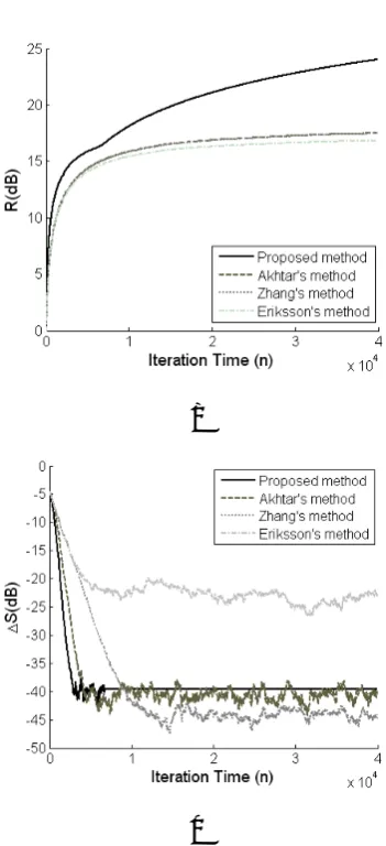
Figure 15. Comparison simulation results for the proposed
algorithm in Case 3 with that of the other three existing approaches using the first experiment in Case 1. (a) Noise reduction versus iteration time (n), (b) Relative modeling error versus iteration time (n).
Figure 16. Comparing the error curves of the proposed
method with that of the other three existing approaches using first experiment in Case 1.
seen, without using off-line estimation, the proposed method could achieve a better performance compared to the other methods.
In this experiment Figure 13a and 14 indicate the effect of not continually injecting, the white noise on the basis of noise reduction and MSE, respectively.
4.3. Case 3
In this case, it is assumed that boththe primary and the secondary paths transfer functions are suddenly changed during the operation. Figure 8 shows the magnitude response of the original and changed path. In this figure, the solid line represents the secondary path at start point, n = 0, and the dashed line represents the changed path at iteration n = 20000. Here we consider the reference signal used in the first experiment of case 1. In this experiment, we use the off-line estimation of the secondary path utilized in case 1.
The result of noise reduction (20) and modeling error (21) for the three approaches are shown in Figure 15a,b respectively. As can be seen the proposed method maintains its performance with a higher convergence rate. The importance is that the proposed method achieves a higher noise reduction (R) compared to the other methods. For more studies on the ANC system behavior we illustrated the simulation result on the basis of MSE in Figure 16.
5. CONCLUSIONS
This paper proposed a new ANC system with online secondary path modelling. The proposed system is based on a new version of FxLMS algorithm as main part, and a modified variable step size (VSS) LMS algorithm is used to adapt the modelling filter of the secondary path. Preventing continuous injection of the white noise increases the performance of the proposed method significantly and makes it more desirable for practical ANC systems. Computer simulations have been conducted for a single-channel feedforward ANC system. Comparative result shown in this paper demonstrated effectiveness of the proposed method.
complicated situation and increased the modelling accuracy as well as noise reduction.
6. REFERENCES
1. Kuo, S. M. and Morgan, D. R., “Active Noise Control: a Tutorial Review”, Proc. of IEEE, Vol. 8, No. 6, (1999),
943-973.
2. Kuo, S. M. and Morgan, D. R., “Active Noise Control
Systems-Algorithms and DSP Implementation”, New York, U.S.A., (1996).
3. Eriksson, L. J. and Allie, M. C., “Use of Random Noise for On-Line Transducer Modeling in an Adaptive Active Attenuation System”, J. Acoust. Soc. Amer, Vol.
85, No. 2, (1989), 797-802.
4. Bao, C., Sas, P. and Brussel, H. V., “Adaptive Active Control of Noise in 3-D Reverberant Enclosure”, J.
Sound Vibr., Vol. 161, No. 3, (1993), 501-514.
5. Gan, W. S. and Kuo, S. M., “An Integrated Audio and
Active Noise Control Headsets”, IEEE Trans.
Consumer Electron, Vol. 48, No. 2, (2002), 242-247.
6. Zhang, M., Lan, H. and Ser, W., “Cross-Updated Active Noise Control System with Online Secondary Path Modeling”, IEEE Trans. Speech, Audio Proc., Vol. 9,
No. 5, (2001), 598-602.
7. Akhtar, M. T., Abe, M. and Kawamata, M., “A New
Variable Step Size LMS Algorithm-Based Method for Improved Online Secondary Path Modeling in Active Noise Control Systems”, IEEE Trans. Audio., Speech
Lang. Processing, Vol. 14, No. 2, (2006), 720-726.
8. Akhtar, M. T., Abe, M. and Kawamata, M., “A Method
for Online Secondary Path Modeling in Active Noise
Control Systems”, Proc. IEEE International
Symposium on Circuits and Systems (ISCAS ’05), Vol.
1, (2005), 264-267.
9. Kuo, S. M. and Vijayan, D., “Optimized Secondary Path Modeling Technique for Active Noise Control Systems”, IEEE Asia-Pacific Conference on Circuits
![Figure 4. Zhang’s method [6] for online secondary path modeling.](https://thumb-us.123doks.com/thumbv2/123dok_us/241182.2018834/5.595.129.465.574.701/figure-zhang-s-method-online-secondary-path-modeling.webp)