Image Quality Enhancement Using Pixel Wise Gamma Correction

IMAGE QUALITY ENHANCEMENT USING PIXEL-WISE

GAMMA CORRECTION

H. Hassanpour* and S. Asadi Amiri

Department of Computer Engineering, University of Shahrood Technology, Shahrood, Iran [email protected], [email protected]

*Corresponding Author

(Received: September 14, 2011 – Accepted in Revised Form: October 20, 2011)

doi: 10.5829/idosi.ije.2011.24.04b.01

value of its individual pixels. Most of existing gamma correction methods apply a uniform gamma value across the image. Considering the fact that gamma variation for a single image is actually nonlinear, the proposed method locally estimates the gamma values in an image

database of training images are constructed from various standard images under different gamma conditions. Then by windowing each of the training images, a number of features that characterize images content are computed from its pixel intensity histogram, gray level co-occurrence matrix, and discrete cosine transform domain. To improve the gamma values of an image the aforementioned features are initially computed in sliding windows, then SVM is employed to estimate the gamma value in each window. In this study, it is shown that the proposed method has performed well in improving the quality of images. Subjective and objective image quality assessments used in this study attest superiority of the proposed method compared to the existing methods in image quality enhancement using image gamma value.

Keywords Image Enhancement, Gamma Correction, Feature Selection, SVM.

1. INTRODUCTION

Image quality enhancement algorithms are developed to improve the visual appearance of an image by increasing the contrast, adjusting brightness, and enhancing visually important features [1]. Image enhancement is very important pre-processing stage in most image processing applications. For example in face recognition systems, the algorithms may fail to recognize faces correctly due to changes in illumination [2, 3]. Many devices used for capturing, printing or displaying the images generally apply a

transformation, called power-low [4], on each pixel of the image that has a nonlinear effect on luminance:

 



u u

g  (1)

In the above equation u _ϵ [0, 1] denotes the image pixel intensity; γ is a positive constant introducing the gamma value. By this assumption, the value of γ typically can be determined experimentally, by passing a calibration target with a full range of known luminance values through the imaging device. When the value of γ is known, .ﺖﺳﺍﻩﺪﺷﻡﺎﺠﻧﺍﺎﻣﺎﮔﺎﺑﺮﻳﻮﺼﺗﻱﺯﺎﺴﻬﺑﺩﻮﺟﻮﻣﻱﺎﻫﺵﻭﺭﻪﺑﺖﺒﺴﻧﻱﺩﺎﻬﻨﺸﻴﭘﺵﻭﺭﻱﺮﺗﺮﺑﻥﺩﺍﺩ

ﻥﺎﺸﻧ ﻱﺍﺮﺑ ﻲﻔﻴﮐﻭﻲﻤﮐ ﻲﺑﺎﻳﺯﺭﺍ ﻱﺎﻫﺭﺎﻴﻌﻣ .ﺩﺭﺍﺩ ﺮﻳﻭﺎﺼﺗ ﻱﺯﺎﺴﻬﺑﺭﺩﻲﺑﻮﺧ ﻲﻳﺍﺭﺎﮐﻱﺩﺎﻬﻨﺸﻴﭘ ﺵﻭﺭ ﻪﮐﺖﺳﺍ ﻩﺪﺷﻩﺩﺍﺩ ﻥﺎﺸﻧ ﻖﻴﻘﺤﺗﻦﻳﺍ ﺭﺩ .ﺩﻮﺷﻲﻣ ﻩﺩﺯﺐﻳﺮﻘﺗﻥﺎﺒﻴﺘﺸﭘ ﺭﺍﺩﺮﺑﻦﻴﺷﺎﻣ ﻂﺳﻮﺗﻩﺮﺠﻨﭘ ﺮﻫﻱﺎﻣﺎﮔ ﺭﺍﺪﻘﻣ ﺲﭙﺳ ،ﺩﻮﺷﻲﻣ ﺝﺍﺮﺨﺘﺳﺍ ﺮﻳﻮﺼﺗ ﻩﺮﺠﻨﭘ ﺮﻫ ﺯﺍ ﺎﻫﻲﮔﮋﻳﻭﻦﻴﻤﻫ ﺍﺪﺘﺑﺍ ،ﺪﻳﺪﺟ ﺮﻳﻮﺼﺗ ﻱﺯﺎﺴﻬﺑﻱﺍﺮﺑ .ﻢﻴﻳﺎﻤﻧﻲﻣ ﺝﺍﺮﺨﺘﺳﺍ ﺮﻳﻮﺼﺗﻲﺳﻮﻨﻴﺴﮐ ﻪﻔﻟﻮﻣ ﻭﺩﺍﺪﺧﺭﻢﻫﺲﻳﺮﺗﺎﻣ ،ﻡﺍﺮﮔﻮﺘﺴﻴﻫ ﺯﺍ ﻲﮔﮋﻳﻭ ﻱﺩﺍﺪﻌﺗ ﻭﻩﺩﺮﮐ ﻱﺭﺍﺬﮔﻩﺮﺠﻨﭘﺍﺭ ﻲﺷﺯﻮﻣﺁ ﺮﻳﻭﺎﺼﺗ ﻦﻳﺍ ﺯﺍ ﮏﻳ ﺮﻫ ﺲﭙﺳ .ﻢﻴﻳﺎﻤﻧﻲﻣ ﺩﺎﺠﻳﺍ ﺩﺭﺍﺪﻧﺎﺘﺳﺍ ﻒﻠﺘﺨﻣﺮﻳﻭﺎﺼﺗ ﺯﺍ ﺎﻣﺎﮔﺕﻭﺎﻔﺘﻣ ﺮﻳﺩﺎﻘﻣ ﺎﺑ ﻲﺷﺯﻮﻣﺁ ﺮﻳﻭﺎﺼﺗ ﺯﺍﻱﺍﻩﺩﺍﺩ ﻩﺎﮕﻳﺎﭘ ﺍﺪﺘﺑﺍ .ﺩﺮﻴﮔﻲﻣ ﻡﺎﺠﻧﺍﻥﺎﺒﻴﺘﺸﭘ ﺭﺍﺩﺮﺑﻦﻴﺷﺎﻣ ﮏﻤﮐﻪﺑ ﻲﻠﺤﻣ ﺕﺭﻮﺻﻪﺑﺎﻣﺎﮔ ﺡﻼﺻﺍﻪﻟﺎﻘﻣ ﻦﻳﺍﺭﺩ،ﺪﺷﺎﺑﻪﺘﻓﺮﮔﻡﺎﺠﻧﺍﻲﻄﺧﺮﻴﻏﺕﺭﻮﺻﻪﺑﺖﺳﺍﻦﮑﻤﻣ ﺮﻳﻮﺼﺗﺭﺩﺎﻣﺎﮔﺕﺍﺮﻴﻴﻐﺗﻪﮐﻲﻳﺎﺠﻧﺁﺯﺍ .ﺪﺑﺎﻳﻲﻣﺮﻴﻴﻐﺗ ﺮﻳﻮﺼﺗﮏﻳﻱﺎﻫﺖﻤﺴﻗﻡﺎﻤﺗﺭﺩﺖﺧﺍﻮﻨﮑﻳﺭﻮﻃﻪﺑﺎﻣﺎﮔﺐﻳﺮﺿ،ﺎﻣﺎﮔﺡﻼﺻﺍﺩﻮﺟﻮﻣﻱﺎﻫﺵﻭﺭﺮﺜﮐﺍﺭﺩ .ﺖﺳﺍﻩﺪﺷ ﻪﺋﺍﺭﺍﻞﺴﮑﻴﭘﺮﻫﻱﺍﺮﺑﺎﻣﺎﮔﺭﺍﺪﻘﻣﻦﻴﻴﻌﺗﺎﺑﺮﻳﻮﺼﺗﻱﺯﺎﺴﻬﺑﻱﺍﺮﺑﻱﺪﻳﺪﺟﮏﻴﺗﺎﻣﻮﺗﺍﺵﻭﺭﻪﻟﺎﻘﻣﻦﻳﺍﺭﺩ

ﻩﺪﻴﻜﭼ

VIA SVM CLASSIFIER

inverting this process is trivial:

 

1

1

u u

g  (2)

Often such calibration is not available or direct access to the imaging device is not possible, for example when an image is downloaded from the web. Also, most commercial digital cameras dynamically vary the amount of gamma [5]. Hence an algorithm is needed to reduce the effects of these nonlinearities, without any knowledge about the imaging device.

In addition to this problem, in practice, these nonlinear effects aren’t consistent across all regions of the image. In other words, the value of gamma may change from one region to another [9]. For instance, it is possible that a scene contains a large dynamic illumination range that an imaging device is not able to adequately capture. Thus, especially in very dark or bright regions of the image, some details may become clustered together within a small intensity range [6]. Hence a local enhancement process adjusts the image quality in di_fferent regions in a way that the human viewers grasp these details.

Image enhancement can be divided into two categories: spatial domain methods and frequency domain methods. The spatial domain methods operate on image pixels directly, such as: histogram equalization [7, 8], gamma correction [3, 5, 9, 10], partial differential equation (PDE) based method [11-12], retinex filter [13-15]. The frequency domain methods directly operate on the frequency domain such as: unsharp masking [16], combining nonlinear lowpass and highpass filters [17], homomorphic filter [18-19].

As mentioned above, imaging devices apply the power low transformation on each pixel of the image; hence gamma correction is required to enhance the image.

Recently, some algorithms [3, 5, 8, 9] have been developed to determine image gamma values. In [5] a blind inverse gamma correction technique was developed exploiting the fact that gamma correction introduces specific higher-order correlations in the frequency domain. In this approach the gamma values from 0.1 to 3 are applied to image pixels in 128×128 windows so that the best gamma value is the one that minimizes those higher order correlations. It means

that the image with a proper luminance has a minimum correlation. But unfortunately this method is time consuming and has limited success. In [3] a mapping function is considered to correlate gamma values with pixel values. In fact, the algorithm is a nonlinear transformation that makes pixels with low values brighter, whereas pixels with high values become darker. This transformation leaves midtons with less correction or even no correction. This approach is a pixel wise operation that may be successful on reducing the illumination on the scene. Since local information of the pixels is not used, image distortion may occur in natural images.

In this paper, we present a technique for estimating the gamma values without any calibration information or knowledge of the imaging device in a local approach. In this method, the training images are constructed from nine standard images under different gamma conditions, varying from 0.2 to 2.4. A sliding window of size 64×64 is moved across each image, then a number of features that related to image contents are computed from each window to train the support vector machine (SVM).

To modify the gamma values of an image, the same features are computed in a sliding window moving across the image. Then, SVM is employed to estimate the appropriate gamma values of each window. Finally, by applying the inverse of these

gamma values to image pixel intensity, the image with a proper luminance will be achieved.

In the next section, feature selection for the proposed gamma correction is described. In Section 3, SVM classifier is briefly described. Image quality assessment is introduced in Section 4. The proposed algorithm is presented in Section 5. Section 6 shows the results, and Section 7 contains the conclusions.

2. GAMMA CORRECTION AND FEATURE SELECTION

original image; and when the amount of γ is greater than one, the transformed image becomes darker than the original image. According to [20], the image contents can be described with a number of features in terms of luminance distribution, spatial orientation and frequency energy distribution. They can be grouped into three classes:

1. Feature derived from the histogram.

2. Features derived from the gray level co-occurrence matrix (GLCM).

3. Features derived from discrete cosine transform (DCT) domain.

In the following subsections, each category and the extracted features are discussed.

2.1. Pixel Intensity Histogram Histogram

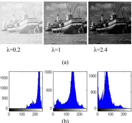
demonstrates the probabilistic distribution of gray levels within an image [20]. Figure 1 shows three different gamma condition images with their histograms. It reveals that, when the amount of γ is less than one, pixel intensity histogram has a peak at the right side of the histogram (lighter values), and when the amount of γ is greater than one the pixel intensity histogram has a peak at the left side of histogram (darker values).

λ=0.2 λ=1 λ=2.4

(a)

(b)

Figure 1. An image with three different gamma conditions and their associated histograms.

Also when the value of γ is around one, pixel intensity histogram has a peak at the center. This figure indicates that histogram has useful

information for image gamma correction. According to Equation (3), mean pixel intensity is calculated from the normalized histogram, H(g). This feature represents the histogram.





g

g gH

Mean ( ) (3)

where

1 ,..., 0 , 2 * 1 / )

(g Ng L L g nl 

H (4)

where g denotes a generic gray level value of a pixel, nlindicates the number of such levels (for

8-bit images nl=256), and Ng is the number of pixel

with a gray level g. L1×L2 represents the number of pixels in the image.

2.2. The Gray Level Co-Occurrenc Matrix

The gray level co-occurrence matrix is regarded as a two dimensional matrix. Its size is equal to the number of gray levels in an image. For instance, 256 discrete gray levels exist in the images used in this paper; thus, the GLCM for these images is a matrix of size 256×256 [21]. In contrast to histogram, GLCM describes the relationship between the values of neighbouring pixels. It measures the probability that a pixel of a particular gray level occurs at a specified direction and a distance from its neighbouring pixels. This can be calculated by the function P (i, j, d, Ө), where i is the gray level at location of coordinate (x, y), j is the gray level of its neighbouring pixel at a distance d and a direction Ө from a location (x, y) [22]. Ө usually ranges from: 0, 45, 90, to 135 [21]. This is mathematically defined by the Equation(5):





 









,

 

,



,





,

 

, ,





}

, , , , ,

, { # ) , , , (

2 2 1 1 2

2 1 1

2 2 1

1 2 2 1 1

 

 

 

 



y x y x d y x y x

j y x f i y x f y x y x d

j i

P (5)

In [23], fourteen different features of GLCM have been defined. These features consist of texture information, but, there may be correlation between them. Thus, the entire set of 14 features is not needed to be considered [24]. Considering a gray level co-occurrence matrix P, the definitions of the features used in this paper are as follows:

 Correlation

  

256 256( )( ) (, )

i j

j i

j i j pi j

i COR     ₍₆₎  Contrast:

Contrast feature is the amount of local variations present in an image.





256 256_{( )}2 _{(, )}

i j j i p j i CON (7)

 Homogeneity:

Homogeneity is a value that measures the closeness of the distribution of elements in the gray level co-occurrence matrix.



_{ }

256 256

1 ) , (

i j i j j i p HOM (8)  Energy:



256 256 _{(, )}2

i j

j i p

ENR (9)

Energy is the sum of squared elements.

2.3. Discrete Cosine Transform Information on

image complexity can be derived from the image’s frequency energy content, which is described by the discrete cosine transform [25].It is a technique for changing a signal into elementary frequency components [26]. It represents an image as a sum of sinusoids of different magnitudes and frequencies. With an input image, f, the DCT coefficients for the transformed output image, D, are computed according to Equation (10). In the equation, f, is the input image of N×M pixels, f(n, m) is the intensity of the pixel in row n and column m of the image, and y(u, v) is the DCT coefficient in row u and column v of the DCT matrix [26].

          



    M N v y M N u x y x f v u v u D N x M y * ) 1 2 ( cos * ) 1 2 ( cos ) , ( ) ( ) ( ) , ( 1 0 1 0     ₍₁₀₎ Where            1 ,..., 2 , 1 1 0 2 1 ) ( N u u u             1 ,..., 2 , 1 1 0 2 1 M v v v  (11) (12) The element in the upper left corner D(0,0) is called the DC coefficient, and the other elements are called AC coefficients. The average of original image is represented by the DC coefficient and variations in gray values in certain directions at certain rates are represented by the AC coefficients. The basis functions corresponding to the coefficients D (u,v) are respectively arranged in order of increasing spatial frequencies from the upper left to the lower right corner in the horizontal and vertical spatial dimensions [6]. We compute four following features from DCT matrix D. These features represent image brightness over total variation (F_DC), vertical variation over total variation (F_Hor), horizontal variation over total variation (F_Ver), diagonal variation over total variation (F_Diag), respectively.



 u v v u D D DC F ) , ( ) 0 , 0 ( _ (13)





 u v

v _{Du v}

v D Hor F ) , ( ) , 0 ( _ (14)





 u v

v _{Du v}

u D Ver F ) , ( ) 0 , ( _ (15)





  u v u v u

v _{Du v}

v u D Diag F ) , ( ) , ( _ (16)

3. SUPPORT VECTOR MACHINE CLASSIFIER

results in various pattern recognition applications [27]. Also it has been shown to be comparable or even superior to the standard techniques like Bayesian classifiers or multilayer perceptrons [28]. In this paper, we consider gamma correction as a twelve-class pattern classification problem. For each local window in an image, we use nine aforementioned features as the input feature vector to the SVM classifier to determine appropriate gamma value for each window of new image. Let vector n

R

x denotes the feature vector for a pattern to be classified, and scalar

y

denotes its class label. In addition, let





x

_i

,

y

_i



,

i



1

,

2

,...

l



denotes a given set of

l

training examples. The problem is to construct a classifier [i.e., a decision function_{f x}] that is able to classify an unseen novel input pattern

x

correctly [29].

3.1. Linear SVM Classifier

In the following

simple case, the training patterns are linearly separable. There is a linear function of the form as the decision boundary between two classes:

 

x

W

x

b

f



T



(17)

By changing the b and W in Equation (1) for any training set, there may be many hyperplanes that separate the two classes, and the SVM classifier is on the basis of the hyperplane that maximizes the separating margin between the two classes.

It is possible to show that a solution of SVM formulation in the linear case is the following equation by using the technique of Lagrange multipliers:

 









N i

T i i

i

y

x

x

b

x

f

1



(18) where the 0<



_ه<C are the Lagrange multipliers and C is a constant.

3.2. Nonlinear SVM Classifiers By first using a

nonlinear operator



_i to map the input pattern

x

into a higher dimensional space, the linear SVM can be extended to a nonlinear classifier.

Consequently the definition of optimum hyperplane for SVM is as follows:

 



   







N i

T i i

i

y

x

x

b

x

f

1







(19)

In the nonlinear cases, the kernel function is defined as:



x

x

    

x

x

k

_i

,





_i T



(20)

The kernel function in SVM has the central role of implicitly mapping the input vector into a high dimensional feature space. There exist a number of kernels such as Linear, polynomial, radial basis function (RBF), PUK and sigmoid that can be used in support vector machine models [30].

Our experimental results in this research indicate that our data are not separated linearly. We use a kernel to classify data using nonlinear SVM classifier. We consider polynomial kernel, because this is among the most commonly used kernels in SVM research. This is defined as follow.

  

_T



p

y

x

y

x

K

,





1

(21)

where p0 _{is a constant that defines the kernel}

order.

4. IMAGE QUALITY ASSESSMENT

The two types of image quality assessment techniques are the subjective method, which involves human beings to evaluate the quality of the images, and the objective method, which numerically computes the image quality. Since human beings are the ultimate receivers in most image processing applications, subjective evaluation is the most reliable way of assessing the quality of an image. But, it is not usually useful for real world applications because this method is expensive and time consuming [31]. The goal of objective image quality assessment is to design computational models that can predict perceived image quality accurately and automatically. The goal of the objective image quality assessment research is thus to predict the quality of an image as closely as to the subjective assessment. These numerical measures should correlate well with human subjectivity.

and the enhanced image, and do not measure whether the enhanced version contains more visual information or not [6].

Thus, a lot of objective image quality assessments have developed in the past few decades to replace them. The structural similarity metric (SSIM) proposed in [32] is correlated with human visual system.

Let x, y be the original and the test images,

respectively. SSIM is defined as:

(22)



x

y

 

l

x

y

 

c

x

y



s

,



,



,



S is the correlation coefficient between x and y,

which measures the degree of linear correlation between them. L measures how much the x and y are close in luminance. Cmeasures the similarities

between the contrasts of the images. where: (23)





    N i i N i i y N Y x N X 1 1 1 , 1 (24) (25)









   













N i i y N i i x

y

y

N

x

x

N

1 2 2 1 2 2

1

1

1

1





(26)









     N i i i

xy x X y Y

N 1

2

1 1



The dynamic range of SIMM is [0, 1]. The best value ,1, is achieved if x=y.

5. THE PROPOSED METHOD

The proposed method contains two general stages: training and testing stage. Steps of each stage are briefly described as follows:

 Training stage

1. Constructing a database of training images.

2. Dividing each of the training images into overlapping windows.

3. Extracting the required features from each

window.

4. Applying the extracted features with the known gamma values to SVM for training.

 Testing stage

1. Dividing a new image into overlapping windows and extracting the features from each window.

2. Estimating the appropriate gamma value for each window using nonlinear SVM classifier.

3. Averaging the gamma values of the overlapping windows for the individual pixel.

4. Appling average filter on matrix of gamma values.

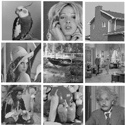
As mentioned earlier, the goal of the present research is to estimate the gamma value of an input image without any calibration information or knowledge of the imaging device in a local approach. Hence, a database of images with their related gamma values is initially needed to implement the algorithm. We used nine standard images shown in Figure 2, and applied twelve different gamma (from 0.2 to 2.4 interval o.2) to each of them to obtain twelve classes of images with different gamma (luminance) values.

Figure 2. Nine standard images used in the training stage of the proposed method, size of each image is 256×256.

   

2 2 2 2

A sliding window of size 64×64 is moved on the image from top-left side to bottom-right by sixteen pixels in each movement. A value of 64×64 pixels is chosen mainly because this value gives the best trade off between the rendering of local details and the need for reducing space dimensionality. Then nine aforementioned features are computed from each window. These features describe the image content. Hence a feature vector and a gamma value (0.2 to 2.4) will be available for each window. The final database contains 169 feature vectors for each image and a total of 18252 feature vectors for all nine training images. These features with the known gamma values are given to SVM for training.

To determine the gamma values of a new image, as mentioned earlier a sliding window of size 64×64 is moved on the image from top-left side to bottom-right by sixteen pixels in each movement. Then the same features are computed from each window and, SVM is employed to estimate the gamma value in each window.These features are fed to SVM to estimate the appropriate gamma value for each window.

Because of overlapping windows, some pixels have different gamma values. So the gamma value for each pixel is the average of gamma values of that pixel. Hence each pixel has its own gamma value. In other words, a matrix M of gamma values with the same size as the image is achieved. To enhance the image, according to Equation 2 the gamma values are applied to each pixel. Figure 3 shows the result. As it is shown in Figure 3(b), this approach has blocking effects on the image.

(a) Original image (b) gamma corrected image

Figure 3. Blocking effect in gamma correction.

In this step, to eliminate the blocking effects, first we apply average filter on M containing the gamma values. Then the filtered gamma values are applied to the image for gamma correction. Figure 4 is shown this result. As is clear the blocking effects are eliminated.

Figure 4.Image enhancement by our proposed method without the problem of blocking effect as exists in Figure 3(b).

6. EXPERIMENTAL RESULTS

In this paper we present a technique for estimating the gamma values without any calibration information or knowledge of the imaging device. We consider subjective and objective image quality assessment to demonstrate the performance of the proposed algorithm. We also compare the results of our proposed method with those generated by two other existing methods [3, 5] (see Figures 5 to 8). Subjective assessment in these figures indicates that proposed method estimates the gamma value more accurately for most of the input images.

Figures 5 to 8 (a) are outdoor images with high contrast under sunlight. Figures 5 to 8 (b) illustrate the results of the proposed method which bring out much more details that would be lost in dark areas of very high contrast in original images. None of the methods presented in [3, 5] does not have these capabilities. Figures 6 and 8 are images with unbalance illumination.

(a) Original image (b) Proposed method

(c) Method proposed in [3] (d) Method proposed in [5]

Figure 5. Comparison between the proposed method and the methods proposed in [3] and [5] (subjective quality assessment).

.

(a) Original image (b) Proposed method

(c) Method proposed in [3] (d) Method proposed in [5]

Figure 6. Comparison between the proposed method and the methods proposed in [3] and [5] (subjective quality assessment).

(a) Original image (b) Proposed method

(c) Method proposed in [3] (d) Method proposed in [5]

Figure 7. Comparison between the proposed method and the methods proposed in [3] and [5] (subjective quality assessment).

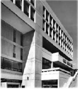
(a) Original image (b) Proposed method

(c) Method proposed in [3] (d) Method proposed in [5]

Although, this technique can be applied to color images. The HSV color model is adopted in processing color images [33]. In practice, the value (V) is only processed with the proposed method. Then the HVS color model with the modified V is transformed into the RGB color model. Figures 9 and 10 are shown two results of color images.

(a) Original image (b) Proposed method

Figure 9. Image enhancement for color image (subjective quality assessment).

(a) Original image (b) Proposed method

Figure 10. Image enhancement for color image (subjective quality assessment).

Numerical assessment is also performed to show the performance of the proposed method. SSIM is an example of the full reference numerical image quality assessment. Since the reference versions of above test images are not available, ten standard Matlab images are used. First, quality of these images has been damaged by different gamma values, then these images are applied to three algorithm to be restored. The scores listed in Table 1 are computed by SSIM over these ten images. The first row indicates SSIM values averaged over ten images. Respectively, the

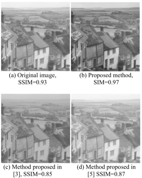
remaining rows represent standard deviation, minimum and maximum SSIM values of these ten images. As it is shown in Table 1, the SSIM provides higher scores to the proposed algorithm. The proposed algorithm outperforms the other two algorithms according to their SSIM. These scores are also in agreement with subjective evaluations of human observers. It is expected because this metric considers human visual perception factors. Figures 11 and 12 are two samples of the ten images with their SSIM values.

TABLE 1. SSIM values over ten independent images.

SSIM

values Proposed method proposed in [3]Method proposed in [5]Method

Mean 0.95 0.81 0.88

Std. dev. 0.04 0.1 0.09

Min 0.85 0.62 0.69

Max 0.98 0.94 0.97

(a) Original image,

SSIM=0.93 (b) Proposed method, SIM=0.97

(c) Method proposed in

[3], SSIM=0.85 (d) Method proposed in [5] SSIM=0.87

(a) Original image,

SSIM=0.82 (b) Proposed method, SSIM=0.96

(c) Method proposed in

[3], SSIM=0.68 (d) Method proposed in [5], SSIM=0.91

Figure 12. Comparison between the proposed method and the methods proposed in [3] and [5] (objective quality assessment).

7. CONCLUSIONS

We have introduced a new gamma correction method that estimates image gamma values without any calibration information or knowledge of the imaging device. The method is able to estimate appropriate gamma values for different regions of the image using SVM classifier. Experimental results in this research indicate that the proposed method improves image quality, and enhances the dynamic and details of the image.

8. REFERENCES

1. Pizurica, A. and Philips, W., “Estimating the probability of the presence of a signal of interest in multiresolution single and multiband image denoising”, IEEE Trans. Image Process, (2006), 654–665.

2. Nam, M. Y. and Rhee, P. K., “An efficient face recognition for variant illumination condition,”in proc. ISPACS, (2004), 111-115.

3. Shi, Y., Yang, J. and Wu, R., "Reducing Illumination Based on Nonlinear Gamma Correction," In Proc.

ICIP, San Antonio,(2007), 529-539.

4. Gonzalez, R. C. and Woods, R. E., Digital Image Processing. Prentice Hall, Upper Saddle River, NJ 07458, (2002).

5. Farid, H., "Blind inverse gamma correction", IEEE Transactions on Image Processing, Vol. 10, (2001),

pp. 1428-1433.

6. Lee, S., “Content-based image enhancement in the compressed domain based on multi-scale a-rooting algorithm”, Pattern Recognition Letters, Vol. 27 (2006), 1054–1066.

7. Pizer, S. M., E.P. Ambum and J.D. Austin, “Adaptive histogram equalization and its variation”, Computer Vision, Graphics, and Image ProcessingVol. 39, No. 3, (1987), 355–368.

8. Chen, S. D. and Ramli, A. R., “Minimum mean brightness error bihistogram equalization in contrast enhancement”, IEEE Transactions on Consumer Electronics, Vol.49, No. 4, (2003), 1310–1319. 9. FarshbafDoustar, M. and Hassanpour, H., "A

Locally-Adaptive Approach For Image Gamma Correction," 10th International Conference on Information Sciences,

Signal Processing and their Applications (ISSPA2010)

, (2010), 73-76.

10. Asadi Amiri, S., Hassanpour ,H. and Pouyan, A.,“Texture Based Image Enhancement Using Gamma Correction”, Middle-East Journal of Scientific Research, Vol. 6, (2010), 569-574.

11. Yi, D. and Lee, S., “Fourth-order partial differential equations for image enhancement”, Applied

Mathematics and Computation, Vol.175, No. 1,

(2006), 430–440.

12. Gilboa, G., Sochen, N. and Zeevi, Y. Y., “Image enhancement and denoising by complex diffusion processes”, IEEE Transactions on Pattern Analysis and Machine Intelligence , Vol. 26, No. 8, (2004),

1020–1036.

13. Sapiro, G.and Caselles, V., “Contrast enhancement via image evolution flows”, Graphical Models and Image Processing, Vol. 59, No. 6, (1997), 407–416.

14. Jobson, D. J., Rahman, Z. and Woodell G. A., “A multiscale Retinex for bridging the gap between color images and the human observation of scenes”, IEEE Transactions on Image Processing , Vol. 6, No. 7,

(1997), 965–976.

15. Kimmel, R., Elad, M., Shaked, D., Keshet, R. and Sobel I., “A variational framework for Retinex”, International Journal of Computer Vision, Vol. 52, No. 1, (2003), 7–

23.

16. Polesel, A., Ramponi, G. and Mathews, V. J., “Image enhancement via adaptive unsharp masking”, IEEE Transactions on Image Processing, Vol.9, No. 3,

(2000), 505–510.

17. Guillon, S., Baylou, P., Najim, M. and Keskes, N., “Adaptive nonlinear filters for 2D a nd 3D image enhancement”, Signal Processing, Vol. 67, No. 3 (1998), 237–254.

18. Fries, R. and Modestino, J., “Image enhancement by stochastic homomorphic filtering”, “IEEE Transactions on Acoustics, Speech, and Signal Processing, Vol. 27, No. 6, (1979), 625–637.

considerations on color image enhancement using homomorphic filtering”, Journal of Electronic Imaging

, Vol.6, No. 1, (1997), 108–113.

20. Gastaldo, P. and Zunino, R., Ingrid Heynderickx, Elena Vicario, “Objective quality assessment of displayed images by using neural networks”, Signal Processing Image Communication, (2005), 643–661.

21. Gadelmawla, E. S., “A vision system for surface roughness characterization using the gray level co-occurrence matrix”, NDT&E International , Vol.37 (2004), 577–588

22. Park, B. and Chen, Y. R., “Co-occurrence Matrix Texture Features of Multi-spectral Images on Poultry Carcasses“,Automation and Emerging Technologies, Vol.78, No.2, (2001), 127-139,

23. Haralick, R. M., Shanmugan, K. and Dinstein, I., “Textural features for image classification”, IEEE Trans. SMC, Vol. 3, (1973), 610–621.

24. Bonnel, J., Khademi, A., Krishnan, S. and Ioana, C., “Small bowe l image classification using cross -co-occurrence matrices on wavelet domain”, Biomedical Signal Processing and Control, Vol. 4, (2009), 7–15.

25. Rao, K. and Yip, P., “Discrete Cosine Transform: algorithms”, advantages, applications. Academic Press,

USA, (1990).

26. Al-Haj, A., “Combined DWT-DCT Digital Image

Watermarking”,Journal of Computer Science,Vol.3,

No. 9, (2007), 740-746.

27. Cristianini, N. and Shawe-Taylor, J., “Support Vector Machines,” Cambridge University Press, (2000). 28. DeCoste, D. and Schölkopf, B., “Training invariant

support vector machines”,Machine Learning, Vol.46,

No.(1/3), (2002).

29. El-Naqa, I., Yang, Y., Wernick, M., Galatsanos, N. and Nishikawa, N., “A Support Vector Machine Approach for Detection of Microcalcifications”, IEEE

TRANSACTIONS ON MEDICAL IMAGING, VOL.

21, NO. 12, (2002).

30. Scholkopf, B., Burges, C.,and Smola, A., “Advances in Kernel Methods: Support Vector Learning”, MA: MIT Press, Cambridge, (1999).

31. Wang, Z. and Bovik, A. C.,”Modern Image Quality Assessment”, Morgan and Claypool Publishing Company, New York, (2006).

32. Wang, Z., Bovik, A. C., Sheikh, H. R. and Simoncelli, E. P., "Image quality assessment: From error visibility to structural similarity" IEEE Transactios on Image Processing, Vol. 13, No. 4, (2002), 600-612.

33. Chen, Q., Xu, X., Sun, Q. and Xia, D: “A solution to the deficiencies of image enhancement”, Signal Processing,