NUMERICAL SOLUTION OF PRICING OF EUROPEAN PUT
OPTION WITH STOCHASTIC VOLITILITY
U.S. Rana*and A. Ahmad
Department of Mathematics, D.A.V. (P.G.) College Dehradun, Uttarakhnd, (248001), India drusrana@yahoo.co.in - asadahmad1004@yahoo.com
*Corresponding Author
(Received: December 13, 2009 – Accepted in Revised Form: April 23, 2011)
Abstract In this paper, European option pricing with stochastic volatility forecasted by well known GARCH model is discussed in context of Indian financial market. The data of Reliance Ltd. stock price from 3/01/2000 to 30/03/2009 is used and resulting partial differential equation is solved by Crank-Nicolson finite difference method for various interest rates and maturity in time. The sensitivity measures “Greeks” are also determined to validate the model. It is observed that the value of European put option increases with maturity time and decreases with interest rate.
Keywords European Option, Finite Difference Method, Stochastic Volatility, GARCH (1, 1), Greeks
هﺪﯿﮑﭼ
فوﺮﻌﻣلﺪﻣ ﻂﺳﻮﺗﯽﻓدﺎﺼﺗ تاﺮﯿﯿﻐﺗزاهدﺎﻔﺘﺳاﺎﺑﯽﯾﺎﭘورايراﺬﮔﺖﻤﯿﻗﻪﻟﺎﻘﻣﻦﯾارد GARCH
رد
ﺖﺳا هﺪﺷ ﯽﻨﯿﺑ ﺶﯿﭘ ﺪﻨﻫ ﯽﻟﺎﻣ رازﺎﺑ
.
ﺖﮐﺮﺷ مﺎﻬﺳ ﺖﻤﯿﻗ يﺎﻫ هداد زا ﻪﻟﺎﻘﻣ ﻦﯾا رد Reliance
ﺦﯾرﺎﺗ زا
3/ 1/ 2002
ﺎﺗ
30 /3 / 2009
دوﺪﺤﻣفﻼﺘﺧاشورﻂﺳﻮﺗﻞﺻﺎﺣﯽﺋﺰﺟﻞﯿﺴﻧاﺮﻔﯾدﻪﻟدﺎﻌﻣوهﺪﺷهدﺎﻔﺘﺳا Crank
-Nicolson ﺖﺳاهﺪﺷﻞﺣﺪﯿﺳرﺮﺳنﺎﻣزوﺮﯿﻐﺘﻣيﺎﻫدﻮﺳخﺮﻧياﺮﺑ
.
ﺖﯿﺳﺎﺴﺣناﺰﯿﻣ “Greeks”
رﻮﻈﻨﻣﻪﺑﺰﯿﻧ
ﺪﻧاهﺪﺷﺺﺨﺸﻣلﺪﻣ ﺪﯿﯾﺎﺗ
.
ﯽﯾﺎﭘورامﺎﻬﺳشزراﻪﮐﺖﺳاهﺪﺷهﺪﻫﺎﺸﻣ دﻮﺳخﺮﻧﺎﺑوﺶﯾاﺰﻓاﺪﯿﺳرﺮﺳناﺰﯿﻣﺎﺑ
ﺖﺳاﻪﺘﻓﺎﯾﺶﻫﺎﮐ
.
1. INTRODUCTION
It is widely acknowledged by financial researchers Black, et al [1], Merton [2] that the valuation of options leads to mathematical model which has long been an intriguing problem in different ways. The most fundamental input into an option pricing model is volatility, a measure of how much the underlying asset price is likely to vary over time. In financial markets, volatility presents a strange paradox to the market participants, academicians and policy makers Nelson [3],even volatility estimation is by no means an exact science but a lot of efforts have been expended in improving volatility model since better forecasts transforms into better pricing of option Bollerslev, et al [4], and Loudon, et al [5].
Recently, Loudon, et al [5], Mc-Millan, et al [6], Yu [7], Klaassen [8], Vilasuso [9] and Balaban [10] investigated the forecasting models in various markets and found that ARCH class of models
provide better forecast in terms of statistical error and evidence in favor of GARCH model over shorter intervals. In all these studies, various methods for the estimation of volatility and their performances were discussed in terms of statistical error but none of them used volatility forecasting in the valuation of option pricing governed by Black-Scholes partial differential equation.
consistent with observed option prices. One possible remedy for this is to make the volatility to be a function of time and strike price, which leads to a model in terms of parabolic partial differential equation in two variables i.e. volatility and underlying asset value.
In this paper an alternative approach is developed for the pricing of option by Black-Scholes partial differential equation regarding variable volatility which is forecasted by GARCH (1, 1) method and the resulting one dimensional parabolic partial differential equation is solved by implicit finite difference method [18].
2. FORMULATION AND SOLUTION OF MODEL
In the modeling of option pricing, the physical system is the financial market place and the particular object of observation is the price of the option’s underlying asset. In order to develop a model tractable by mathematical and computational techniques, it is assumed that price of European option
V
is a function of current value of the underlying asset ‘S
’ and the timet
i.e. V =V S t( , ). The continuous-time, Black-Scholes model to European option is[ ] [ ]
22 2 2 1
0 0, , 0,
2
V V V
rS S rV t T S
t S σ S
∂ + ∂ + ∂ − = ∈ ∈ ∞
∂ ∂ ∂
(1) where, T is time of expiration,ris a risk-free interest rate and
σ
is volatility of stock returns. Suppose K andS
T be strike price and price of underlying asset on the date of expiration T, respectively. In case ofS
T<
K
, it has a financial sense (in-the-money for holder of put option) and encourage to the holder of put option for exercise, because holder can sell the asset of worthS
Tat the cost of K. Thus, the gain of holder from the call option is(
K
−
S
T)
. In case ofS
T≥
K
, the holder will forfeit the right to exercise the option because he can buy the asset at a cost, less than or equal to predetermined strike price K. Similarly, in-the-money position for put option it isS
T<
K
, underwhich, asset is sold at higher price of K instead of
T
S
. Thus, the terminal payoffs from the long position in a European call and put options are defined as:( , ) max{ , 0}
V S T = K−S (2)
In put options, the terminal payoffs are non-negative, which reflect the vary nature of the options. This condition is defined at a future point in time and we wish to determine values backwards to an earlier point in time.
The option pricing problem (1) is posed on the domain
[
0,∞ ×] [
0,T]
with final condition (2). To complete the option pricing model, we prescribe two spatial boundary conditions atS
=
0
andS
= ∞
. But, in case of numerical solution, infinite grids cannot be represented in the computer so we truncate the solution domain artificially at pointmax
S
=
S
and replace the deleted portions with boundary conditions that minimize the deleterious effects of the truncation. The truncation pointS
max has to be sufficiently far from the region of interest in order to avoid the excessive error due to truncation and even if the imposed boundary conditions are imperfect, it does not materially affect the solution. On the other hand, unnecessarily large value ofS
max increases the computational cost. The choice ofS
max is consider in [19]. Hence, the solution value for the option pricing model (1) is[
0 ,Sm ax] [
× 0 ,T]
.Boundary conditions for put option are as:
• When
S
=
0
for some (t<T),S
will stay at zero at all subsequent times so that the option is sure to expire in-the-money. Hence( ) max
(0, ) r t T
V t =Ke− − −S (3)
• When
S
=
S
max, it becomes almost certain that the put value will be in out-of-the– money. Hencemax
(
, )
0
V S
t
=
(4)realistic than Black-Scholes model with constant volatility. Thus, volatility is an important issue to be addressed properly. From computational point of view, it is convenient to handle the pricing problem by forecasting the valuation by well known GARCH method than regarding volatility as function of strike price and time. Now we discuss the GARCH model.
2.1. GARCH (1, 1) Model
In 1986, Bollerslev [4] proposed GARCH (1, 1) model ast t t
y
=
ε σ
(5)with conditional variance σt2 =α α0+ iyt2−1+β σi t2−1 with
0 0, and 1, 1 0,
α > α β ≥ (6)
Where σt2, σt2−1 are volatilities on the day
t
and previous day, yt−1 is return on the previous day andt
ε
denotes a real-valued discrete-time stochastic process asε
t≈
N
(0,
σ
t2)
,y
t is the dependent variable of returnx
t at a timet
and α0,1 and 1
α β are weighted assigned to conditional and unconditional variances. The GARCH (1,1) regression model is obtained by assuming the
ε
ts be innovation in a linear regressiont t t
y
=
bx
+
ε
(7)The GARCH (1,1) process as defined in Equations 5 and 6 is stationary with
E y
( )
t=
0
,0 1 1
var( )
1
ty
α
α β
=
− −
andcov( , ) 0
y y
t s=
for t s
≠
if and only if
α β
1+ <
11
or characteristic roots of GARCH (1,1) process are outside the unit circle. The likelihood function for estimation of parameters is defined as:2 2
2 1
1
ln(2 )
ln(
)
2
T t t t ty
T
θ
π
σ
σ
=
= −
+
+
∑
l
(8)2.2. Discretization of Equation
For numerical solution of partial differential Equation 1 the rectangular domain[
0,Smax] [ ]
× 0,T is divided into (N+ ×1) (M +1) uniform grid points. The step width∆
S
and∆
t
are in general independent, wheremax 1
0
; 0,1, 2,...
i i
S
S S S i M
M
+ − = ∆ = − =
1 ; 0,1, 2,...
i i
T
t t t j N
N
+ − = ∆ = =
and Vi j, denotes the numerical approximation of
( , )
V i S j t∆ ∆ i.e. at value of V grid point ( , )i j . Keeping view for stability of finite difference scheme in mind, we used Crank and Nicolson (1947) method, which incorporates both explicit and implicit features [20]. The Crank-Nicolson scheme for Equation 1 is
1 1 1 1
1 1 1
i i i i i i
j j j j j j
aV − +bV +cV + =xV +− +yV+ +zV++ (9) where
(
)
(
)
(
)
(
)
2 2
2 2 2 2
2 2
2 2 2 2
1 1
1
4 2 2 4
1 1
1
4 2 2 4
i t r t
a ri i t b c ri i t
i t r t
x i ri t y z ri i t
σ σ σ σ σ σ ∆ ∆ = − ∆ = + + =− + ∆ ∆ ∆ = − ∆ = − − = + ∆
2.3. Discretization of Boundary and Initial
Conditions
We need the discretization of boundary and initial conditions for the European option. For a put option, boundary conditions are0
0 0,1, 2,...
M
j j
V =K and V = for j= N
and initial condition is:
(
)
max ,0 0,1,2,....
i N
V = K i S− ∆ for i= M
2.4. Stability of Scheme
It is unconditionally stable and the amplification factor of Crank-Nicolson scheme for Equation 1 is:2 2 2 2 2
2 1
1 (1 cos )
2 2
( ) 1
1 (1 cos )
which satisfies the von-Neumann stability condition G( )β ≤1 ; 0≤ ≤β π for any choice of
t
∆ and ∆S where β λ= ∆S and λ is wave number. But the choice of large value for
∆
t
leads to some undesirable results. Despite this, the main appeal of the method is its second order accuracy and stability which are achieved with minor increase in computational cost compared with the implicit method. Crank-Nikolson scheme ultimately reduced to a sparse system of algebraic equation, whose matrix form is1
[ ]{ }A V j =[X V]{ }j+ (10) where
0 0 ... 0 0 0 ... 0 0
0 ... 0 0
[ ] ... ... ... ... ... ... ... ... ... ... ... ... ... ...
0 0 0 0
0 0 0 0 0
b c
a b c
a b c
A
a b c
a b = and
0 0 ... 0 0 0 ... 0 0
0 ... 0 0
[ ] ... ... ... ... ... ... ... ... ... ... ... ... ... ...
0 0 0 0
0 0 0 0 0
y z
x y z
x y z
X
x y z
x y =
and { }f j+1, { }f j are known and unknown vectors respectively. It is a tridiagonal system and for its efficient numerical computation, well known Thomas algorithm is suggested [21]. The algorithm is an efficient implementation of the Gaussian elimination procedure and is numerically stableif aj<0,cj<0and bj> aj + cj . Fortunately,
these conditions are fulfilled by the tridiagonal system [21].
2.5.
Sensitivities
by Finite Difference Scheme
Finite difference method provides the price of anoption price at each (N+ ×1) (M+1) grids of the domain, which have a mathematical relevance and importance itself in financial aspects, the (N+1) th column is sufficient to determine the option price. But, it does not mean that the remaining values are useless, it is also significantly important in the determination of sensitivity parameters i.e.“Greeks”, directly on grid without having to go through the lengthy procedure. Since a finite difference scheme provide approximation for the derivatives with respect to
S
andt
at each time step. We can calculate the delta ( )∆ , gamma ( )Γ and theta ( )θ using values of associated grids as:2
( ) ( )
( ) ,
( ) 2 ( ) ( )
( ) ,
( ) ( )
( )
V S S V S
Delta
S
V S S V S V S S
Gamma
S
V t t V t
Theta t δ δ δ δ δ δ θ δ + − ∆ = + − + − Γ = + − =
3. RESULTS AND DISCUSSION
In this section, the parameters of GARCH (1,1) model for Reliance Ltd. areestimated as
0 1
0.0015801, 9.3498 005, 0.61598
t e
ε = α = − α = and
1 0.35168
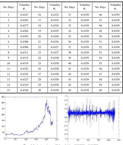
β = and used in Equations 5 and 6 for forecasting the volatility. The volatility of Reliance Ltd. is represented through Table 1 which shows a constant volatility after 30 days. Figure 1 represents the stock price and percentage change of stock return from 3/01/2000 to 30/03/2009 of Reliance Ltd. taking high price in a day. Option prices and sensitivity parameters for different stock pricesS, strike prices K =$30, 35, 40, 45, risk-free interest rate r = 8 %, 9 %, 10 %, 11 % at two different maturities are discussed through graphical and tabular forms. Table 2 shows the option prices for strike price K = $30,35,40,45 and interest rates r = 8 %, 9 %, 10 %, 11 % at different stock prices S with one month and two months maturity life of put option. Figures 2-5 show that the put price function is a decreasing function with respect to TABLE 1. 60 Days Forecasted Volatility of Reliance Ltd. using Parameters of GARCH (1,1) Model.
No. Days Volatility
i
σ
No. Days Volatilityi
σ
No. Days Volatilityi
σ
No. Days Volatilityi
σ
1 0.4247 16 0.4332 31 0.4339 46 0.4339
2 0.4262 17 0.4333 32 0.4339 47 0.4339
3 0.4277 18 0.4334 33 0.4339 48 0.4339
4 0.4284 19 0.4335 34 0.4339 49 0.4339
5 0.4293 20 0.4336 35 0.4339 50 0.4339
6 0.4300 21 0.4336 36 0.4339 51 0.4339
7 0.4306 22 0.4337 37 0.4339 52 0.4339
8 0.4311 23 0.4337 38 0.4339 53 0.4339
9 0.4315 24 0.4338 39 0.4339 54 0.4339
10 0.4319 25 0.4338 40 0.4339 55 0.4339
11 0.4322 26 0.4338 41 0.4339 56 0.4339
12 0.4325 27 0.4338 42 0.4339 57 0.4339
13 0.4327 28 0.4338 43 0.4339 58 0.4339
14 0.4319 29 0.4338 44 0.4339 59 0.4339
15 0.4330 30 0.4338 45 0.4339 60 0.4339
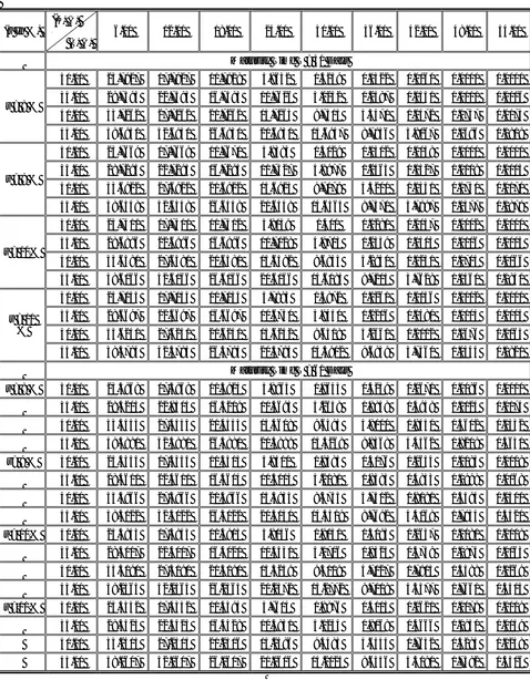
TABLE 2. Option Price for Different Stock Prices S, Strike Prices K = $30, $35, $40 and $45, Interest Rate r = 8 %, 9 %, 10 %, 11 % with One and Two Months Maturity Period.
(r In %) (K) ($)
(S) ($)
6.00 12.00 18.00 24.00 30.00 36.00 42.00 48.00 54.00
Maturity Time T = 30 Days
r = 8 %
30.00 23.7927 17.7927 11.7928 5.8632 1.4259 0.1322 0.0060 0.0000 0.0000
35.00 28.7595 22.7595 16.7595 10.7626 5.0242 1.2587 0.1551 0.0111 0.0006
40.00 33.7262 27.7262 21.7262 15.7263 9.7515 4.3471 1.1472 0.1757 0.0173
45.00 38.6930 32.6930 26.6930 20.6930 14.6947 8.7936 3.8167 1.0696 0.1909
r = 9 %
30.00 23.7669 17.7669 11.7670 5.8385 1.4129 0.1302 0.0058 0.0000 0.0000
35.00 28.7295 22.7295 16.7295 10.7327 4.9977 1.2463 0.1527 0.0108 0.0005
40.00 33.6922 27.6922 21.6922 15.6923 9.7179 4.3200 1.1351 0.1730 0.0170
45.00 38.6548 32.6548 26.6548 20.6548 14.6565 8.7570 3.7897 1.0577 0.1879
r = 10%
30.00 23.7411 17.7411 11.7412 5.8139 1.400 0.1281 0.0057 0.0002 0.0000
35.00 28.6996 22.6996 16.6996 10.7028 4.9713 1.2339 0.1503 0.0106 0.0005
40.00 33.6581 27.6581 21.6581 15.6582 9.6843 4.2930 1.1231 0.1703 0.0166
45.00 38.6166 32.6166 26.6166 20.6166 14.6184 8.7205 3.7628 1.0460 0.1850
r = 11 %
30.00 23.7153 17.7153 11.7154 5.7893 1.3872 0.1261 0.0056 0.0002 0.0000
35.00 28.6697 22.6697 16.6697 10.6730 4.9450 1.2216 0.1480 0.0104 0.0005
40.00 33.6241 27.6241 21.6241 15.6242 9.6508 4.2661 1.1112 0.1676 0.0163
45.00 38.5784 32.5784 26.5784 20.5784 14.5802 8.6839 3.7360 1.0344 0.1821
Maturity Time T = 60 Days
r = 8 % 30.00 23.5868 17.5868 11.5924 5.8965 1.9643 0.4259 0.0671 0.0086 0.0010
35.00 28.5205 22.8505 16.5209 10.5695 5.2658 1.8848 0.4948 0.1024 0.0174
40.00 33.4543 27.4543 21.4543 15.4608 9.6394 4.8000 1.8450 0.5602 0.1332
45.00 38.3881 32.3881 26.3881 20.3889 14.4268 8.8368 4.4562 1.8209 0.5631
r= 9 % 30.00 23.5355 17.5355 11.5413 5.8510 1.9385 0.4176 0.0654 0.0083 0.0009
35.00 28.4611 22.4611 16.4614 10.5113 5.2181 1.8585 0.4853 0.0998 0.0168
40.00 33.3866 27.3866 21.3866 15.3933 9.5755 4.7512 1.8181 0.5494 0.1300
45.00 38.3122 32.3122 26.3122 20.3130 14.3519 8.7692 4.4068 1.7934 0.5521
r= 10% 30.00 23.4843 17.4843 11.4903 5.8056 1.9130 0.4095 0.0637 0.0081 0.0009
35.00 28.4017 22.4017 16.4021 10.4531 5.1706 1.8325 0.4759 0.0974 0.0163
40.00 33.3190 27.3190 21.3190 15.3259 9.5119 4.7027 1.7915 0.5388 0.1269
45.00 38.2365 32.2364 26.2364 20.2372 14.2772 8.7018 4.3577 1.7661 0.5413
r =11% 30.00 23.4332 17.4332 11.4394 5.7604 1.8876 0.4015 0.0621 0.0078 0.0009
35.00 28.3424 22.3424 16.3428 10.3951 5.1234 1.8068 0.4666 0.0950 0.0159
40.00 33.2515 27.2515 21.2516 15.2586 9.4485 4.6544 1.7652 0.5283 0.1238
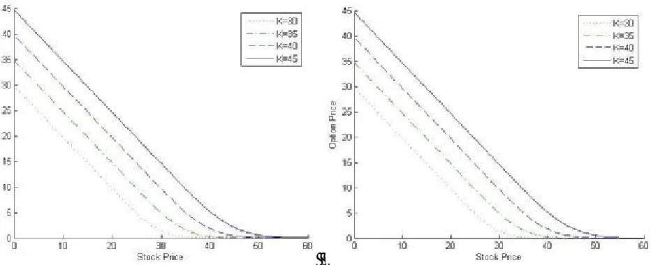
stock price (S) and present a concavity upward. The point S = K (i.e. at-the-money) the curve are more concave which referred that option lead to either in-the-money or out-of-the-money immediately. In case of in-the-money-(S<K) the value of option are changing in constant way with respect to the stock price (S) decrease, while the exponential change occurs when option become at-the-money as well as out-of-the money (Table 2, Figures 2-5).
The downward concavity conformed that a decrease in the asset price (S) will increase probability of a positive terminal payoff, resulting in a higher value of option. By keeping r small, t constant and increase of strike price from K = $30 to K = $45, the increment in option price has same trends with respect to stock price (S) and option is become in-the-money. But, as interest rate increases from = 8 % to r = 9 %, 10 % and 11 % the interval of positive terminal payoff reduces and
Figure 2. Option price for different stock prices S, strike prices K=$30, $35, $40, $45, interest rates r = 8 %, 9 % with one month maturity.
the option prices also reduce that means the possibility of positive terminal payoff decreases and portfolio become more sensitive with respect to interest rate increment, resulting a less option price. Hence, as the interest rate (r) increases, the option price decreases and the positive terminal payoff increase at only deep in-the-money. But, comparison of maturity life i.e. a short lived option with a long lived option depicts very strange results (Table 2). If option become deep
in-the-money, the option price decreases when maturity time increases, while in case of at-the-money and out-of the money option price increases with maturity time increase. Intuitively, in case of put option, probability of positive payoff increases as maturity time and interest rate increases.
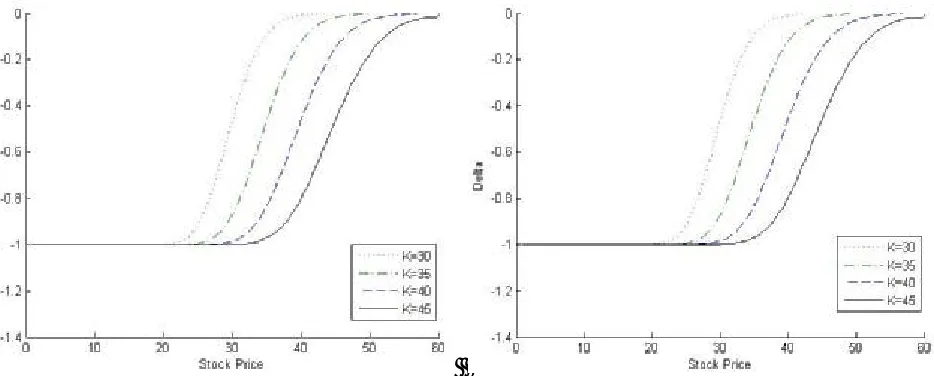
The delta (Δp) of put option shows the negative
values and lies (-1, 0). The negativity of delta (Δp)
for put option function confirmed the decreasing nature of the function with stock price (S) i.e. the
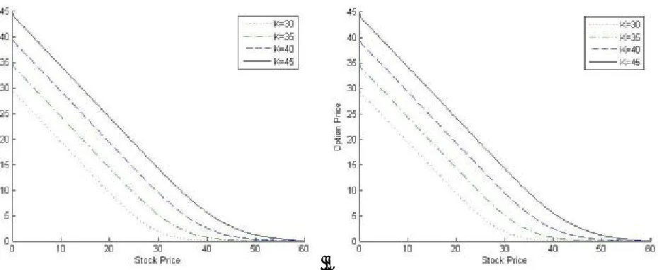
Figure 4. Option price for different stock prices S, strike prices K = $30, $35, $40, $45, interest rates r = 8 %, 9 % with two month maturity.
increment in the asset price causes a decrease in the value of put option prices and probability of a positive terminal payoff and then a long position for put option will be hedged by a continuously varying long position in the underlying asset. The effect of strike price is also significant to hedge to the portfolio. Figures 6-9 show the curves of delta (Δp) against stock price ( )S , change in
concavity appears where option is at-the-money
(S =K) so that the curve concave upward for in-the-money (0< <S K) and downward for out-of-the-money (K < < ∞S ).When option values become out-of-the-money ,the concavity increases as strike price (K) increases, which means the option price for a higher strike price (K) has a small changes in corresponding delta (Δp) i.e. the
delta (Δp) hedge dynamic for a higher strike price
(K) is less than as compared with low strike price
Figure 6. Delta (Δp) of the put option for different stock prices S, strike prices K = $30, $35, $40, $45,
interest rates r = 8 %, 9 % with one month maturity.
Figure 7. Delta (Δp) of the put option for different stock prices S, strike prices K = $30, $35, $40, $45,
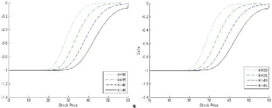
(K).The effect of interest rate on delta (Δp) also
represents an interesting result. It is observed that when strike price is sufficiently small (K=$30) the interest rate (r) has very small changes as r = 8 % to 9 %, 10 % and 11 % then the delta (Δp)
increases only when option become at-the-money, but it remains same for option being deep in-the-money and out-of-the-in-the-money. If we peer in the data of delta for K=$35, $40 and $45 for different interest rate, it has enough change with respect to
interest rate.
The impact of maturity life of option is countable in this problem as maturity life increases then the absolute values of delta decreases for each case of stock price, strike price and interest rate as result option is less sensitive i.e. increments in strike price, interest rate and maturity time increase the probability of positive terminal payoff increase. Further, the delta can be shown easily that
Figure 8. Delta (Δp) of the put option for different stock prices S, strike prices K=$30, $35, $40, $45,
interest rates r = 8 %, 9 % with two month maturity.
Figure 9. Delta(Δp) of the put option for different stock prices S, strike prices K = $30, $35, $40, $45,
li m t P 0
S
∂
→ ∞ =
∂ for all values of stock price (S).
While 0 1
lim 0
2 1
if S K
P
t if S K
S
if S K
>
∂
→ = − =
∂
− <
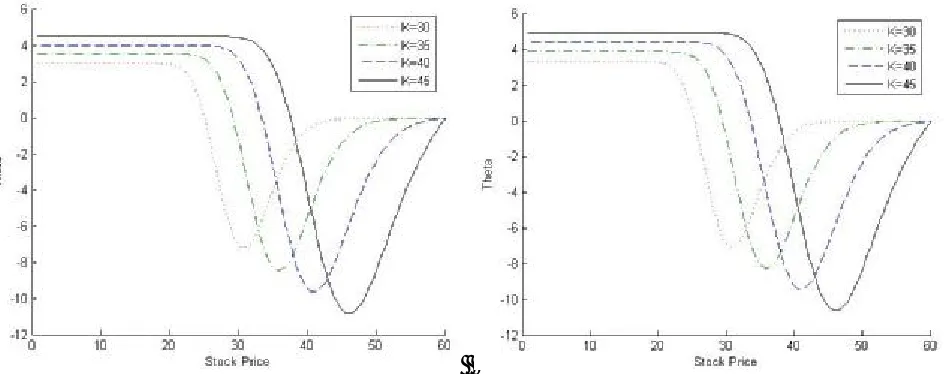
Figures 10-13 represent the values of theta (Δp) for a
put option against stock prices (S) are negative and positive. The curve of theta (Δp), tends
asymptotically as option become deep in-the-money. This means the results discussed above through Table 2 (i.e. the value of option decreases when option becomes out-of-the-money (S>K) and increases if option is in-the-money (S<K).While option becomesdeep in-the-money then the change in option price appears in a constant way) are validated from these figures. The negative sign of
Figure 10. Theta (Δp) of the put option for different stock prices S, strike prices K = $30, $35, $40, $45,
interest rates r = 8 %, 9 % with one month maturity.
Figure 11. Theta (Δp) of the put option for different stock prices S, strike prices K = $30, $35, $40, $45,
P t ∂
∂ confirms the long lived counterparts (Table 2). The positive sign of P
t ∂
∂ depicts the put values should be below their intrinsic values (K-S) and option should be grown to (K-S) at expiry. The tendency of asymptotic of curve also validatesthe change in option price, when option become deep in-the-money, constant way. It is also clear that the theta (θp)has its greatest absolute value when the
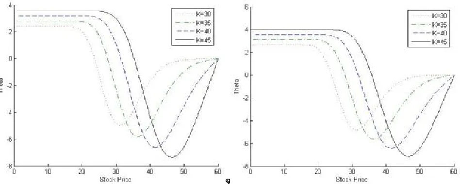
option is at-the-money (S<K) since the option may become in-the-money (S<K) or out-of-the-money (S>K) at an instant later. Also, the theta (θp) has a minimum absolute value when the option is sufficiently out-of-the-money (S>K). Hence, the absolute value of theta (θp) increases as strike price increases but decreases as interest rate (r) and maturity time increase (Figures 10-13).
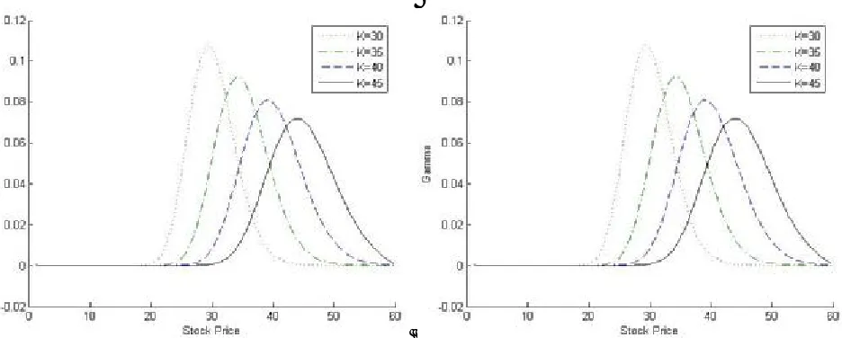
The gamma (γp) for put option are positive, this
Figure 12. Theta (Δp) of the put option for different stock prices S, strike prices K = $30, $35, $40, $45,
interest rates r = 8 %, 9 % with two month maturity.
Figure 13. Theta (Δp) of the put option for different stock prices S, strike prices K = $30, $35, $40, $45,
explain why the curves of the option price function with respect to stock price (S) are concave upward. From the figures, it is clear that, generally the absolute values of gamma are maximum as option become at-the-money (S=K) for each strike price (K), interest rate (r) and maturity time (T). This implies that the concavity of the curve for the option prices should be maximum as option become at-the-money (S=K) (Figures 2-6). The absolute values of
the gamma (γp)decreases as strike price increases i.e. the change of delta (Δp) is small when strike
price increases, this means a portfolio could be hedged by taking long position in put option. From Figures 14-17, it is clear that the gamma (γp) shows a bell shape curve which have a left long tail and right long tail when option becomes in-the-money (S<K) and out-of-the-in-the-money (S>K),
Figure 14. Gama (γp) of the put option for different stock prices S, strike prices K = $30, $35, $40, $45,
interest rates r = 8 % , 9 % with one month maturity.
Figure 15. Gama (γp) of the put option for different stock prices S, strike prices K = $30, $35, $40, $45,
respectively. From the figures of gammas (γp) it is quite clear that the area of left long tail is less than the area of right long tail. This means the changes of deltas (∆p) with respect to stock price (S) should be more dynamic when option becomes in-the-money whenever, option becomes out-of-the-money. This also shows that option has a positive terminal payoff in the case of in-the-money.
The results depict that the change of interest
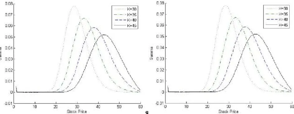
rate is insignificant on gamma values (Figures 14 and 15). But increase in the maturity time i.e. long lived option results in less values of gamma as compared to short lived option (Figures 14 and 16). So, the curvature of long lived option is less than short lived option, while the option prices for an option become at-the-money and out-of-the-money, long lived option are greater than short lived option which has a financial sense that hedging is less dynamic for long lived put option
Figure 16. Gama (γp) of the put option for different stock prices S, strike prices K = $30, $35, $40, $45,
interest rates r = 8 %, 9 % with two month maturity.
Figure 17. Gama (γp) of the put option for different stock prices S, strike prices K = $30, $35, $40, $45,
with short lived option.
4. CONCLUSION
Due to stochastic nature of financial market, the volatility is a crucial variable in option pricing and hedging strategies. The alternative approach for the stochastic volatility used in this paper form a one dimensional partial differential equation, where volatility is regarded as a function of stock price (S) and time (t), leads to a partial differential equation in two variables. From the computational point of view, the present model is more economic as compared to model with σ(S, t) The results may be useful for the financial engineers in order to understand the effect of stochastic volatility on the hedging movement.
5. REFERENCES
1. Black, F. and Scholes, M., “The Pricing of Options and Corporate Liabilities”, Journal of Political Economy, Vol .27, (1973), 637-659.
2. Merton, R.C., “Theory of Rational Option Pricing”, Journal of Economics and Management Science, Vol. 4, (1973), 141-183.
3. Nelson D.B., “Conditional Heteroskedasticity in Asset Returns: A New Approach”, Econometrica, Vol. 59, No. 2, (1991), 347-370.
4. Bollerslev, T.,“Generalized Autoregressive Conditional Heteroskedasticity”, Journal of Economerics, Vol. 31, (1986), 307-327.
5. Loudon, W, Watt, G. and Yadav, P., “An Empirical Analysis of Alternative Parametric ARCH Models”, Journal of Applied Econometrics, Vol. 15, (2000), 117-136.
6. Mc-Millan, D., Speight, A. and Gwilym, O., “Forecasting U.K. Stock Market Volatility”, Applied Financial Economics, Vol. 10, (2000), 435-448.
7. Yu, J., “Forecasting Volatility in the New Zealand Stock Market”, Appl. Fin. Economics, Vol. 12, (2002), 193-202.
8. Klassen, F., “Improving GARCH Volatility Forecasts”, Empirical Economics, Vol. 27, (2002), 363-394. 9. Vilasuso, J., “Forecasting Exchange Rate Volatility”,
Economic Letters, Vol. 76, (2002), 59-64.
10. Balban, E., “Comparative Forecasting Performance of Symmetric and Asymmetric Conditional Volatility Models of an Exchange Rate”, Economic Letters, Vol. 83, (2004), 99-105.
11. Hull, J. and White, A., “Valuing Derivative Securities using the Finite Difference Method”, J. Fin. and Quant. Analysis, Vol. 25, (1990), 88-99.
12. Avellaneda, M., Levy, A. and Paras, A., “Pricing and Hedging Derivative Securities in Markets with Uncertain Volatilities”, Appl. Math. Finance, Vol. 2, (1995), 73-88.
13. Avellaneda, M., Levy, A. and Paras, A., “Managing Security Risk of Portfolios of Derivatives: The Lagrangian Uncertain Volatility Model”, Appl. Math. Finance, Vol. 3, (1996), 21-52.
14. Chawla, M.M. and Evans, D.J., “High Accuracy Finite Difference Methods for the Valuation of Options”, Int. J. of Computer Mathematics, Vol. 82, (2005), 1157-1165.
15. Mayo, A., “High Order Accurate Implicit Finite Difference Method for Evaluating American Options”, The European Journal of Finance, Vol. 10, No. 3, (2004), 212-237.
16. Tangman, D.Y., Gopaul, A. and Bhurut, M., “Numerical Pricing of Options using High-Order Compact Finite Difference Schemes”, J. Comp. and Appl. Math., Vol. 218, No. 2, (2008), 270-280.
17. Hu, B.L.J. and Jiang, L., “Optimal Convergence Rate of the Explicit Finite Difference Scheme for American Option Valuation”, J. Comp. and Appl. Math., Vol. 230, No. 2, (2009), 583-599.
18. Rana, U.S., Kumar, N. and Baloni, J., “Mathematical Modeling for Homogeneous Tumor with Delay in Time”, International Journal of Engineering, Vol. 22, (2009), 49-56.
19. Ikonen, S. and Toivanen, J., “Pricing American Option using LU Decomposition”, Applied Mathematical Sciences, Vol. 1 (2007), 2529-2551.
20. Tavella, D. and Randall, C., “Pricing Financial Instrument: The Finite Difference Method”, John Wiley and Sons, Inc., New York, U.S.A., (2000).