Waterhammer Caused by Intermittent Pump Failure in Pipe Systems Including Parallel Pump Groups

Please cite this article as: A. Parsasadr, A. Ahmadi, A. Keramat, Waterhammer Caused by Intermittent Pump Failure in Pipe Systems Including Parallel Pump Groups, International Journal of Engineering (IJE), TRANSACTIONS A: Basics Vol. 29, No. 4, (April 2016) 444-453

International Journal of Engineering

Waterhammer Caused by Intermittent Pump Failure in Pipe Systems Including

Parallel Pump Groups

A. Parsasadra_{, A. Ahmadi}*a_{, A. Keramat}b

a _{Civil Engineering Department, Shahrood University of Technology, Shahrood, Iran} b _{Civil Engineering Department, Jundi Shapur University of Technology, Dezful, Iran}

P A P E R I N F O

Paper history:

Received 07 February 2016

Received in revised form 07 March 2016 Accepted 14 April 2016

Keywords:

Method of Characteristics Steady and Transient Flow Parallel Pumping System Pump Failure

Waterhammer

A B S T R A C T

The use of pumps linked in parallel or series in large scale pipe systems is usually inevitable, to meet the required head and discharge. Transient flow occurs following a pump failure in a pump group as a result of variations in the flow rate. This research is an investigation about waterhammer caused by one or more pump-switch off in a pump group when they are connected in parallel. The operation of each pump in the group during steady and unsteady state is analyzed. For this purpose, the fluid flow equations as well as the pumps relations including rotational speed change and head loss are combined and simultaneously solved in the time domain by the method of characteristic. From the results one can quantitatively conceive that the intermittent shut-down compared to suddenly switching off the whole pump group produces much less waterhammer pressures. Furthermore in the intermittent shut-down with different pump characteristics, it is suggested to firstly switch off the most powerful pump, and then the rest which are weaker. Appropriate interpretation about the transition results have been included.

doi: 10.5829/idosi.ije.2016.29.04a.02

1. INTRODUCTION1

In water supply systems, a fluid flow can be either steady or unsteady. An unsteady-state flow is a flow in which its characteristic changes by time. The unsteady flow occurs between two steady flows, hence it is usually called damping or transient flow. Waterhammer is a transient flow that happens following a sudden change in the flow rate such as closing the valves or sudden stop of a pump or turbine. The phenomenon depends on the principles and sudden changes in flow pressure as well as local and timing conditions of the flow movement. In some hydraulic systems such as water transition pipes, oil piping, distribution systems, water piping to turbines, water tunnels and pumping systems, a water hammer phenomena can cause quick waves in the system which in turn leads to pressure changes and structural movements of these vibrations in the axial and radial directions can cause considerable

1_{*Corresponding Author’s Email:[email protected] (A.} Ahmadi)

forces to be developed in the main pipe element or in the support systems.

Waterhammer can also cause high and low pressures in a pipe. The excessive pressures can cause damages to pumps, valves and other elements of the pipe system. Low pressures can also release dissolved air from the fluid that if it reaches to the vapor fluid pressure, it will intensifies the fluid vaporization, thus developing cavitations and extended damages.

The vibrations caused by waterhammer can also lead to significant damages. They are amplified when the pipeline or the contained flow is excited, with a frequency, approximately near the natural frequency of the system. In this condition, great stresses occur which endangers the whole system [1].

station. The pumps are connected together in parallel to provide required nodal discharges of the system. When a pumping group suddenly fails or some of the pumps are switched off due to lower water consumption, a waterhammer occurs. As a result, an investigation on pressure variations due to one or more pumps stop is very important for the design purposes. Many laboratory and theoretic studies have been performed on waterhammer, but in most of them, energy supply elements, e.g. the pumps and particularly the group of pumps subjected to waterhammer pressure have not been investigated. Meanwhile, the pump design, in terms of type, location, power, etc. plays a significant role in a safe and economic pump system.

Chaudhry [2] and Wylie [3] investigated transient flow in turbo machines with different forms of pump arrangement in a system by numerical models. Azhdary Moghaddam [4] examined unsteady flow and controlled it by surge tank and then proposed the equations for the highest and lowest water level in the tank. Afshar and Rohani [5] proposed a new implicit characteristic method for the transient flow computation in a system including a pump. Thorley [6] studied the operational safety of the system and Afsahar and Mahjoobi [7] studied optimal design of pumped pipeline systems for pressure decrease when a pump stops. Bergant [8, 9] and Keramat et al. [10] investigated the separation of water column in a pipeline due to a pump stop. Vazifeshenas et al. [11] examined the behavior of the flow in a mixed flow pump and the way cavitation phenomenon affected by different parameters. They found that the flow rate variation and pump revolution change had significant effect on cavitation phenomena. Ahmadi and Keramat [12] investigated fluid–structure interaction occurring due to junction coupling of a pump.

2. MATHEMATICAL MODEL

To model a pump station consisting parallel pump units during unsteady flow, hydraulic equations and pumps equations are simultaneously solved.

2. 1. Waterhammer Modeling To investigate a waterhammer event when a pump stops, two sets of equations: hydraulic flow differential equations (continuity and momentum equations) and pump relations have been used. Rough calculations between velocity and pressure change in a waterhammer can be made using the Joukowsky equation, and accurate computations are based on method of characteristic (MOC) [13].

2. 1. 1. Classic Water Hammer Theory Momentum and continuity equations are applied for the

computation of the unsteady pipe flow. The assumptions in the development of the equations are [14]:

(1) Flow in the pipeline is considered to be one-dimensional with the average velocity and uniform pressure at a section.

(2) Unsteady friction losses are approximated as quasi-steady state losses.

(3) The pipe section is full of water and remains full during the transient.

(4) There is no column separation during the transient event, i.e. the pressure is always greater than the liquid vapor pressure.

(5) Free gas content of the liquid is small such that the wave speed can be regarded as a constant.

(6) The pipe wall and the contained liquid behave linearly elastic.

(7) Structure-induced pressure changes are negligible compared to the classical waterhammer pressure in the liquid.

To investigate the flow in these conditions, the following momentum and continuity equations, Equations (1) and (2), are used:

2 0

H a Q

t gA x

 _  _

  (1)

0 2 Q Q

H Q

gA f

x t DA

 _ _{ }

  (2)

in which, t is time, g is acceleration of gravity, A is cross section of the flow, is velocity of wave transition in flow, x is distance, f is Darcy- Weisbach friction factor, D is inner diameter of the pipe ,Q is discharge and H is piezometric head.

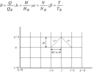
Since velocity and pressure in transient flow are the two dependent variables, and distance along the pipe (x) and time (t) are two independent variables, a system of two partial differential equations (hyperbolic) is achieved. The differential equations with partial derivatives (Equations (1), (2)) can be converted to two ordinary differential equations by means of the method of characteristic they are, then only valid on characteristic lines called . The waterhammer compatibility equations are written in the form of finite difference for a rectangular grid with the time marching indicated by index n and spatial discretization indicated by index i (Figure 1). Along the characteristic line

:

1

1

1 1 ₂ 2 1

n i

n n n n

i i i i

H

a a f x

H Q Q Q

gA gA gDA





  



 

 _ _{ } 

 

 _{  }

   

(3)

and along the characteristic line

_:

1

1

1 1 ₂ 2 1

n i

n n n n

i i i i

H

a a f x

H Q Q Q

gA gA gDA





  



 

 _ _{ } 

 

 

   

where Δx represents the reach length.

In the numerical solution, a steady state friction factor (f) which gives a constant value of the Darcy-Weisbach friction factor is incorporated. This assumption is satisfactory for slow transients where the wall shear stress has a quasi-steady behavior [15]. 2. 1. 1. 1. Reservoir Boundary Condition The pressure at the reservoir node is equal to the given head in the upstream and downstream boundary conditions. We also use the - relation in the upstream boundary and relation in the downstream boundary in the numerical computations based on the characteristic lines.

2. 1. 2. Pump Boundary Condition We use the pumps relationships to obtain the transient flow characteristics in pumps station. The pump characteristic curves in transient state are used to solve these equations.

2. 1. 2. 1. Pump Characteristic Curve in Transient State Two basic assumptions are made throughout the transient analysis of the pumps [3]. The first one is that the steady-state characteristic relation of pump is hold for unsteady-state situation. The other is the validity of the homologous relations.

The discharge, Q, of a centrifugal pump is a function of the rotational speed, N, and the pumping head, H, whereas the transient-state speed changes depending upon the net torque, T, and the combined moment of inertia of the rotating parts of the pump and motor and liquid entrained in the impeller. Thus, four variables, including Q, H, N and T are needed for the mathematical representation of a pump.

The curves showing the relationships between these variables are called the pump characteristics or pump performance curves. The values of Q, H, N,and T at the point of best efficiency are referred to as the rated conditions [16] and they are denoted by subscript R. Non-dimensional pump quantitative are then defined as:

; ; ;

R R R R

Q H N T

h

Q H N T

    ₍₅₎

Figure 1. Characteristic grid with specified time intervals

Pump characteristic or pump performance curves based on the signs of the two parameters and (the direction of the rotation of the pump impeller and the direction of the flow with respect to the steady state conditions) are divided into four working zones listed in Table 1 [3].

The pressure characteristic and net torque curves, for different values of the x angle are represented by WH

and WB parameters, respectively. They are often

provided for particular specific speeds (NS) e.g. 24.5,

147 and 261 (SI) [2, 3]. The following relations hold:

H _{2 2} B _{2 2}

1

0.5 0.75

h β

W , W

α α

x π tan α

R R

s R

N Q N

H

 

 

 

 

 



(6)

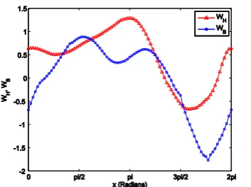
In the above equations, in order to determine the specific speeds in the SI unit, the unit of rotational speed, discharge and head are revolutions per minute, cubic meter per second and meter, respectively [3]. These curves being WH ,WB are respectively used for

head and torque determination in steady state (normal operation of pump) and also transient state (all four types of pump operation). They are specified in red and blue colors for the 24.5 unit specific speed in Figure 2.

The discharge values (Q) and rotational speed (N) are determined independently from the head balance equation and speed- change equation using the pump characteristic curves in transient state. Using the WH

curve we have:

1

tan ( ), ,

R R

Q N

x

Q N



  

 

    (7)

 

2 2 H

h

W x

   (8)

 





. .

H R

H W x   H (9)

and for the WB curve we will have:

 

2 2 WB x



   (10)

 





. .

B R

T W x   T (11)

TABLE 1. Four zones of pump operation

Turbine zone

Dissipation zone

Normal zone

Reversed speed dissipation zone

Figure 2. The pump characteristic curve (pressure-head and net rotation) in transient state for 24.5 unit specific speed

where the torque values in the rated condition are obtained from the following relation:

60 2

R R R

R R

H Q T

N 

 

 (12)

where and are respectively the specific weight of liquid and pump efficiency at the rated conditions. In the above equations, WH(x) and WB(x) values are

obtained using x from (Equation (7)), and is read from the pump characteristic curve (Figure 2).

2. 1. 2. 2. Pumps Governing Equations The group of pumps connected in parallel are examined in this study. In the system of pumps in parallel, the total discharge of system is equal to sum of discharges of all pump but in this condition

the overall head of the system is the same (

).

The pumps relations are (Equations (5)-(12)) used to obtain the discharge and rotational speed in the transient flow, and then the values of head and torque are obtained using characteristic curves of each pump. Each pump has two equations: head balance and speed-change. They are used in the transient flow condition for obtaining the flow rate and pressure head for the pump group.

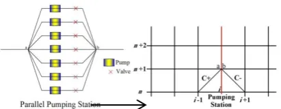
For simulation of a pumping station, a node is considered as the parallel pump group. This node is represented in Figure 3 (right), which contains two computational values at its either side due to the pumping action. As a result, for the sake of numerical modeling, the pump group with all of its apparatus and connected accessories are integrated in one point whose quantities are obtained at any time section by means of the hydraulic and pump relations.

2. 1. 2. 2. 1. Head Balance Equations in a Parallel Pumping Station The head balance equation can be applied both in transient and steady states. At steady state condition, the rotational speed is equal to the rated

condition because the pump is working with the normal rotational speed (αi =1). Accordingly, the head of i-th

pump (HPi) in the group is obtained with respect to (i

= 1, 2, …, NPu, NPu is the total number of pumps) being the dimensionless discharge parameter. But during the transient state, the speed-change equations of pumps are employed to obtain the flow characteristics in the pump boundary due to changes of rotational speed by time.

2. 1. 2. 2. 1.1. Head Balance Equations in Steady State: The steady state head and discharge are used as initial conditions of the transient state. To this aim, the energy relation between two points at the upstream and downstream is written as follows:

 





3 1 2 2

2 2

0 , 1, 2,...,

. .

. . 2

i

i i

i P f

P i i H i R

j System f

j j

FH H E E h i NPu

H W x H

f L Q h

gD A

 

     

 





 

(13)

In the above equations, E1 and E3 are energy at upstream

and downstream boundary of the system, respectively, and are length, diameter and cross-sectional area of the j-th pipe. As during the steady state condition, αi =1 the above relation can be simplified as

follows:





2

i i H i R 3 1 2 j System

2 j j

System 1 2

1

FH 1 .W x .H E E

f .L .Q 0 2gD A

NPu

NPu i

i

Q Q Q Q Q





   

 

   





(14)

where NPu is the number of pump connected in parallel. The above NPu equations have to be solved simultaneously for the unknown αi, νi, βi, hi (i=1, 2, …,

NPu). The above nonlinear equations (there is an equation for each pump in accordance with Equation (13)) must be solved simultaneously in a way, so then should be the same head for all pumps except for the need to making the FH value equal to zero. In other words, the head of each pump depends on the discharge passing through it, and the required energy to overcome the friction in the whole piping system is dependent on the discharge passing from total pumps.

2. 1. 2. 2. 1.2. Head Balance Equation in Transient State There is a head balance equation for each pump of the system of pumps in parallel.

If Ha and Hb are respectively the head before and

after the pumping station (Figure 4), then the head balance equation for the system of pumps connected in parallel at any time is as follows:

0 , 1, 2, , i i

a P f b

Figure 3. Parallel pumping station as a boundary condition in the computational grid.

where is local head loss at valve, after i-th pump and

HPi is head of i-th pump (the sum of this friction loss

and the pump head is the same for all pumps, Figure 3). To solve the transient flow caused by power failure, C+ and C- equations are used for points a and b, respectively (Figures 3 and 4). The head balance equation is finally simplified as follows for i-th pump during flow transients:









 





.

. . 0

i

i p m System p m

H i R i i

FH C C Q B B

W x H  

   

  

(16)

1 1 1

1 1 1

; ;

;

n n n

p i i p i

n n n

m i i m i

C H BQ B B R Q

C H BQ B B R Q

  

  

   

   

(17)

In Equations (15) and (16) the index is the pump number and in Equation (17) it shows the computational point in the grid being as pump station in the pipe system (Figure 3).

2. 1. 2. 2. 2. Torque Equation (Speed-change) in Parallel Pumping Station The change in the rotational speed of the pump depends on the unbalanced torque applied on each pump so that an equation is created for each pump [2, 3]:

2 . 60

d dN

T I I

dt dt

 

    (18)

in which I is the moment of inertia of rotor which include the pump and the contained liquid (combined polar moment of inertia of the pump, motor, shaft, and liquid entrained in the pump impeller). Throughly presents a graph of I (Kg.m2) for predicting the inertia of pump impellers, including the entrained water and shaft vs. a power coefficient (P/N3_{) in which P is the} shaft power in kilowatts supplied to the pump at rated condition, and N is the rotational speed in rpm. A linear regression analysis of logarithmic values of 284 data points from five pump manufacturers yields the

equation

_{ }

3 1.5 10 P P I N    _{ }  

. A similar study, by

Thorley, of 272 data points for motor rotational inertia yields the equation, ₁₁₈ 1.48

m P I N    _{ }  

. The total rotational

inertia is suitable to be used is the sum of the two,

P m

I I I [3]. and ω are the rotational speed in revolutions per minute and radians per second, respectively. Based on Equations (5) and (18) we have:

2 . . 60 R R R N T d I

T T dt

 

    (19)

Using Equation (19) and converse Equation (18) written in finite difference over time the torque equation (speed-change) for i-th pump is as follows:













. . 0,

15

1, 2, ,

i i R i i i i R i

R i

i i i i i

R i

T t I N

N I T t i NPu                       (20)

while the zero indexes in αi0 and βi0 represents their

values at the previous time step. Finally, the speed-change equation for the i-th pump in a parallel pump group reduces to:





 





2 2

0

1 .

. . 0

15. tan ( )

i i i i i

R i

i i i

R i

i i

i

FT W B x

N I T t x     _{ }              (21)

In this equation, is equal to the value of in x

point for i-th pump, given by Figure 2.

To solve the nonlinear Equations (16) and (21) simultaneously (making 2(Npu)) equations in total), the Newton-Raphson method is used [2, 3].

After solving the mentioned nonlinear equations simultaneously,ν1, ν2 … νNPu, α1, α2 … αNPu values (NPu is the total number of pumps) are obtained at each time step. Using Equations (22) and (25), one can calculate the discharge of the system, the rotational speed of the pump, the pump head and torque at each time step at each pump:

1 .

i

n

System i R

i

Q  Q







.

i i R

N  N (23)





 

i i

P i i H i R

H    W x H (24)





 

i i

P i i B i R

T    W x T (25)

3. NUMERICAL EXAMPLES AND DISCUSSION

), the diameter of first and second pipe have been considered the same and equal to 0.305 m ( ). The Darcy-Weisbach friction

factor for each pipe is equal to 0.01 ( ) and

the wave speed in the system is equal to 1098 m/s ( ). Assuming different parallel pump groups in the mentioned piping system, we will examine the waterhammer and its critical pressures due to power failure at different scenarios by numerical solution of relevant equations using Matlab software.

3. 1. Waterhammer Pressure versus Number of Pumps in Group Consider consumption fluctuations per day (governed by maximum hourly coefficient) as well as fluctuations in different days of a year (daily maximum coefficient), it is suggested to use multiple pumps in pumping station instead of using one pump to supply the required discharge. Doing so, when the consumption is high, all pumps in the group are employed to meet the demands and during lower demands some pumps are switched off. Two hypothetical pumps are used in the numerical simulation. Table 2 represents two different pump characteristics which their rotation speed is 1450 rpm in normal mode. Different pump groups made from one to twenty identical pumps (pump No.1 in Table 2) are used in the mentioned piping system. The obtained flow rate of the system in steady state for the variable pump groups are given in Figure 5. This figure shows that connection of pumps in parallel affects operating point of each pump. In other words, increasing the number of pumps does not increase the discharge up to a constant factor.

TABLE 2. Pumps characteristics

Pump No.2 Pump No.1

1450 1450

94.5 124.55

0.264 0.399

Rated efficiency 0.9 0.9

Figure 2. The passing discharge through the piping system versus the number of pumps (1 to 20) in the group at steady state condition.

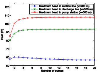
This means that there is an appropriate pump number in group which provides most efficient pressure. Figure 6 represents the impacts that are put at piping system at various points of maximum pressure head at the time of power failure to pump group.

Figure 6 shows the effect of the number of parallel pumps on the maximum pressure head in the suction line, discharge line and pump station, with changing the pumps number from one to twenty. As Figure 6 specifies, in the mentioned piping system the maximum pressure head occurs at the pumping system station in all cases of pump groups (compare the red graph with green and blue ones in Figure 6).

3. 2. Transients Caused by one More Pumps Failure in a Parallel Pump Group The waterhammer pressure rise in a parallel pump group (ΔP) will be lower when the pumps are switched off one by one compared to the time when it happens suddenly. The reason is that other pumps transmit the flow thus leading to less change of the flow rate (ΔV) and lower speed-changes and pressure increase according to Joukowsky’s relation ( - ).

3. 2. 1. The Switch off of the Two Different Pumps in Two Steps The shut-down of each of the pumps has different effects on the system, if the pump group of the piping system consists of two different pumps with different powers (pumps No.1 and 2 in Table 2).

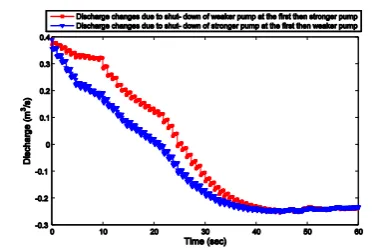
Figure 7 shows the pressure head caused by waterhammer in 300 meter before the pumping system, in other words 200 meter after the no.1 reservoir. Figure 8 shows the passing discharge through the system in transient state due to the shut-down of each of the pumps within 10 seconds from the previous pump.

In Figures 7 and 8 in the red graph first the weaker pump (pump no.1) and after 10 seconds the stronger pump switched off (pump no.2), and in the blue graph it is vice versa.

As seen in Figure 7, the critical pressures (maximum and minimum) in red and blue graphs are equal to 58.98 m and -10.96 m and 53.31 m and -9.03 m, respectively. In blue graph the maximum pressure head is 5.67 meters (10.64% reduction in the maximum pressure head) lesser and minimum pressure is 1.93 meters (21.37% increase of the minimum pressure head) higher than the red graph.

According to Figure 7, the blue graph (the strong pump failure occurs first, then weak pump) is superior to red one (the weak pump failure occurs first, then the strong pump) from the view point of the entered critical pressure head to the system.

Figure 8 illustrates the difference of pumps’ power and their shut down order on the flow rate changes.

Figure 7. The waterhammer pressure due to shut-down of each of the pumps with an interval of 10 seconds from the previous failure in the suction line (x=200 m) (red: shut- down of the weaker pump at first and then the stronger pump; blue: shut-down of the stronger pump at first and then the weaker pump).

Figure 8. the discharge changes in the piping system with respect to the time due to shut-down of each of the pumps with an interval of 10 seconds from the previous pump (red: the shut-down of weaker pump at first, then stronger pump; blue: the shut- own of stronger pump at first, then weaker pump)

So when the strong pump failure is occurred prior to its opposite mode, the discharge in piping system is decreased more quickly; this discharge reduction in both conditions is to the extent that the flow (t= 24.55 s in red graph and t= 20.9 s in blue graph) is stopped at a moment and then the flow will be forced run in the pipes in the opposite direction because of the gravity. 3. 2. 2. The Switch off of the Two Similar Pumps in Two Steps The similar and same pumps are mostly used for water pumping in the pumping systems because of the increase of the system efficiency at steady state condition. Because if the pumps are different then the weaker pump is less powerful to pass the flow and the head compared to the stronger one and that reduces the efficiency of the pump system. Now if the mentioned piping system consists of two similar pumps that are connected in parallel (pump no.1 from Table 2), while the switched off the pumps occurs in 10-second intervals from each other, the passing discharged through each pump and both pumps of time and the ratio of each pump rotation speed to the rated condition (α ) of time are in the forms of Figures 9 and 10, respectively.

As Figure 9 depicts as soon as one of the pumps fails, the flow is reduced quickly in the pump and is increased in the other pump. The flow reduction in the failed pump (first pump, red mode of Figure 9) is to the extent that in a very short time the passing discharge through it, becomes zero and then passes it in the opposite direction of water and this condition continues until the second pump is failed (black mode of Figure 9).

After the second pump is failed the passing discharge through the first pump quickly increases and the flow direction returns to normal, and the passing discharge through the second pump quickly reduces, these reductions and increases continues till the passing discharge through both pumps reaches equal value and after that, both bumps work quietly similar. The passing flow through both pumps (the passing flow through pipes) is reducing when the first pump is failed. Also the fractures on the discharge results are due to waterhammer wave in the system. On the other hand, this figure shows that the produced discharge in any of these parallel pumps is lower than the one which is produced in pumps that are placed on pump station singly, so when one of the pumps fails and exits from the pump station the pumps’ produced discharge will be increased.

the 10th second, and after its failure, the rotation speed of its impeller reduces and the first pump rotation speed increases. These reductions and increases continue till the rotation speed of both pumps reaches an equal value. Then, both pumps work quite similar (Figure 9). When the flow is stopped in pipes ( in Figure 9), the pumps’ impeller rotate in normal direction due to inertia of different rotating parts of pump (pump motor and its liquid), and after the flow is run oppositely in the pipes then the pump rotation speed decreases extremely, till reaches to zero ( in Figure 10) and then begins to rotate in the opposite direction.

Dissipation zone refers to the distance between the times when the flow discharge becomes zero until pump rotation speed becomes zero [21].

Figure 9. The discharge changes with respect to the time for each of the pumps in intermittent pump failure with an interval of 10 seconds (red: first pump is failed at zero time; black: second pump is failed in 10 seconds; blue: the total passing discharge through the pumps)

Figure 10. The changes versus time for each of the

pumps in intermittent pump failure with an interval of 10 seconds (red: first pump is failed at zero time; black: second pump is failed in 10 seconds)

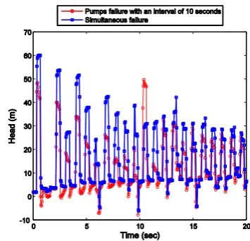
Figure11 represents the difference between two pumps intermittent shut down and simultaneous failure in the pressures caused by waterhammer in 300 meter before the pumping system which are pressurized a lot positively.

As Figure 11 shows, the two pumps intermittent failure (Figure 11, red graph) causes the maximum head to be reduced to 10.55 meters (21.26%) at this station of the piping system compared to simultaneous failure (Figure 11, blue graph).

3. 3. Power Failure of System of Pumps in Parallel If the pumping system consists of 6 similar pumps, and the pumping system fails suddenly, Figures 12 and 13 show the pressure in suction line (x=200 m) and discharge line (x=800 m), respectively.

Figure 11. The pressure head caused by waterhammer due to pumps intermittent and simultaneous failure with time step of 10 seconds (blue: simultaneous failure; red: pumps failure with an interval of 10 seconds)

Figure 13. The pressure head caused by waterhammer due to power failure of pump group in discharge line (x=800 m)

Comparing Figures 12 and 13, we can conclude that the waterhammer wave at time ( ) (L is the length of each pump) is returned to the pump station (suction line 0.91 seconds, discharge line 1.82 seconds), then causing the fracture in pressure results.

4. CONCLUSION

In this research we examined the system of pumps in parallel and waterhammer caused by its failure in intermittent (one after the other) and simultaneous failure. For this purpose, we used pumps relations and flow hydraulic equations. Then these equations were solved by method of characteristics. Finally the results were analyzed for each system separately, and the results were drawn in comparison to the critical pressures and stress history and system performance in transient state to reduce the effects of waterhammer in the system of pumps in parallel.

Examining studies on numerical model results which were presented for various states of parallel pump groups, we have concluded that in a parallel pump group with intermittent failure, lower pressures caused by waterhammer are put to different parts of system compared to simultaneous failure, and the stronger the pumping system, the more severity is the water hammer. So a solution to design the pumping and piping system for reducing the pressures caused by waterhammer is use of system of pumps in parallel with intermittent failure. Also the use of different pumps in parallel pumping system concludes to decrease in the maximum pressure in the system when the strong pump fails. When the strong pump fails, first causes lower pressures in the piping system compared to the state which the weak pump fails first, because the weak pump is working. Then the best way for pumps to be failed in system of pumps in parallel about maximum waterhammer pressure to the system, is their failure

based on their power order, because other working pumps cause the flow to be run in the system and therefore the speed change ( ) caused by pump failure is reduced. This would reduce the maximum pressure of the system. If the opposite happens, because the weak pump is working the pressure has lower fluctuations compared to the previous steady state condition, but when the strong pump fails the pressure in the system is much greater because there is no other working pump to reduce the fluctuations. This can be extended for waterhammer states caused by turning on the pumps (in reverse), thus it is better to turn on the weak pump first to make the waterhammer partial and then the stronger pump amplifies the flow by creating fewer waterhammer.

5. REFERENCES

1. Taebi, A. and Chamani, M., Urban water distribution networks. 2000, Isfahan University of Technology Press.

2. Chaudhry, M.H., Applied hydraulic transients. 1979, Springer. 3. Wylie, E.B., STEETER, V. and LISHENG, S., "Fluid transients

in systems prentice-hall", Englewood Cliffs, New Jersey, (1993).

4. Azhdari, M.M., "Analysis and design of a simple surge tank", (2004).

5. Afshar, M. and Rohani, M., "Water hammer simulation by implicit method of characteristic", International Journal of

Pressure vessels and piping, Vol. 85, No. 12, (2008), 851-859.

6. Thorley, A., "Fluid transients in pipeline systems–a guide to the control and suppression of fluids transients in liquids in closed conduits", Professional Engineering Publishing Limited,

United Kingdom, (2004).

7. Afshar, M. and Mahjoobi, J., "Optimal design of pumped pipeline systems using genetic algorithm and mathematical optimization", Journal of water & wastewater, (2008), 35-48. 8. Bergant, A. and Simpson, A.R., "Pipeline column separation

flow regimes", Journal of Hydraulic Engineering, Vol. 125, No. 8, (1999), 835-848.

9. Bergant, A., Simpson, A.R. and Tijsseling, A.S., "Water hammer with column separation: A historical review", Journal

of fluids and structures, Vol. 22, No. 2, (2006), 135-171.

10. Keramat, A., Ahmadi, A. and Majd, A., "Transient cavitating pipe flow due to a pump failure", in International meeting of the workgroup on cavitation and dynamic problems in hydraulic machinery and systems. (2009).

11. Vazifeshenas, Y., Farhadi, M., Sedighi, K. and Shafaghat, R., "Numerical simulation of cavitation in mixed flow pump", International Journal of Engineering-Transactions C:

Aspects, Vol. 28, No. 6, (2015), 956-964.

12. Ahmadi, A. and Keramat, A., "Investigation of fluid–structure interaction with various types of junction coupling", Journal of

fluids and structures, Vol. 26, No. 7, (2010), 1123-1141.

13. Shu, J.-J., "Modelling vaporous cavitation on fluid transients",

International Journal of Pressure vessels and piping, Vol. 80,

No. 3, (2003), 187-195.

15. Bergant, A., Ross Simpson, A. and Vìtkovsk, J., "Developments in unsteady pipe flow friction modelling", Journal of Hydraulic

Research, Vol. 39, No. 3, (2001), 249-257.

16. Stepanoff, A.J., "Centrifugal and axial flow pumps", (1948).

Waterhammer Caused by Intermittent Pump Failure in Pipe Systems Including

Parallel Pump Groups

A. Parsasadra_{, A. Ahmadi}a_{, A. Keramat}b

a _{Civil Engineering Department, Shahrood University of Technology, Shahrood, Iran} b _{Civil Engineering Department, Jundi Shapur University of Technology, Dezful, Iran}

P A P E R I N F O

Paper history:

Received 07 February 2016

Received in revised form 07 March 2016 Accepted 14 April 2016

Keywords:

Method of Characteristics Steady and Transient Flow Parallel Pumping System Pump Failure Waterhammer ديكچ س رد نتسی یاّ گرشب کی هات ِب رداق پوپ يی

بد ٍ ذّ ی ً درَه سای وً ی ذضاب پوپ اذل زس ترَص ِب ار اّ ی ای ساَه ی ِب زریذدکی ه لصته ی ذٌٌک ذّ ات یبد ٍ ً درَه سای هأت يی پوپ زگا لاح .ددزگ اّ

ی نتسیس صاپوپ ًاْگاً ترَص ِب ی

چَق ِبزض ،ذًَض فقَته

ه خر ی ذّر جَه ترَص ِب ِک اّ

ی راطف ی فٌه ٍ تبثه ی ه زّاظ ی دَض ا . يی جَه صٌت ىذهآ دَخَب ثعاب اّ اّ ی دسب رای س یدادی اشخا رد ی س نتسی ه ی .دَض ا رد يی قحت قی سرزب ِب ی ِبزض ی ضاً چَق ی ًاْگاً فقَت سا ی

ضَهاخ ٍ ی ماگ ٍ ىاهشوّ ماگ ِب اَدًا س نتسی ساَه صاپوپ ی ٌچوّ ٍ يی س سا پوپ زّ دزکلوع نتسی

راگذًاه تلاح رد صاپوپ راگذًاهزیغ ٍ

تسا ُذض ِتخادزپ .

ازب ی ا يدی

ّ سا لصاح تلاداعه رَظٌه کیلٍرذی

زخ ،ىای پوپ زب نکاح طباٍر َُحً ٍ اّ

ی پوپ لاصتا اب اّ زریذکی کزت ،بی ترَدص ِدب ٍ

زص ِصخطه طَطخ شٍر اب ىاهشوّ حی

ُذض لح ىاهس ُسَح رد اتً ِب ِخَت اب .ذًا

حی ضَهاخ ،ُذض لصاح ی ماگ ِب پوپ ماگ ادّ

اّراطف ِخَت لباق صّاک ثعاب ی

ضاً ی ِبزض سا ی س رد چَق نتسی ه ی دَض ضَهاخ تلاح رد . ی

مادگ ِدب پدوپ زدگا ،مادگ ادّ ی س نتسی ساَه صاپوپ ،ی تزت ،ذٌضاب تٍافته بی ضَهاخ ی زّ کی پوپ سا ثات اّ زی افته تٍ ی س ِب نتسی ه دراٍ ی ٍ ذٌک یده داٌْطیپ دَدض پوپ ِک ذًَض شَهاخ ىاطترذق بیتزت ِب اّ ا

يی اتً ساسا زب زها حی

سرزب ٍ ثحب ِلصاح ی

.تسا ُذض