International Journal of Engineering
J o u r n a l H o m e p a g e : w w w . i j e . i r
Performance Evaluation of a High-altitude Launch Technique to Orbit Using
Atmospheric Properties
M. R. Taheri a, A. Soleymani a, A. Toloei*a , A. R. Vali b
aSpace Engineering, New Technologies Engineering Faculty, Shahid Beheshti University, Tehran, Iran, b Department of Electrical Engineering, Maleke Ashtar University of Technology, Iran
P A P E R I N F O
Paper history: Received 28 April 2012
Received in revised form 23 July 2012 Accepted 18 October 2012
Keywords: High Altitude Launch Trajectory Model Atmospheric Conditions Performance Evaluation Near Space
SAFIR-2 Mission
A B S T R A C T
The purpose of this paper is to perform the feasibility and performance evaluation of a High-altitude launch technique using high altitude atmospheric properties to near earth orbits. It is suggested in this paper to analyze a different type of launch from a high altitude to the LEO orbit. Two altitudes serve as an initial launch conditions, 20 to 40 km that is evaluated according to the thrust profile variations with respect to the vehicle’s payload and under different orbital altitude.the trajectory equations used in the simulation code also take into consideration Spectral and Diffusive reflection model for near space conditions. The methodology is based on the previously mentioned model that calculates the forces affecting a flat plate as it gains altitude. To continue, for validation to problem results, are simulated the mission of SAFIR-2 launch vehicle for it and the output data are compared with the operational phase.
doi:10.5829/idosi.ije.2013.26.04a.02
NOMENCLATURE
A
Surface area of plate (m2) dp Momentum (N-m)
β
Angle between velocity vector Vrand unit vectorqˆ pacc Coefficient of accommodation
FC Centrifugal force (N) dQ Energy (W)
F॥
Force acting in parallel to plate (N) ΦT Thrust angle (deg)
F^
Force acting perpendicularly to plate (N) dΦ Incident particle flux γ
Adiabatic index jˆ Unit vector along plane around the Earth
h0
Initial launch altitude (km) rˆ Unit vector along the altitude plane
k
Boltzmann’s constant ρa Density at altitude h (kg/m3)
M
Vehicle mass (kg) ρm Average mass density of vehicle (kg/m3)
Ma
Mach number σ Stephan-Boltzmann’s constant
m
Particle mass (kg) θi Incident angle from normal perpendicular to surface (deg)
dn
Number of particles u Velocity of particle (m/s)
u
Mean velocity of particles (m/s) W Weight of vehicle (N)
1. INTRODUCTION1
The expensive and risky, the current propulsion transportation system from Earth to space is not of interest by any one. Based on technology from the 1970’s, the expense of a trip to space remains in the hundreds of millions of dollars. As mentioned by
*Corresponding Author Email:[email protected] (A. Toloei)
atmospheric properties. Though this elongates the travel time, it may possibly reduce the dangers associated with the current propulsion transportation system.
The objective of this paper is to perform the performance evaluation of a high altitude launch technique using high altitude atmospheric properties to an orbit in space. Further, it reviews the forces acting on a body as it travels through the atmosphere’s continuum region, while also considering atmospheric conditions at near space altitudes. The developed code recreates these launch conditions while providing information on the forces acting on the body during operation launch phase. It also provides the position and velocity where the vehicle travels at given certain initials conditions. Finally, it presents a summary of the acquired simulation results.
2. BACKGROUND AND TRAJECTORY ELEMENTS
According to doing studies about the Near Space project, the highest elevation an unmanned research air launch system has flown is nearly 52 km. This concept of high altitude balloon-based systems carrying rockets has been around since the 1950’s. Unfortunately, due to the unstable nature of balloons, much research still needs to be done in stabilizing such a platform for a spacecraft to launch from Near Space [4].
As mentioned before, the spacecraft in this paper will be launched from an altitude and experience near space atmospheric conditions. The following two subsections will discuss the resulting equations of motion.
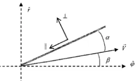
2. 1. Launch Trajectory Model The basic trajectory code model describes a flat plate traveling along a plane around the Earth as shown Figure 1. Radius r and angle
φ represent the vehicle’s position in a polar coordinate system. Using unit vectors
j
ˆ and rˆ associated with this coordinate reference, Vj and Vr described the velocity along those two vectors. The position of the vehicle can then be related to the velocities as follows.r
d dh
r V V
dt j dt
j= =
(1)
Note that h represents the altitude [5]. The velocity vector is at an angle β with
j
ˆ and can be represented as: Vj=Vcos , b V Vr= sinbThe acting forces on the vehicle are as shown on the right diagram of Figure 1. The vehicle’s one weight (Wr) and centrifugal force (FC) are directed along with the rˆ vector. The lift force (Lr) is shown perpendicular and the drag force (Dr) parallel to velocityVr. The thrust vector (Tr) is at anglefTwith velocity Vr.So, the equations of motion of the vehicle become:
2
cos( ) - cos - sin
sin( ) cos - sin T
r T dV
M T D L
dt
V dV
M T L D M Mg
dt r
j
j
f b b b
f b b b
ì
= +
ïï í
ï = + + +
-ïî
(2)
Within the position coordinate system, another coordinate system must be defined. Consider a flat plate at angle of attack α. Unit vectors ॥ and ^ are parallel and perpendicular to the plate respectively as shown in the Figure 2.
Along these unit vectors, forces F॥ and F^ are related to lift and drag forces as follows [6]:
cos sin
sin cos
L F F
D F F
a a
a a
^
^
=
-ì
í = +
î
(3)
Note that the drag force acts in the opposite direction from the velocity.
Substituting Equation (3) into (2), the equations of motion are represented by:
2
cos( ) sin( )
cos( )
sin( ) cos( ) sin( )
+M T
r
T
dV
M T F
dt F dV
M T F F
dt V
Mg r
j
j
f b a b
a b
f b a b a b
^
^
ì = + - +
ï ï
- +
ï ï
í = + + + - +
ï ï
ï
-ïî
(4)
By assuming certain initial conditions at time t = 0, the next velocity components and therefore angle β can be calculated for the next time step using the Equation (4). The following position of the vehicle is recalculated using Equation (1). The altitude during one time step helps compute the air density and aerodynamic forces acting on the vehicle for the following step.
Figure 1. Representation of forces acting on vehicle
Though the thrust angle is initially assumed, there are 3 thrust angles cases that must be considered. First case being that ΦT = 0 and T
r
is always along Vr.The second scenario is where ΦT = α and T
r
is along the chord length. The final case is where ΦT = -β and T
r
is always along
j
ˆ. Since the aerodynamic forces are proportional to the vehicle’s surface area (A), and dynamic pressure (ρV2), we divide both sides of Equation (4) by the vehicle mass to get:2
cos( ) sin( ) cos( )
sin( ) cos( ) sin( )
T r
T
dV T g F F
dt W M M
F
dV T g F
dt W M M
V g r
j
j
f b a b a b
f b a b a b
^
^
ì = + - + - +
ï ï
ï = + + + - +
í ï ï + -ï î (5)
2. 2. Trajectory Model in Near Space Near space is considered to lie between 20-100 km in altitude. It’s a range of very low density. As this altitude is part of the trajectory presented in this research, the forces acting on the vehicle traveling across that altitude also need to be presented [7, 8].
Consider the following scenario where a flux of incident particles reflects off a surface at an angle qi
from the normal. The thermal spreading of these particles can be considered negligible, and angle α is the angle of attack from the surface. The unit area dA on the wall onto which the particles hit project an area
cos i
dA q , as shown in Figure 3 [9]. The flux of particles through this area can be represented as follows [10]:
. . cos i
dF =n u dA q
(6)
For the case of specular reflection (Figure 4), the particle bounces perfectly from the surface at the same angle it arrived at while fully conserving its energy [9]. The momentum and energy transferred to the surface is respectively [10]:
2 cos
0 0
i
dp m u
dp dQ q ^= ì ï = í ï = î (7)
During diffusive reflection, the particles reflect according to Maxwellian distribution. This occurs at material temperature Tm in the half-space of 0< <q p/ 2. The momentum absorbed can be represented by [9]:
( cos )
sin i i
dp m u
dp mu q u q ^= + ì í = î (8)
where, the mean velocity, u at the material temperature Tm [11]:
0.5 2 m kT m u p æ ö
= çè ÷ø
(9)
By multiplying the particle flux with the momentum equations, the tangential and normal forces projected on
the surface are found and shown in the follow equations [5]. ( ) 2 2 2 2 cos 0 cos cos cos sin i i i i i
dF u dA
Specular dF
dF udA u
Diffuse
dF u dA
r q
r q q u
r q q
^ ^ ì = ï í = ïî = + ìï í = ïî (10)
Translating them on to the Cartesian coordinate system, the Equation (10) becomes:
sin cos
cos sin x
y
dF dF dF
dF dF dF
a a a a ^ ^ = - -ìï
í =
-ïî
(11)
The relationship between the unit vectors‖and ^, and the x-y-coordinate system is shown in Figure 2. The forces per unit area are then shown in the follow equations. 2 3 2 2 2 2 2 sin
2 sin cos
sin . sin
. sin cos x y x y df u Specular df u
df u u
Diffuse
df u
r a
r a a
r a u r a
u r a a
ì =
-ï
í =
ïî
ì = -
-ï
í =
ïî
(12)
The coefficient of accommodation paccrepresents the
likelihood the particles will behave more according to a perfect diffuse model than a perfect reflective model. The pacc value of unity would be considered a perfect
diffusive reflection. For simplicity, we assumed this probability to be a constant, though it usually depends on surface conditions, particle energy, incident angle, and other factors [12]. For our case, paccwas assumed to
be 0.1 due to the high temperatures the plate was expected to experience, as well as the cleanliness and smoothness of the plate’s surface assumed [10].
Each particle transfers energy onto the wall in the amount of u2 /2. Meanwhile, the energy lost by the wall when reflecting a particle is the average energy are shown by equation in article [13]. Finally, the wall was assumed to behave like a black body. The resulting equations for the forces and energy transferred per unit area are:
Figure 3. Reflection of incident particles on surface
2 3 2
2 2
2
4
2(1 )sin sin sin .
2(1 )sin cos sin cos .
3
sin . . .sin
2 4
x acc acc acc
y acc acc
m
acc m
df u P P P
u
df u P P
u kT
u
dq u u P T
m
u
r a a a
u
r a a a a
r a r a s
ì = - é - + + ù
ï êë úû
ï
ï é ù
= - +
í ê ú
ë û
ï
ï æ ö
= -
-ï ç ÷
è ø î
(13)
By including thrust, gravity, and centrifugal force that contributed to vehicle’s dynamics, the equations become [10]:
2 3
2
2
2 2
2(1 ) sin sin
sin .
R
2(1 )sin cos sin cos .
x acc acc
acc
y E
acc acc
du
M T A u P P
dt
P u
d u
M T M Mg
dt h
A u P P
u
r a a
u a
n
u
r a a a a
ì = - é - + +
ë ï ï ù ï ú ï û ï í
ï = + - +
ï +
ï
é ù
ï - +
ê ú
ï ë û
î
(14)
The forces can be normalized by the weight, and using an average area mass density (rm) for the vehicle:
2 3
2
2
2 2
2(1 ) sin
sin sin .
R
2(1 )sin cos sin cos . a x acc m acc acc y E a acc acc m T
du g u P
dt W P P u T d u g g
dt W h
u P P
u r a r u a a n r u
a a a a
r
ì = - é - +
ë ï
ï
ï + ù
ï úû
ï í
ï = + - +
ï +
ï
é ù
ï - +
ê ú
ï ë û
î
(15)
Recall that, W=Mg, ra( )h =r0exp(-h h/ )0 ,dh dt/ =u. In addition to the previous equations, the code calculates the Mach number at every point of the trajectory. The following equation was used to find the speed of sound [14]:
/
a= gP r
(16)
where, we used the adiabatic index, γ = 1.4. p represents pressure, and ρ is the density of air.
3. METHODOLOGY
The launch conditions needed to be simulated in varying high altitude environments. This was achieved using the MATLAB software that is now so commonly used in the aerospace and many other industries. The code developed is based on the previously mentioned model that calculates the forces affecting a flat plate as it gains altitude. It takes into consideration air density changes with altitude, angles of attack (α), payload, initial altitudes of launch (h0), and orbital altitude (hF). The
equations used in this code also take into consideration spectral and diffusive reflection for near space
conditions. By adding a few computation boundaries such as achieving desired orbital velocity and altitude, is completed simulation process.
Two modes serve as the initial launch locations, 20 and 40 km with under of 10 AOA (angle of attack) for SAFIR-2 launch vehicle mission. The consideration and initial condition for different modes are shown in Tables 1 and 2. These are altitudes through which current high altitude balloon-based launch system are able to achieve. Because the code supplies information on altitude, distance, density, velocity, forces and Mach numbers at every point of the launch trajectory, a parametric study was possible between all the variables. The parametric modes performed included trade studies between the different variables, pitch angle (θ) and drag coefficients (Cx), altitude (H), and vehicle velocities in
the x-y-direction at varying angles of attack, pressure (P), thrust vector (Pt) and density (R0), as to analyze
which scenario resulted in the best launch. The parametric modes also helped to determine whether the code was giving valid results.
TABLE 1. Simulation Initial Conditions for 20 km
Mode No. Payload (kg) hF
(km)
Altitude (h0), km
Angle of attack (α), deg SAFIR-2 27 240 0 0
(1) 27 300 20 10
(2) 180 240 20 10
TABLE 2. Simulation Initial Conditions for 40 km
Mode No. Payload (kg) hF
(km)
Altitude (h0), km
Angle of attack (α), deg SAFIR-2 27 240 0 0
(3) 27 385 40 10
(4) 330 240 40 10
4. SIMULATION RESULTS AND DISCUSSION
The following texts show the results achieved with the developed code. Table 3 includes the scenarios considered under SAFIR-2 mission specifications. Simulation results are derived for each set of defined modes with respect to performance parameters.
Therefore, we can increase payload to 180 kg with launching from 20 km, 10 AOA and orbital altitude 240 km (Table 1). We can increase orbital altitude to 300 km with launching from 20 km and 10 AOA with supposed payload 27 kg.
km with launching from 40 km and 10 AOA with supposed payload 27 kg.
Now, by comparative simulation, results in 20 and 40 km altitude are shown in following Figures 5-11.
0 50 100 150 200 250 300 0
0.5 1 1.5 2 2.5 3 3.5
4x 10 5
Flight time(sec)
A
lti
tude
(
m
)
SAFIR-2 Mode(1) Mode(2) Mode(3) Mode(4)
Figure 5. Launch vehicle altitude vs. flight time
0 50 100 150 200 250 300 0
1000 2000 3000 4000 5000 6000 7000 8000
Flight time(sec)
V
e
lo
si
ty
(
m
/s
e
c)
SAFIR-2 Mode(1) Mode(2) Mode(3) Mode(4)
Figure 6. Launch vehicle velocity vs. flight time
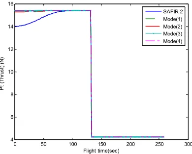
0 50 100 150 200 250 300 4
6 8 10 12 14 16
Flight time(sec)
P
t
(T
hr
us
t)
(
N
)
SAFIR-2 Mode(1) Mode(2) Mode(3) Mode(4)
Figure 7. Launch vehicle thrust vector vs. flight time
0 50 100 150 200 250 300 0
0.1 0.2 0.3 0.4 0.5 0.6 0.7
Flight time(sec)
C
x
(D
rag
C
oe
ff
ic
ie
nt
)
SAFIR-2 Mode(1) Mode(2) Mode(3) Mode(4)
Figure 8. Launch vehicle drag coefficient (CX) vs. time
0 50 100 150 200 250 300 -10
0 10 20 30 40 50 60 70 80 90
Flight time(sec)
q
(
de
g)
SAFIR-2 Mode(1) Mode(2) Mode(3) Mode(4)
Figure 9. Launch vehicle Pitch angle (θ) vs. flight time
TABLE 3. SAFIR-2 Launch Vehicle Specification
stage II stage I
Parameter
Dimensions
3.2 17.20
Length (m)
1.25 1.25
Diameter (m)
Mass
4,000 20,000
Propellant Mass (kg)
4,706 2,1978
Gross Mass (kg)
0.85 0.91
Propellant Mass Fraction
Propulsion
83.4 361.2
Average Thrust (KN) Vacuum
298 280
ISP (sec)- Vacuum
Mission
Launch Site: Semnan, Iran (35.57 deg. N Latitude)
INCL(deg) Attitude (km)
Payload (kg)
55.71 LEO 240
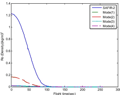
0 50 100 150 200 250 300 0
0.2 0.4 0.6 0.8 1 1.2 1.4
Flight time(sec)
R
o
(D
en
si
ty
)(
kg
/m
3
)
SAFIR-2 Mode(1) Mode(2) Mode(3) Mode(4)
Figure 10. Launch vehicle density (R0) vs. flight time
-1 0 1 2 3 4 5 6 7
x 105 0
0.5 1 1.5 2 2.5 3 3.5
4x 10 5
Range (m)
A
lti
tu
de
(
m
)
SAFIR-2 Mode(1) Mode(2) Mode(3) Mode(4)
Figure 11. Launch vehicle altitude (Y) vs. range (X)
TABLE 4. Developed performance percent of SAFIR-2 launch vehicle mission
In
cre
as
ed
or
bit
al
alt
itud
e
perce
nt
(%)
In
cre
as
ed
pay
loa
d
perce
nt
(%)
h
f
(k
m)
P
ay
load
(k
g)
(
α
) d
eg
h
0
(k
m)
M
ode
--- ---
240 27
0 0
SAFIR-2
--- 566
240 180 10 20
(1)
25 ---
300 27
10 20
(2)
--- 1122
240 330 10 40
(3)
60 ---
385 27
10 40
(4)
Figure 5 shows that with an increase in initial altitude, mass of payload or orbital altitude can be increased considerably under same flight time. The major advantage of this technique is shown in Figure 8- 10. Because of using the standard atmospheric model and specular and diffuse reflection in basic equation of simulation code, drag coefficient and air density are
improved significantly. So, results indicate with a same orbital altitude can increase mass of payload significantly. Furthermore, with a same mass of payload, orbital altitude can be increased in same period of flight time. The major achievement in the innovation and space launch systems is considered.
The developed results for SAFIR-2 mission are shown in Table 4. This table shows the difference between initial height of launch and to surface height. The benefits of using this launch technique for initial altitude is more which makes us appear.
5. CONCLUSION
When comparing all four modes, the first distinct difference was the wider range of angles of attack that the plate could be flown at when launching from the higher altitude of h0 =40 km.
In general, all the flight trajectories remained smoothest at higher T/W ratio. It was also observed that at α =10° results were not favorable at low T/W ratios but improved with larger thrust values. When comparing only the simulation results within one initial altitude, the higher the T/W ratio, the earlier of the supposed orbital alttitude was achieved.
Therfore, the obtained simulation results for each of four modes indicated that for h0 =40 km, increased
percent of payload and orbital alttitde is more desirable. Thus, this technique can be suitable in development and improvement of the next generation launch system missions.
6. REFERENCES
1. Parker, R., "Aircraft and Space Shuttle Accident Rates", Future Pundit , (2008)
2. Nigro, N., Yang, J., Elkouh, A. and Hinton, D., "Generalized math model for simulation of high-altitude balloon systems",
Journal of Aircraft, Vol. 22, No. 8, (1985), 697-704.
3. Kandis, M., Witkowski, A., Machalick, W. and Klein, E., "Energy Modulators for Recovery of High Altitude Balloon Payloads", AIAA Balloon Systems Conference, (2009). 4. Wanagas, J. D. and Gizinski III, S. J., "Small satellite delivery
using a balloon-based launch system", in AIAA 14th International Communication Satellite Systems Conference and Exhibit. Vol. 1, (1992).
5. Sarigul-Klijn, N., Sarigul-Klijn, M. and Noel, C., "Air-launching earth to orbit: effects of launch conditions and vehicle aerodynamics", Journal of Spacecraft and Rockets, Vol. 42, (2005).
6. Anderson, J. D., JR,"Introduction to Flight", Mc Graw-Hill International Editions, Aerospace Science Series, (1995) 7. Browning, W. M., Olson, D. S. and Keenan, D. E.,
8. Runnels, S. R., Smith, M. S. and Fairbrother, D. A., "High-altitude balloon thermal trajectory analysis database system",
AIAA 3rd Annual Aviation Technology, (2003).
9. Potter, J. L., "Rarefied gas dynamics, Wiley Online Library, (2007).
10. Loeb, L. B., "The kinetic theory of gases", Dover Publications, (2004).
11. Collie, C., "Kinetic theory and entropy", Longman, (1982). 12. Shukla, P. K. and Mamun, A., "Introduction to dusty plasma
physics", Taylor & Francis, Vol. 10, (2001).
13. Anderson, J. D., "Hypersonic and high temperature gas dynamics", AIAA, (2000).
Performance Evaluation of a High-altitude Launch Technique to Orbit Using
Atmospheric Properties
M. R. Taheri a, A. Soleymani a, A. Toloeia , A. R. Vali b
aSpace Engineering, New Technologies Engineering Faculty, Shahid Beheshti University, Tehran, Iran, b Department of Electrical Engineering, Maleke Ashtar University of Technology, Iran
P A P E R I N F O
Paper history: Received 28 April 2012
Received in revised form 23 July 2012 Accepted 18 October 2012
Keywords: High Altitude Launch Trajectory Model Atmospheric Conditions Performance Evaluation Near Space
SAFIR-2 Mission
هﺪﯿﮑﭼ
نﺎﮑﻣافﺪﻫﻪﻟﺎﻘﻣﻦﯾارد ردراﺮﻘﺘﺳاﺖﻬﺟصﺎﺧعﺎﻔﺗراﮏﯾزاﯽﯾﺎﻀﻓﻪﻠﯿﺳوﮏﯾبﺎﺗﺮﭘﮏﯿﻨﮑﺗدﺮﮑﻠﻤﻋﯽﺑﺎﯾزراوﯽﺠﻨﺳ
ﯽﻣﻦﯿﻣزﻪﺑﮏﯾدﺰﻧراﺪﻣ ﺪﺷﺎﺑ
.
هﺪﺷدﺎﻬﻨﺸﯿﭘﻪﻟﺎﻘﻣﻦﯾارد
راﺪـﻣﮏـﯾﻪـﺑدﺎﯾزعﺎﻔﺗراﮏﯾزابﺎﺗﺮﭘزاﯽﺗوﺎﻔﺘﻣعﻮﻧﻪﮐﺖﺳا
ﺎﻔﺗرا دﻮﺷﻞﯿﻠﺤﺗوﯽﺳرﺮﺑﻦﯿﯾﺎﭘع
.
مﺎﺠﻧاتﺎﻌﻟﺎﻄﻣﺎﺑﻖﺑﺎﻄﻣﻪﻠﯿﺳوﻻﺎﺑعﺎﻔﺗرابﺎﺗﺮﭘﻪﯿﻟواﻂﯾاﺮﺷﺪﻨﯾآﺮﻓﻦﯾارد
رد،ﻪـﺘﻓﺮﮔ
عﺎﻔﺗراخﺮﻧ
20
ﺎﺗ
40
ﻒﻠﺘﺨﻣيراﺪﻣعﺎﻔﺗراﺖﺤﺗوﻪﻟﻮﻤﺤﻣنزوﻪﺑﺖﺳاﺮﺗﻞﯿﻓوﺮﭘتاﺮﯿﯿﻐﺗﺐﺴﺣﺮﺑﻪﮐهدﻮﺑيﺮﺘﻣﻮﻠﯿﮐ
ﺖﺳاهﺪﺷﯽﺑﺎﯾزرا
.
ﺮﭘﻂﯾاﺮﺷيﺮﯿﮔراﺮﻗﻞﯿﻟدﻪﺑ
تﻻدﺎـﻌﻣ،ﻦﯿﻣزﺮﻔﺴﻤﺗاذﻮﻔﻧﺮﯿﺛﺎﺗﺖﺤﺗوروﺎﺠﻣيﺎﻀﻓهدوﺪﺤﻣردبﺎﺗ
ﻪﯿﺒﺷﯽﻔﯿﻃويذﻮﻔﻧسﺎﮑﻌﻧالﺪﻣودياﺮﺑيزاوﺮﭘﺖﮐﺮﺣﺮﯿﺴﻣﺮﺑﻢﮐﺎﺣ ﺖﺳاهﺪﯾدﺮﮔﻦﯿﯿﻌﺗويزﺎﺳ
.
ﺮﺛاﺶﻫﺎﮐرﻮﻈﻨﻣﻪﺑ
وﺎﺠﻣيﺎﻀﻓتﺎﺷﺎﺸﺘﻏا ﺮﻣاﺖﯾﺎﻬﻧردﻪﮐهﺪﺷﻪﺘﻓﺮﮔﺮﻈﻧردﺖﺨﺗﻪﺤﻔﺻﮏﯾترﻮﺻﻪﺑﯽﺑﺎﺗﺮﭘلﺪﻣ،ﻪﻠﺌﺴﻣﻞﺣﺪﻧورردر
ﻪﯿﺒﺷﺪﻨﯾآﺮﻓ،ﺮﻈﻧدرﻮﻣﻪﻟﻮﻤﺤﻣياﺮﺑفﺪﻫراﺪﻣﻖﯾرﺰﺗﯽﯾﺎﻬﺘﻧاﻂﯾاﺮﺷندوﺰﻓاﺎﺑ ﯽـﻣﻞﯿﻤﮑﺗيزﺎﺳ
ددﺮـﮔ
. ﺖـﻬﺟﻪـﻣادارد
هراﻮﻫﺎﻣﺖﯾرﻮﻣﺄﻣ،ﻪﻠﺌﺴﻣﺞﯾﺎﺘﻧﯽﺠﻨﺳرﺎﺒﺘﻋا ﺮﯿﻔﺳﺮﺑ
-2
ﻪﯿﺒﺷ هدادويزﺎﺳ ﻫ
ﺖﺳاهﺪﺷﻪﺴﯾﺎﻘﻣﯽﺗﺎﯿﻠﻤﻋزﺎﻓﺎﺑﯽﺟوﺮﺧيﺎ
.