Calculation of Complicated Flows, Using First and Second-Order Schemes (RESEARCH NOTE)

RESEARCH NOTE

CALCULATION OF COMPLICATED FLOWS, USING FIRST AND

SECOND-ORDER SCHEMES

M. Goodarzi and A. R. Azimian

Mechanical Engineering Department, Isfahan University of Technology Isfahan, Iran, [email protected]

(Received: December 17, 2001 – Accepted in Revised Form: August 11, 2003)

Abstract The first-order schemes used for discretisation of the convective terms are straightforward and easy to use, with the drawback of introducing numerical diffusion. Application of the second-order schemes, such as QUICK scheme, is a treatment to reduce the numerical diffusion, but increasing convergence oscillation is unavoidable. The technique used in this study is a compromise between the above-mentioned problem, i.e. reducing the numerical diffusion and increasing the stability of the solution. This double folded task is achieved by introducing a modified second-order hybrid scheme. In addition to that by means of this formulation it is possible to show that the coefficients of the discretised equation at all neighboring points are positive and the value of a coefficient at a pole point is equal to the sum of its neighboring points, which means the two basic conditions defined by Patankar are satisfied. Therefore, this scheme has the benefits of the both first and second order schemes together. Results obtained by this scheme to predict the complicated flow regimes were promising and agreed well with experimental data.

Key Words Second-Order Hybrid Scheme, Stability, Boundedness, Numerical Diffusion, Laminar Flows

ﻩﺪﻴﮑﭼ

ﻩﺪﻴﮑﭼ

ﻩﺪﻴﮑﭼ

ﻩﺪﻴﮑﭼ

ﺎﻬﺷﻭﺭﻦﻳﺍ ﺭﺩﺎﻣﺍ ؛ﺖﺳﺍ ﻩﺩﺎﺳﻲﻳﺎﺠﺑﺎﺟﯼﺎﻫ ﻪﻠﻤﺟﻥﺩﺮﮐﻪﺘﺴﺴﮔ ﺭﺩﻝﻭﺍﻪﺒﺗﺮﻣﯼﺎﻬﺷﻭﺭ ﻥﺩﺮﺑﺭﺎﮑﺑ

ﻲﻣﺩﻮﺟﻮﺑ ﯼﺩﺪﻋﻥﮊﻮﻴﻔﻳﺩ ﺪﻳﺁ

. ﺵﻭﺭﺪﻨﻧﺎﻣ ،ﻡﻭﺩﻪﺒﺗﺮﻣ ﯼﺎﻬﺷﻭﺭﯼﺩﺪﻋﻥﮊﻮﻴﻔﻳﺩ ﺶﻫﺎﮐﯼﺍﺮﺑ

QUICK

ﻲﻓﺮﻌﻣ

ﺩﺭﺍﺩﺩﻮﺟﻭﻲﻳﺍﺮﮕﻤﻫﺕﺎﻧﺎﺳﻮﻧﻞﮑﺸﻣﺎﻬﺷﻭﺭﻦﻳﺍﺭﺩﺎﻣﺍ،ﺪﻧﺍﻩﺪﺷ

.

ﺑﻪﻌﻟﺎﻄﻣﻦﻳﺍﺭﺩ

ﻭﯼﺩﺪﻋﻥﮊﻮﻴﻔﻳﺩﺶﻫﺎﮐﯼﺍﺮ

ﺖﺳﺍ ﻩﺪﺷ ﺢﻴﺤﺼﺗﻡﻭﺩ ﺔﺒﺗﺮﻣ ﺪﻳﺮﺒﻴﻫ ﺵﻭﺭﯼﺩﺪﻋ ﻞﺣﯼﺭﺍﺪﻳﺎﭘ ﺶﻳﺍﺰﻓﺍ

. ﻲﺳﺎﺳﺍ ﻁﺮﺷ ﻭﺩ ﺵﻭﺭﻦﻳﺍ ﻪﻠﻴﺳﻮﺑ

ﻩﺮﮔ ﺐﻳﺮﺿ ﯼﺮﺑﺍﺮﺑ ﻭ ﻩﺪﺷ ﻪﺘﺴﺴﮔ ﺕﻻﺩﺎﻌﻣ ﺐﻳﺍﺮﺿ ﻥﺩﻮﺑ ﺖﺒﺜﻣ ﺯﺍ ﺪﻨﺗﺭﺎﺒﻋ ﻪﮐ ﺭﺎﮑﻧﺎﺗﺎﭘ ﻂﺳﻮﺗ ﻩﺪﺷ ﻲﻓﺮﻌﻣ

ﻲﻣﺎﺿﺭﺍﻥﺁﺭﻭﺎﺠﻣﻁﺎﻘﻧﺐﻳﺍﺮﺿﻉﻮﻤﺠﻣﺎﺑﯼﺰﮐﺮﻣ ﺪﻧﻮﺷ

.

ﺍﺮﺑﺎﻨﺑ

ﻝﻭﺍﻪﺒﺗﺮﻣﯼﺎﻬﺷﻭﺭﯼﺎﻳﺍﺰﻣﻩﺪﺷﻲﻓﺮﻌﻣﺵﻭﺭﻦﻳ

ﺩﺭﺍﺩﻢﻫﺎﺑﺍﺭﻡﻭﺩﻭ

. ﻖﺑﺎﻄﺗﻭﺪﻨﺘﺴﻫﺐﻟﺎﺟﺵﻭﺭﻦﻳﺍﻂﺳﻮﺗﻩﺪﻣﺁﺖﺳﺪﺑﺞﻳﺎﺘﻧ،ﻩﺪﻴﭽﻴﭘﯼﺎﻬﻧﺎﻳﺮﺟﯽﻨﻴﺑﺶﻴﭘﺭﺩ

ﻲﻣﻥﺎﺸﻧﻲﺑﺮﺠﺗﺞﻳﺎﺘﻧﺎﺑﻲﺑﻮﺧﺭﺎﻴﺴﺑ ﺪﻨﻫﺩ

.

1. INTRODUCTION

The convective terms with nonlinear behavior have a basic role in the solution of the Navier-Stokes equations, and are very important. Convergence, stability, and accuracy of the results are strongly dependent on the way that these terms are discretised. Therefore, appropriate discretisation schemes are required to treat these terms, and several schemes have been proposed for these terms, with their merits and deficiencies. Basically first-order schemes such as hybrid central / upwind (HYBRID), and the power-law schemes [1], cause

numerical diffusion. This problem becomes more sever when the flow direction is skewed relative to the grid lines. As an example, it is possible to mention a three-dimensional flow with secondary flows, where the numerical diffusion may become greater than the physical diffusion [2]. Nevertheless these schemes are unconditionally bounded and highly stable.

has been reduced. However, these schemes suffer from the boundedness problem and have oscillations in the region of steep gradients. Stability and accuracy of the first and higher order schemes is an important issue, which was examined by Leonard [3].

To develop oscillation-free high-order schemes, two important concepts (i.e. monotonocity [6], and bounded total variation [7]) have been introduced. For monotone or total variation diminishing (TVD) schemes, several methods have been developed. The Flux-Corrected Transport (FCT) algorithm, introduced by Zalesak [8] is one among the many others.

In this study a modified version of the Li and Rudman scheme [9], in which a Peclet number dependent parameter for the second-order hybrid scheme was introduced, is used. This scheme is capable of predicting complicated flow regimes with reduced numerical diffusion and minor stability problems.

2. GENERALIZED FORMULATION FOR FOUR-POINT SCHEMES

The governing equations for a laminar incompressible

steady flow are continuity, and momentum equations. All of these equations could be represented by a general conservative form of the transport equation. The conservative form of the transport equations for the dependent variable,

φ

, in a generalized coordinate system

x

j[10] can be written as

φ

φ

=

∂

φ

∂

Γ

−

φ

ρ

∂

∂

JS

)

x

D

J

U

(

x

m

j m j

j (1)

where

U

_j is the contravariant velocity component, j

m

D

is the geometric coefficient introduced by transformation from the Cartesian coordinates

y

j

to the general coordinate system,

ρ

is the fluid density,

Γ

_φ is the diffusion coefficient,

S

_φ is the source term for dependent variable

φ

, and J is the Jacobian. For continuity equation

φ

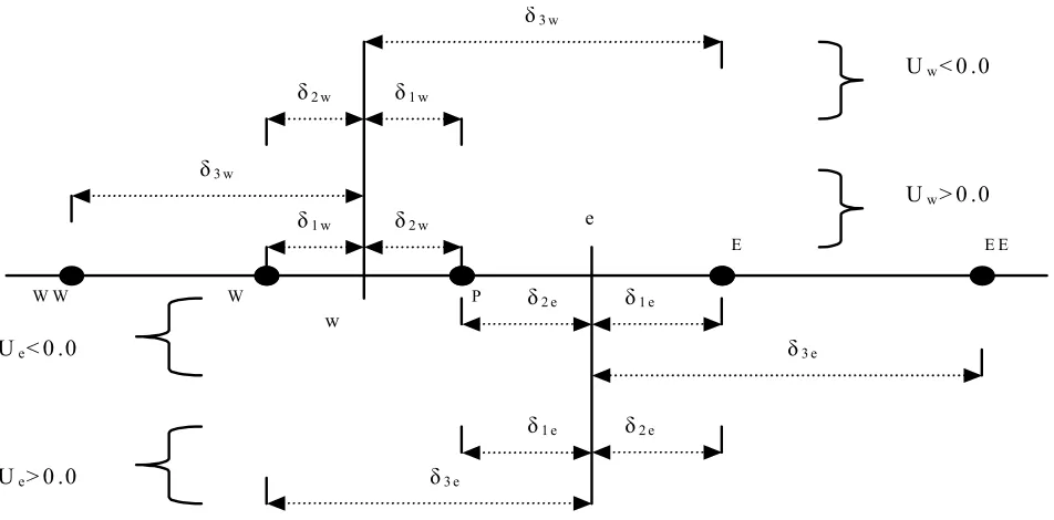
is equal to 1 and for momentum equations it is equal to u, v, and w, respectively.

Without loosing generality, it is possible to use the Cartesian form of the transport equations. In the following the derivation of the equations have been explained, and the notation of the Patankar δ3 w

P W

E E E

W W

e

w δ1 w

δ1 w

δ2 w

δ2 w

δ1 e

δ1 e

δ2 e

δ2 e

δ3 e

δ3 e

δ3 w

Uw> 0 .0

Uw< 0 .0

Ue> 0 .0

Ue< 0 .0

[1] has been employed. In a finite control volume approach, integration of the convective terms in equation (1) for a two dimensional case will result:

∫∫

ρ

φ

=

φ

−

φ

+

φ

−

φ

∂

∂

s s n n w w e e i i

F

F

F

F

dV

)

u

(

x

(2) where

F

_i

=

ρ

u

_i

A

_i, is the mass flux from ith face

of the control volume with area

A

_i, and indices e, w, n, and s denote the east, west, north and south faces respectively. In Figure 1 the notation used to define the nodes and grid parameters in x-direction are shown. Nondimensional grid parameters could be written as follows

w 1 w 3 w 3 w 2 w 2 w 1 w 3 w 2 w 1 w 1

δ

−

δ

δ

+

δ

=

β

δ

−

δ

δ

+

δ

=

β

w 2 w 1 w 2 w 2 w 2 w 1 w 1 w 1

δ

+

δ

δ

=

α

δ

+

δ

δ

=

α

(3)

As an example it is possible to write the generalized form of the four-point scheme for an interpolated value of

φ

_w on the west face

0

.

0

u

_w

>

) (

q_{w P 2w W 1w WW}

P w 1 W w 2

w =α φ +α φ − φ −β φ +β φ

φ

0

.

0

u

_w

<

) (

qw W 2w P 1w E

P w 2 W w 1

w =α φ +α φ − φ −β φ +β φ

φ

(4) The value of the parameter

q

_w used in Equation 4,

depends on the scheme being used. For example, in the central difference scheme (CD)

q

_w

=

0

.

0

, in the QUICK scheme

q

_w

=

α

_1w

δ

_2w

/(

δ

_2w

+

δ

_3w

)

and in the second-order upwind scheme (SOU) w

1 w

q

=

α

.

By linearizing the source term in Equation 1 as C

P

P

S

S

φ

+

, and integrating diffusion terms in transport equation, after some manipulations the discretised form of the transport equation based on

the nodal point values would be:

S

a

a

a

a

a

_P

φ

_P

=

_E

φ

_E

+

_W

φ

_W

+

_N

φ

_N

+

_S

φ

_S

+

(5) Based on the values of the parameter

q

, these coefficients are either negative or positive. As Patankar recommended, all of the coefficients of nodal points must be positive values. To solve this problem a minimization method, in which

q

is defined based on the Peclet number and the grid parameters, are used as follows

        − α = ) P 1 ( , 0 . 0 max q w e w 1

w (6)

Using the above-mentioned definition, the scheme that is referred to as a Second-order Hybrid scheme (SHYBRID), uses the advantages of the first and second order schemes together. Li and Rudman [9] studied the details of analysis of the total variation diminishing (TVD) and boundedness for this formulation.

Another Patankar recommendation states that, in the absence of source term in Equation 1 the sum of the values of the coefficients at the neighboring points must be equal to the value of the coefficient at the pole point. So it is decided to derive the coefficients in a modified version of the Li and Rudman [9], which originally had not this characteristic, as follows.

The upwind mass flow rates over each face of the control volume are introduced as follows:

2

F

F

F

_w−

=

w

−

w

2

F

F

F

_w+

=

w

+

w ₍₇₎

From Equation 3 the following relation between the geometric parameters can be derived:

1

1

w 1 w 2 w 2 w 1

=

β

−

β

=

α

+

α

(9)

Inserting Equation 9 in Equation 8, and making suitable factorization, the right hand side of Equation 8 can be written as follows:

) F F F F ( F q ) ( F q ) ( ) F q F q F F q F )( ( ) F q F q F F q F )( ( w w e e P w w 1 w WW W e e 1 e EE E e e 1 e w w w w 2 w w w w 1 W P w w 1 w e e e e 2 e e e e 1 P E − + − + + − + + + − − − − − + + − − + φ + β φ − φ − β φ − φ + β + + α + − α φ − φ + β + + α + − α φ − φ (10) Similar expressions for

F

_n

φ

_n

−

F

_s

φ

_s could be

written. Therefore, by adding the diffusion terms, and the linearized form of the source term to the convective terms, the coefficients derived by this scheme could be written as follows:

C s s 1 s S SS w w 1 w W WW e e 1 e E EE e e 1 e E EE s n w e P S W N E P s n n 1 n s s s 2 s s s 1 S w e e 1 e w w w 2 w w w 1 W n s s 1 s n n n 2 n n n 1 N e w w 1 w e e e 2 e e e 1 E S F q ) ( F q ) ( F q ) ( F q ) ( S ) F F F F ( S a a a a a D F q F ) q ( F ) q ( a D F q F ) q ( F ) q ( a D F q F ) q ( F ) q ( a D F q F ) q ( F ) q ( a + β φ − φ − β φ − φ − β φ − φ + β φ − φ = − + − + − + + + = + β + + α + − α + = + β + + α + − α + = + β − + α − − α − = + β − + α − − α − = + + − − + + − + + − − − + − − + (11) in which i 2 i 1 i i i

A

D

δ

+

δ

Γ

=

i

=

w

,

e

,

s

,

n

(12)

Considering the continuity equation, the last term in the right hand side of the relation for

a

_P is

equal to zero. Now, by assuming

S

=

₀

.

₀

φ in Equation 1, it can be easily shown that:

∑

=

=

4 1 nb nb P

a

a

(13)

With this formulation the coefficients of the all-neighboring points are positive and the value of a coefficient at a pole point is equal to the sum of its neighboring points. With this manipulation two basic conditions defined by Patankar [1] for numerical algorithms are satisfied. These conditions are as follows: 1) All coefficients must be positive, and 2) the pole coefficient must be equal to the sum of its neighboring points. Also this new formulation can be easily programmed and used in CFD (Computational Fluid Dynamics) codes, which considerably simplifies the formulation of the coefficients for all internal and boundary nodes.

3. APPLICATION OF THE QUICK, FIRST, AND SECOND-ORDER HYBRID SCHEMES

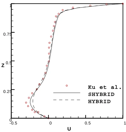
of the cavity are shown in Figure 3. Also the analytical results of the Ku et al [12] are combined in the same figure. As it is shown in this figure, the velocity profile predicted by the second-order hybrid scheme is better than the first-order result, especially in the recirculating regions.

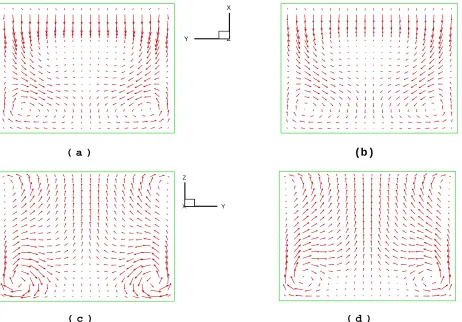
Figure 4 shows the predicted secondary flows in the two center planes of the cavity. This figure shows that, the vortices predicted by the

second-order hybrid scheme are more visible than that of the first-order case. The diffusive behavior of the first-order scheme causes vortices in the cavity to combine together and form a single large vortex. Therefore these vortices are not as strong as those obtained by the second-order hybrid solution.

Laminar Flow in a Square Duct with a 90

°

Bend

In Figure 5 the geometry of a square duct with a 90° bend is shown. The flow in this geometry has a three-dimensional pattern with strong secondary flows, which are caused by centrifugal forces and the pressure gradients across the bend. Humphry et al. [13] experimentally studied this problem and their test data was used for comparison. The numerical solution was based on their experimental Reynolds number of 790, which was calculated based on the hydraulic diameter of the duct and the bulk velocity. Due to the symmetry of the duct, only one half of the domain was solved, and a nonuniform grid system with 47x32x17 mesh points was selected.

To obtain the flow pattern inside the bend, three different numerical schemes were used. These schemes are the first-order hybrid scheme, the order hybrid scheme, and also the second-order QUICK scheme. The parameter q, which was introduced in Equation 4, determines that the second-order scheme is either QUICK or SHYBRID. It is worth mentioning that, since the modified second-order hybrid scheme has less stability problem in numerical procedure, we could choose a greater under-relaxation coefficient than that for QUICK scheme to solve the problem. In Figure 6 the predicted velocity profiles obtained by the three different numerical schemes at the exit plane of the bend are compared with the experimental results. These comparisons are shown at two values of z/b (i.e. z/b = 0.5 and z/b = 1.0), which z is the distance from the rigid boundary and b is the one half of the width of the duct. As it is shown in this figure, the velocity profiles predicted by the first-order hybrid scheme show a more flat pattern at the exit plane of the 90° bend, because in first-order hybrid scheme the numerical diffusion is greater than the second-order ones.

To present the numerical results through the entire bend, ten streamwise cross-sections inside the bend at intervals of 10° were selected. The first cross-section was at the zero angle (i.e. at the

U

x

y

z

Figure 2. Geometry of square cavity.

-0.5 0 0.5 1

U

0 0.25 0.5 0.75 1

Z

Ku et al. SHY BRID HYB RID

beginning of the bend ), and the last cross-section was at the 90° angle (i.e. at the exit plane of the bend ). In Figure 7 the secondary flow formation in the 90° bend predicted by HYBRID scheme is

shown, while in Figures 8 and 9 the same results obtained for SHYBRID and QUICK, are presented respectively. A comparison of these figures shows that the results obtained by the second-order schemes (i.e. SHYBRID and QUICK) are much better than the results obtained by a first-order scheme (i.e. HYBRID). The numerical diffusion introduced by the first-order scheme is the source of this weakness. Close examination of Figures 8 and 9 shows that the mechanism of the vortex formation in both SHYBRID and QUICK schemes are similar. However, the positions of the main vortices are not exactly the same and the difference is much clear at angular position of 70°. Also, there is no need to mention that the accuracy of the results obtained by the new scheme is much better than the other schemes (i.e. HYBRID and QUICK). Another important point to be mentioned in these figures (i.e. from 7 to 9) is the movement of the vortices away from the axis of the symmetry toward the solid wall. This in fact is due to the

( b )

X

Y Z

( a )

X Y

Z

( c ) ( d )

Figure 4. Secondary flows in two centerplane, (a) and (c) SHYBRID, (b) and (d) HYBRID.

Ro=112 mm

R

i₌₇

2 mm

z

b

y

x

1.2 m

1.8 m

0 0.2 0.4 0.6 0.8 1 (R-Ri)/(Ro-Ri)

0 0.5 1 1.5 2

Exp.

Hybrid

Quick

SHybrid

z/b = 1.0

0 0.2 0.4 0.6 0.8 1

(R-Ri)/(Ro-Ri) 0

0.5 1 1.5 2

U

teta/

Us

Exp.

Hybrid

Quick

SHybrid

z/b = 0.5

Figure 6. Predicted Uθ-velocity profile at 90° plane.

centrifugal forces in the bend, which pushes the vortices toward the wall.

4. CONCLUSION

A modified second-order hybrid formulation for discretisation of convective terms in the Navier-Stokes equations was proposed. In this scheme in addition to improve stability condition and reduced numerical diffusion, which is the characteristic of the most of the second-order schemes, two well known criteria set by Patankar [1] are satisfied (i.e. all coefficients are positive and the sum of the values of the coefficients at the neighboring points are equal to the value of the coefficient at the pole point). With these two conditions satisfied, the programming would be much easier, faster, and as

mentioned earlier the stability would be improved further. This is a very useful achievement and could be implemented in the most CFD codes of this nature. In fact, since this scheme is almost free from convergence oscillation problem, it could be considered as a proper alternative for second-order schemes that have boundedness problem.

5. NOMENCLATURE

Ai areas of the finite volume faces (i = w,e,s,n denotes the various directions)

i

a

coefficients in the finite difference equations (i=W,E,S,N,P,WW,EE,SS,NN)

i

D

diffusion coefficients in the finite difference equations (i = w,e,s,n)

j m

D

geometric parameter computed from coordinate transformation

i

F

mass fluxes from the finite volume faces (i = w,e,s,n)

J Jacobian of the coordinate transformation Pe Peclet number

i

q

parameter for the generalized four- point schemes (i = w,e,s,n)

Sф source term of the dependent variable in

the transport equation

Uj contravariant velocity components (i = w,e,s,n)

uk Cartesian velocity components xj _{general coordinate axis} yj Cartesian coordinate axis

ij

α

grid parameters ij

β

grid parameters

φ

Γ

diffusion coefficient for dependent variable ij

δ

grid distances

ρ

density of the fluid

i

φ

dependent variable (i=W,E,S,N,P, WW, EE, SS, NN, w, e, s, n)

6. REFERENCES

1. Patankar, S. V., “Numerical Heat Transfer and Fluid Flow”, Hemisphere, Washington, DC, (1980).

2. de Vahl Davis, G. and Mallinson, G. D., “An Evaluation of Upwind and Central Difference Approximations by a Study of Recirculating Flow”, Comp. Fluids, Vol. 4,

(1976), 29-43.

3. Leonard, B. P., “A Stable and Accurate Convective Modeling Procedure Based on Quadratic Interpolation”,

Comp. Meth. Appl. Mech. Eng., Vol. 19, (1979), 59-98.

4. Shyy, W., “A Study of Finite Difference Approximation to Steady State Convection Dominated Flows”, J. Comp. Phys., Vol. 57, (1985), 415-438.

5. Raithby, G. D., “Skew Upstream Differencing Schemes for Problem Involving Fluid Flow”, Comp. Meth. Appl. Mech. Eng., Vol. 9, (1976), 153-164.

6. Hirsch, C., “Numerical Computation of Internal and External Flows”, Vol. 2, Chap. 21, John Wiley, New York, (1988).

7. Harten, A., “High Resolution Schemes for Hyperbolic Conservation Laws”, J. Comp. Phys., Vol. 49, (1983), 357-393.

8. Zalesak, S. T., “Fully Multidimensional Flux- Corrected Transport Algorithms for Fluids”, J. Comp. Phys., Vol.

31, (1979), 335-362.

9. Li, Y. and Rudman, M., “Assessment of Higher- Order Upwind Schemes Incorporating FCT for Convection-

Dominated Problems”, Numerical Heat Transfer, Part B,

27, (1995), 1-12.

10. Choi, S. K., Nam, H. Y. and Cho, M., “Evaluation of a Higher- Order Bounded Convection Scheme: Three- Dimensional Numerical Experiments”, Numerical Heat Transfer, Part B, 28, (1995), 23-38.

11. Rhie, C. M. and Chow, W. L., “Numerical Study of the Turbulent Flow Past an Airfoil with Trailing Edge Separation”, AIAA J., Vol. 21, (1983), 1525-1532.

12. Ku, H. C., Hirsch, R. S. and Taylor, T. D., “A Pseudo-spectral Method for solution of the Three- Dimensional Incompressible Navier-Stokes Equations”, J. Comp. Phys., Vol. 70, (1987), 439-462.

13. Humphrey, J. A. C., Taylor, A. M. K. and Whitelaw, J. H.,