Fault Detection of Bearings Using a Rule-based Classifier Ensemble and Genetic Algorithm

(1)

Please cite this article as: M. Heidari, Fault Detection of Bearings Using a Rule-based Classifier Ensemble and Genetic Algorithm, International Journal of Engineering (IJE), TRANSACTIONS A: Basics Vol. 30, No. 4, (April 2017) 604-609

International Journal of Engineering

J o u r n a l H o m e p a g e : w w w . i j e . i r

Fault Detection of Bearings Using a Rule-based Classifier Ensemble and Genetic

Algorithm

M. Heidari*

Department of Mechanical Engineering, Aligudarz Branch, Islamic Azad University, Aligudarz, Iran

P A P E R I N F O

Paper history: Received 30 October 2016

Received in revised form 04 February 2017 Accepted 26 February 2017

Keywords: Fault Detection Bearing

Classifier Ensemble Genetic Algorithm

A B S T R A C T

This paper proposes a reduct construction method based on discernibility matrix simplification. The method works with genetic algorithm. To identify potential problems and prevent complete failure of bearings, a new method based on rule-based classifier ensemble is presented. Genetic algorithm is used for feature reduction. The generated rules of the reducts are used to build the candidate base classifiers. Then, several base classifiers are selected according to their diversity and the scale of them. Weights of the selected base classifiers are calculated based on a measure of support rate. The classifier ensemble is constructed by the base classifiers. The accuracy reached 98.44% which is 4.5% higher than that of the three base classifiers.

doi: 10.5829/idosi.ije.2017.30.04a.20

1. INTRODUCTION1

Data analysis, dependency analysis, and learning are some of the most important applications of rough set theory. In those applications, it is typically assumed that we have a finite set of objects described by a finite set of attributes. The values of objects on attributes can be conveniently represented by an information table, with rows representing objects and columns representing attributes. Failures of rotary machineries is a vital problem in plants which are expected for a long running of machines. There is an increasing demand for techniques able to utilize the sensor data to diagnose faults of rotary machineries. The faults arising in rotating machines are usually caused by damages and failures in bearings, gears and shafts. There are some variations in vibration signals of bearings when faults happen. Several advantages for machine condition monitoring and fault diagnosis, as reducing maintenance costs, improving productivity and increasing machine availability, were formerly reported. Bearing is one of the most vital components in the industries. The importance and need to the bearing is clear; therefore,

*Corresponding Author’s Email: [email protected] (M. Heidari)

fault diagnosis of bearings is a core research area in the condition monitoring field [1]. Variations of the vibration signal are either small or buried in strong noises, and cannot be detected easily from vibration signals. To solve these problems, the signal processing and feature extraction are performed first. The wavelet transform, empirical mode decomposition (EMD), local mean decomposition (LMD) and their improved method have been widely used to get the components with high signal-noise ratio, based on which features are extracted to describe the symptoms of bearings. Heidari et al. [2] used wavelet transform for fault diagnosis of bearing and gears of a gearbox. Six

dimensionless time-domain features and five

dimensionless frequency-domain features were

(2)

605 M. Heidari / IJE TRANSACTIONS A: Basics Vol. 30, No. 4, (April 2017) 604-609

maintainability for fault diagnosis of two different types of bearings [5]. The fuzzy lattice classifier (FLC) and fuzzy lattice reasoning (FLR) were applied for faults diagnosis of bearing [6]. The rule-based method gave classification results based on the rules in the form of ‘if condition type’. The advantage of this method was that they were much more transparent in decision making process. In this paper, rule-based fault diagnosis by semantic attributes is carried out using an ensemble of classifiers. The motivation behind the use of a classifier ensemble was that ensembles were proved to provide accuracies higher than any of the single base classifiers that constituted them [7]. Furthermore, reliance on different classifiers rendered the reasoning more robust. Yu [8] proposed a new manifold learning algorithm, joint global and local/nonlocal discriminant analysis, which aimed to extract effective intrinsic geometrical information from the given vibration data. Comparisons with other regular methods, principal component analysis, local preserving projection, linear discriminant analysis and local LDA, illustrate the superiority of GLNDA in machinery fault diagnosis. Yijing et al. [9] proposed an adaptive multiple classifier system named AMCS to cope with multi-class imbalanced learning, which makes a distinction among different kinds of

imbalanced data. The AMCS included three

components, which were, feature selection, resampling and ensemble learning. Each component of AMCS was selected discriminatively for different types of imbalanced data. Rathore and kumar [10] presented ensemble methods for the prediction of number of faults in the given software modules. The experimental study was designed and conducted for five open-source software projects with their fifteen releases, collected from the PROMISE data repository. The results were evaluated under two different scenarios, intra-release prediction and inter-releases prediction. The prediction accuracy of ensemble methods was evaluated using absolute error, relative error and measure of completeness performance measures. In addition, a new classifier combination rule based on the consensus approach of different classification algorithms during the ensemble modelling phase has been proposed [11]. The remainder of the paper has been arranged as follows:

Section 2 describes the construction of base classifiers. Overview of classifier ensembleis presented in Section 3. More details of modeling with proposed method and the simulation results are given in Section 4; the paper is concluded with Section 5.

2. CONSTRUCTION of BASE CLASSIFIERS

Feature reduction is used with a method based on the rough set (RS) [12] and genetic algorithm (GA). Rough set theory is one of the mathematical tools that deals

with feature reduction to find a minimal subset. The basic concept is by making an upper and a lower approximation of the data set. The feature reduction is achieved by comparing equivalence relations generated by feature sets considering the dependency degree as an important measure; features are removed and the reduced feature set provides the same dependency degree as the original. The base classifiers utilized the rules generated on the basis of the reducts of features to identify fault of the bearings.

2. 1. Discernibility Matrices Two objects are discernible if their values are different in at least one attribute. Skowron and Rauszer [13] suggested a matrix representation for storing the sets of attributes that discern pairs of objects, called a discernibility matrix. An information table (IT) can be defined as follow:

𝐼𝑇 = (𝑈, 𝐴, 𝑉) (1)

𝐴 = 𝐶 ∪ 𝐷 (2)

𝑈 = {𝑥1, 𝑥2, … , 𝑥𝑚} (3)

𝐶 = {𝑎1, 𝑎2, … , 𝑎𝑛 (4)

𝐷 = {𝑑} (5)

where U is a non-empty finite set of objects, A is a non-empty finite set of attributes and V is a value set of A. An information table represents all available information and knowledge. That is, objects are only perceived, observed, or measured using a finite number of attributes. In Equation (3), 𝑥𝑖 (i=1, 2, …, m) indicates

the ith object. In Equation (4), 𝑎𝑗 (j=1, 2, …, n)

indicates the jth condition attribute. Also parameter d

shows the decision attribute. The discernibility matrices of IT is a 𝑚 × 𝑚 matrices. Each entry 𝑒𝑖,𝑗consists of the

set of attributes that can be used to discern between objects 𝑥𝑖 and 𝑥𝑗 (j=1, 2, …, m) [14],

𝑒𝑖,𝑗= {

{𝑎𝑘∈ 𝐶|𝑎𝑘(𝑥𝑖) ≠ 𝑎𝑘(𝑥𝑗), 𝑑(𝑥𝑖) ≠ 𝑑(𝑥𝑗) ∅, 𝑑(𝑥𝑖) = 𝑑(𝑥𝑗)

𝐸 = {𝑒𝑖,𝑗|𝑒𝑖,𝑗≠ ∅}

(6)

2. 2. Feature Reduction by GA The GA is a heuristic for function optimization, where the minima or maxima of the function cannot be built analytically. A population of potential solutions is refined iteratively by employing a strategy inspired by Darw inistic evolution or natural selection. The GA promotes “survival of the fit test” [15]. It has been used successfully in many fields for optimization problems [16, 17]. In this paper, feature reduction is a process to compute minimal hitting sets [9] of the discernibility matrices. The GA is employed to solve the problem. The fitness function 𝑓1

(3)

𝑓1(𝐵) = (1 − 𝛼). |𝐶|−|𝐵|

|𝐶| + 𝛼. min {𝜀,

|{𝑒∈𝐸|𝑒∩𝐵≠∅}|

|𝐸| } (8)

In Equation (8), symbol ||, α and ε are the length of a set, a weighting between subset lengths and hitting fraction and a minimal value for the hitting fraction, respectively. The subsets B of C are found through the evolutionary search driven by the fitness function and are “good enough” hitting sets, i.e., have a hitting fraction of at least ε, and are collected as reducts in a candidate collection.

3. CONSTRUCTION of CLASSIFIER ENSEMBLE

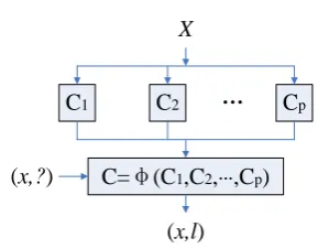
Each reduct in the above candidate set can be used as an independent classifier with its rules generated. Several of them can also be combined together to construct a classifier ensemble. Figure 1 shows the diagram of a classifier ensemble. A set of different base classifiers {𝐶1, 𝐶2, … , 𝐶𝑝} are constructed from a labelled data set

X.

A popular pair wise diversity measure according to the correlation between the performances of the two classifiers (the numbers of patterns correctly/wrongly classified) is adopted. Let i and j be a pair of base classifiers. The correlation between the outputs of i and

j can be measured as:

𝑐𝑜𝑟𝑟𝑖,𝑗= 𝑁

11_𝑁00_−𝑁01_𝑁10

√(𝑁11_+𝑁10_)(𝑁01_+𝑁00_)(𝑁11_+𝑁01_)(𝑁10_+𝑁00₎ (9)

where 𝑁𝑎𝑏_{is the number of test patterns classified}

correctly (a = 1) or incorrectly (a = 0) by the classifier i

and correctly (b = 1) or incorrectly (b = 0) by the classifier j. Classifiers that tend to recognize the same patterns correctly will have positive values of 𝑐𝑜𝑟𝑟𝑖,𝑗,

whereas those which commit errors on different patterns will render 𝑐𝑜𝑟𝑟𝑖,𝑗 negative. A correlation-based

diversity index between classifiers i and j can then be defined based on the correlation coefficient of Equation (9) as:

𝑑𝑖𝑣𝑖,𝑗= 1−𝑐𝑜𝑟𝑟𝑖,𝑗

2 (10)

C1 C2 Cp

C=φ(C1,C2,…,Cp)

… X

(x,?)

(x,l)

Figure 1. Diagram of a classifier ensemble

For a classifier ensemble G consists of more than two classifiers, its diversity index is calculated based on the average of diversity indexes of every pair of classifiers in G as:

𝑑𝑖𝑣(𝐺) =_{|𝐺|(|𝐺|−1)}2 ∑ 𝑑𝑖𝑣𝑖,𝑗 |𝐺|(|𝐺|−1)

2

𝑖,𝑗=1,𝑖<𝑗 (11)

The GA is adopted to select the optimal combination of base classifiers considering the diversity and scale of the ensemble. The fitness function 𝑓2is defined below:

𝑓2(𝐺) = (1 − 𝛽). ( |𝐻|−|𝐺|

|𝐻| ) + 𝛽. 𝑑𝑖𝑣(𝐺) (12)

In Equation (12), H and 𝛽 are the collection of all base classifiers and a weighting between the diversity and scale of the ensemble, respectively. An improved approach based on the static weighted voting (SWV) [18] is developed to integrate the predictions of the base classifiers in this paper. The SWV method involves in assigning a unitary vote to each base classifier 𝐶𝑘, 𝑘 =

1,2, … , 𝑝, and in multiplying that vote by a weight 𝜔𝑘∈ [0,1] proportional to the accuracy of the classifier

measured in terms of the mean recognition rate (MRR), i.e. the fraction of patterns it correctly classifies. In this respect, a third set is required to compute the weights of the base classifiers. However, the 𝜔𝑘 used in the SWV

is a measure of accuracy on the whole despite of a specific class l. Since the classification is implemented with rules, a measure called support rate (SR) is used to replace the MRR. It is defined as:

𝑆𝑅𝑘,𝑙= 𝑁𝑐𝑘,𝑙

𝑁𝑎𝑘,𝑙 (13)

In Equation (13), 𝑁𝑐𝑘,𝑙 and 𝑁𝑎𝑘,𝑙 are the number of

objects which are correctly assigned to class l by kth base classifier and the number of objects which are assigned to class l by kth base classifier, respectively. Each class l of the qth test object receives an ensemble vote given by the sum of all weights assigned to that class:

𝑣_𝑙𝑞= ∑𝑝𝑘=1𝑆𝑅𝑘,𝑙. 𝛿𝑙,𝑘 (14)

Finally, the qth test object is assigned to the class 𝑙𝑞

with the highest ensemble vote:

𝑙𝑞= arg (𝑚𝑎𝑥1≤𝑙≤𝑟(𝑣𝑙 𝑞

)) (15)

where, r is the total number of classes.

4. MODELLING in FAULT DIAGNOSIS with VIBRATION SIGNAL

Vibration signals were obtained from the bearing data center [19]. Bearing of the motor shaft was SKF6203.

(4)

considered. Vibration signal of each condition of bearing was collected by accelerometers, which were attached to the housing of fan end bearings. The sampling frequency was 12000 Hz. Vibration signals were obtained under the speed of 1730, 1750, 1772 and 1797 r/min. The EMD method is used to decompose the 320 signals into IMFs separately. IMF is intrinsic mode function. An IMF is defined as a function that satisfies the following requirements:

1. In the whole data set, the number of extrema and the number of zero-crossings must either be equal or differ at most by one.

2. At any point, the mean value of the envelope defined by the local maxima and the envelope defined by the local minima is zero.

It represents a generally simple oscillatory mode as a counterpart to the simple harmonic function. By definition, an IMF is any function with the same number of extrema and zero crossings, whose envelopes are symmetric with respect to zero. This definition guarantees a well-behaved Hilbert transform of the IMF [20]. Then, the same features used in the literature [3] are extracted on the first IMF for comparison of the two methods. These included six time-domain parameters, i.e. shape factor (SI), impulse factor (IF), crest factor (CF), clearance indicator (CI), skewness (SK), and kurtosis (KI), and five frequency-domain features, i.e. FT, FC, FI, FO and FB. In the other word, FT and FC are fundamental train frequency and combined fault frequency of bearing, respectively.

Also, FI, FO and FB are fault frequencies relationship with inner race fault, outer race fault and ball fault of bearing, respectively. An example of the fault decision (Dec) table (a kind of IT defined in Equation (1)) was given in Table 1, where NC, IRF, ORF, BF indicated the normal condition, inner race fault, outer race fault, and ball fault, respectively.

4. 1. Fault Diagnosis of Bearing Flow chart of the fault diagnosis in bearing is described in Figure 2. In the first step, fault decision table containing 320 objects

is discretized and partitioned into XTRN, XIND and XTST at a ratio of 3:3:2.

Afterward, base classifiers are obtained by performing the GA with its fitness function defined in Equation (8) on the XTRN. Then, base classifiers is selected to construct a classifier ensemble by GA on the XIND. Next, the XIND is used to determine the weights of each base classifier. Finally, the performance of the classifier ensembleis evaluated by the XTST.

4. 2. Results Firstly, discretization was done. The mean of each feature was calculated, and the values in the vector which were less than the mean were designated to zero, otherwise were assigned to one. Zero and one indicated the low level and high level of the index, respectively. Perform the GA with its fitness function defined in Equation (8) on the XTRN, where α=0.33, ε=0.85. The initial population of GA was 70, probability of one-point crossover was 0.3 and probability of mutation was 0.05. 13 reducts were output. Their accuracy of fault classification on XTRN ranged from 78 to 100%. Scale of them ranged from 4 to 10. The large-scale reducts had higher accuracy on the training set, their generalization ability was usually not very good. At this point of view, reducts containing 5 features were put into the candidate collection. They are listed in Table 2.

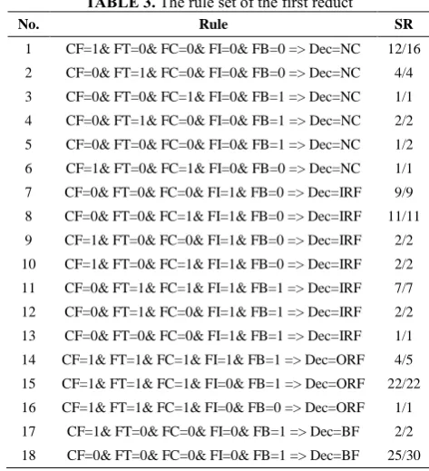
Each reduct had a corresponding rule set. For example, 18 rules were generated based on the first reduct in Table 2. They were given in Table 3.

Classify objects in XIND using the reduct in the candidate collection and its generated rule set. Perform the GA with its fitness function defined in Equation (12) with 𝛽 =0.65. The searching result showed that {{CF,FT,FC,FI,FB},{SK,FT,FC,FI,FB},{CF,SK,FT,FC, FI}} was a good enough choice balancing the diversity against the scale. The weights of 𝑆𝑅𝑘,𝑙 calculated on the

XIND are listed in Table 4.

The classifier ensemble was constructed. The final step was to evaluate its performance on the XTST. Comparison of the accuracy among the base classifiers and the classifier ensemble is given in Table 5.

TABLE 1. Decision table [15]

SI IF CF CI SK KI FT FC FI FO FB Dec

1.248 5.629 4.138 6.533 -0.037 4.159 3.475 13.757 2.761 6.893 4.182 NC

1.219 5.776 4.745 6.690 -0.001 3.715 13.141 9.114 3.241 4.657 5.587 NC

1.308 5.269 4.033 6.282 0.063 4.189 7.711 13.858 38.618 4.549 2.559 IRF

1.399 6.332 4.535 7.757 0.065 5.998 13.882 25.542 39.17 17.302 5.039 IRF

1.642 10.445 6.348 13.655 -0.032 13.947 36.815 23.199 11.924 27.907 12.092 ORF

1.559 10.371 6.669 13.201 0.005 12.479 32.058 22.125 7.018 22.252 9.812 ORF

1.328 4.798 3.627 5.726 -0.048 4.333 4.759 5.502 4.287 6.568 10.223 BF

(5)

Fault decision table X

Candidate base classifiers

Classifier ensemble

Performance evaluation XTRN

XIND

XTST

Figure 2. Process of the experiment

TABLE 2. The candidate collection of reducts

No. Reduct Accuracy Scale

1 {CF,FT,FC,FI,FB} 83 5

2 {CF,SK,FC,FT,FB} 80 5

3 {SI,FT,FC,FI,FB} 79 5

4 {CF,SK,FT,FT,FB} 82 5

5 {CF,SK,FT,FC,FB} 79 5

6 {CF,SK,FT,FC,FI} 80 5

TABLE 3. The rule set of the first reduct

No. Rule SR

1 CF=1& FT=0& FC=0& FI=0& FB=0 => Dec=NC 12/16

7 CF=0& FT=0& FC=0& FI=1& FB=0 => Dec=IRF 9/9

14 CF=1& FT=1& FC=1& FI=1& FB=1 => Dec=ORF 4/5

17 CF=1& FT=0& FC=0& FI=0& FB=1 => Dec=BF 2/2

18 CF=0& FT=0& FC=0& FI=0& FB=1 => Dec=BF 25/30

TABLE 4. The weights of 𝑆𝑅𝑘,𝑙

Classifier I Classifier II Classifier III

SR1,NC SR1,IRF SR1,ORF SR1,BF SR2,NC SR2,IRF SR2,ORF SR2,BF SR3,NC SR3,IRF SR3,ORF SR3,BF

0.852 1 1 0.847 0.542 0.899 0.928 0.691 0.888 0.895 1 0.837

TABLE 5. Comparison of the classification accuracy

Classifier I

Classifier II

Classifier III

Classifier ensemble Accuracy (%) 81.25 81.25 83.75 98.44

The MLEM2-based method [3] was also utilized for fault diagnosis under the same condition. The accuracy was 98.44% with a common rule matching mechanism which was better than that of the three base classifiers. The reason was that discretizing the continuous values of features into semantic ones introduced errors to the fault decision table. However, using high level (1) or low level (0) describing the features and rules was much easier to understand than the ones using comparison operators such as “<”, “>”, “≤” and “≥” because it was not an easy work for site operators to understand or remember the meanings of figures and their corresponding levels in the variation range. For example, rule “CF=0 & FT=0 & FC=0 & FI=1 & FB=0 => Dec=01” was able to be interpreted as if the index FI was at a high level and others were normal, then a decision that inner race defect happened was made. Fortunately, combination of selective base

classifiers as a classifier ensemble provided a higher performance like several people sat together and voted for a cleverer and more reliable decision.

5. CONCLUSION

(6)

6. REFERENCES

1. Bafroui, H.H. and Ohadi, A., "Application of wavelet energy and shannon entropy for feature extraction in gearbox fault detection under varying speed conditions", Neurocomputing, Vol. 133, (2014), 437-445.

2. Heidari, M., Homaei, H., Golestanian, H., A. Heidari, "Fault diagnosis of gearboxes using wavelet support vector machine, least square support vector machine and wavelet packet transform", Journal of Vibroengineering, Vol. 18, No. 2, (2016), 860-875..

3. Dou, D., Yang, J., Liu, J. and Zhao, Y., "A rule-based intelligent method for fault diagnosis of rotating machinery",

Knowledge-Based Systems, Vol. 36, (2012), 1-8.

4. Tian, Y., Ma, J., Lu, C. and Wang, Z., "Rolling bearing fault diagnosis under variable conditions using lmd-svd and extreme learning machine", Mechanism and Machine Theory, Vol. 90, (2015), 175-186.

5. Kankar, P., Sharma, S.C. and Harsha, S., "Rolling element bearing fault diagnosis using autocorrelation and continuous wavelet transform", Journal of Vibration and Control, Vol. 17, No. 14, (2011), 2081-2094.

6. Cripps, A. and Nguyen, N., "Fuzzy lattice reasoning (FLR) classification using similarity measures", Computational Intelligence Based on Lattice Theory, Vol. 67, (2007), 263-284.

7. Heinermann, J. and Kramer, O., "Machine learning ensembles for wind power prediction", Renewable Energy, Vol. 89, (2016), 671-679.

8. Yu, J., "Machinery fault diagnosis using joint global and local/nonlocal discriminant analysis with selective ensemble learning", Journal of Sound and Vibration, Vol. 382, (2016), 340-356.

9. Yijing, L., Haixiang, G., Xiao, L., Yanan, L. and Jinling, L., "Adapted ensemble classification algorithm based on multiple classifier system and feature selection for classifying multi-class imbalanced data", Knowledge-Based Systems, Vol. 94, (2016), 88-104.

10. Rathore, S.S. and Kumar, S., "Linear and non-linear

heterogeneous ensemble methods to predict the number of faults in software systems", Knowledge-Based Systems, Vol. 119, (2017), 232-256.

11. Ala'raj, M. and Abbod, M.F., "A new hybrid ensemble credit scoring model based on classifiers consensus system approach", Expert Systems with Applications, Vol. 64, (2016), 36-55.

12. Rajeswari, C., Sathiyabhama, B., Devendiran, S. and Manivannan, K., "A gear fault identification using wavelet transform, rough set based GA, ANN and C4. 5 algorithm",

Procedia Engineering, Vol. 97, (2014), 1831-1841.

13. Skowron, A. and Rauszer, C., "The discernibility matrices and functions in information systems, in: R. Slowinski (Ed.), Intelligent Decision Support, Handbook of Applications and Advances of the Rough Sets Theory, Kluwer, Dordrecht, (1992), 331-362.

14. Walczak, B. and Massart, D., "Rough sets theory",

Chemometrics and Intelligent Laboratory Systems, Vol. 47, No. 1, (1999), 1-16.

15. Alencar, A.S., Neto, A.R.R. and Gomes, J.P.P., "A new pruning method for extreme learning machines via genetic algorithms", Applied Soft Computing, Vol. 44, (2016), 101-107.

16. Dou, D., Yang, J., Liu, J., Zhang, Z. and Zhang, H., "Soft-sensor modeling for separation performance of dense-medium cyclone by field data", International Journal of Coal Preparation and Utilization, Vol. 35, No. 3, (2015), 155-164. 17. Lu, L., Yan, J. and de Silva, C.W., "Feature selection for ECG

signal processing using improved genetic algorithm and empirical mode decomposition", Measurement, Vol. 94, (2016), 372-381.

18. Tsymbal, A., Pechenizkiy, M. and Cunningham, P., "Diversity in search strategies for ensemble feature selection",

Information fusion, Vol. 6, No. 1, (2005), 83-98.

19. Case Western Reserve University, Bearing data centre. http://www.eecs.cwru.edu/laboratory/ bearing.

20. Junsheng, C., Dejie, Y. and Yu, Y., "Research on the intrinsic mode function (IMF) criterion in EMD method", Mechanical systems and signal processing, Vol. 20, No. 4, (2006), 817-824.

Fault Detection of Bearings Using a Rule-based Classifier Ensemble and Genetic

Algorithm

M. Heidari

Department of Mechanical Engineering, Aligudarz Branch, Islamic Azad University, Aligudarz, Iran

P A P E R I N F O

Paper history: Received 30 October 2016

Received in revised form 04 February 2017 Accepted 26 February 2017

Keywords: Fault Detection Bearing

Classifier Ensemble Genetic Algorithm

ديكچ ه

یارب یشور هلاقم نیا ارا ار تسا کیتنژ متیروگلا ساسا رب هک صخشت سیرتام ساسا رب اه هداد شهاک

ئ هب .دهد یم ه

گنیریب لماک یبارخ زا یریگولج روظنم هقبط هورگ نوناق ساسا رب دیدج شور کی ،اهنآ بویع ییاسانش و اه

هدننک یدنب

یم هئارا نوناق .دوش هنیزگ نتخاس یارب اه شهاک زا هدمآ دوجوب یاه پ ی

هقبط هیا یم هدافتسا هدننک یدنب سپس .دوش

هقبط هدننک یدنب نزو .دنوش یم باختنا اهنآ عونت و سایقم ساسا رب یددعتم هیاپ یاه هقبط هیاپ یاه

هدننک یدنب باختنا ی

یم هبساحم تیامح خرن هزادنا ساسا رب هدش هقبط .دنوش

هقبط هیاپ عمج اب یهورگ هدننک یدنب هدننک یدنب

هتخاس اه یم .دوش

بیع تقد شور نیا رد نازیم هب یبای

44 / 98 لقادح هک ددرگ یم لصاح دصرد 5

/ 4 هقبط هس زا شیب دصرد هدننک یدنب