Performance Analysis of Dynamic and Static Facility Layouts in a Stochastic Environment

Please cite this article as: G. Moslemipour, R. Tavakkoli-Moghaddam, Performance Analysis of Dynamic and Static Facility Layouts in a Stochastic Environment, International Journal of Engineering (IJE), TRANSACTIONS B: Applications Vol. 30, No. 5, (May 2017) 710-719

International Journal of Engineering

J o u r n a l H o m e p a g e : w w w . i j e . i r

Performance Analysis of Dynamic and Static Facility Layouts in a Stochastic

Environment

G. Moslemipoura_{, R. Tavakkoli-Moghaddam}*b,c

a _{Department of Industrial Engineering, Payame Noor University, Iran}

b _{School of Industrial Engineering, South Tehran Branch, Islamic Azad University, Tehran, Iran} c _{School of Industrial Engineering, College of Engineering, University of Tehran, Tehran, Iran}

P A P E R I N F O

Paper history: Received 28 January 2017

Received in revised form 25 February 2017 Accepted 10 March 2017

Keywords:

Dynamic Facility Layout Quadratic Assignment Uncertainty Dynamic Programming

A B S T R A C T

In this paper, to cope with the stochastic dynamic (or multi-period) problem, two new quadratic assignment-based mathematical models corresponding to the dynamic and static approaches are developed. The product demands are presumed to be dependent uncertain variables with normal distribution having known expectation, variance, and covariance that change from one period to the next one, randomly. In the proposed models, time value of money and the decision maker’s attitude about uncertainty are also considered. The models are verified and validated by performing statistical, robustness and stability analyses carried out by using design of experiment and benchmark methods. In addition, the effect of dependency of product demands and interest rate on the total cost function of the proposed models has also been investigated. The dynamic programming algorithm, which is coded in Matlab, is used to solve the models. The main conclusions are as follows: (i) the dynamic layout behaves like static layout in the case of low facility rearrangement cost; (ii) unlike the static layout, the robustness and stability of the dynamic layout depend on the facility rearrangement cost; (iii) the decision maker’s attitude about uncertainty affects the robustness of each of the dynamic and static layouts; (iv) considering non-zero interest rate leads to increase in the total cost over the range of uncertainty; and (v) regarding both the dynamic and the static layouts, the effect of dependency of product demands on the total cost is a function of the decision maker’s defined percentile level.

doi: 10.5829/idosi.ije.2017.30.05b.11

1. INTRODUCTION1

Facility layout problem (FLP) has a considerable effect on manufacturing cost; hence, it can be viewed as a crucial subject in the design of manufacturing systems. Material handling cost (MHC) is the most commonly used measure to evaluate the efficiency of a facility layout. The MHC forms twenty to fifty percent of the total manufacturing cost and it can be decreased by at least ten to thirty percent by an efficient layout design [1].

According to the nature of product demands and time planning horizon, the FLP can be classified into the four following layout problems. (i) Static FLP (SFLP) with deterministic constant flow of materials over a

*Corresponding Author’s Email: [email protected] (R. Tavakkoli-Moghaddam)

separately regardless of other periods data. In fact, using this method, an optimal layout is designed for each period without considering the facility relocating cost and the layout configuration can be easily changed from period to period. In a manufacturing system, robustness and stability are two important properties of a machine layout that display the flexibility and performance of the system, respectively.

2. LITERATURE REVIEW

In this section, the previous researches regarding the quadratic assignment problem (QAP), the dynamic and static approaches dealing with the SSFLP and the SDFLP along with the dynamic programming (DP) resolution approach are surveyed. In general, the FLP having discrete representation and equal-sized facilities assigned to the same number of known locations is usually formulated as the QAP model. In discrete representation, the manufacturing cite is split into a quantity of the same-sized facility places. Balakrishnan et al. [3] proposed the following QAP model for the DFLP, where the deterministic product demands change from one time period to the another one in the multi-period planning horizon:

 

1 1 1 1 1

1 2 1 1 1

Min ( )

T M M M M

tij lq til tjq t i j l q

T M M M

tilq t il tiq t i l q

f d x x

C

a x x

     

    

 





(1)

1

M

til i

x t l



 



(2)

1

M

til l

x t i



 



(3)

1 if machine is assigned to location in period

0 Otherwise (4)

til

i l t

x  

 (4)

where Equation (1) represents the total cost function. Constraints (2) and (3) ensure assigning each facility in each period to exactly one location and vice versa. Equation (4) represents the decision variables that are the solution to the problem so that they determine the location of each facility in each period.

For a given layout π, if the decision maker considers U(π, p) as the highest value (upper bound) of the total cost C(π) with the confidence level p, then U(π, p) given in Equation (5) can be minimized rather than minimizing C(π) [4-7].



,





 



_p



 



U  p E C  Z Var C  (5)

Tavakkoli-Moghaddam, Javadi, and Mirghorbani [8] developed a simulated annealing (SA) algorithm to

solve the inter and intra-cell layout problems by considering single time period and stochastic demands. Tavakkoli-Moghaddam et al. [6] proposed a novel QAP-bases formulation to simultaneous plan of the optimum intra and inter-cell facility layouts for the SSFLP. Palekar et al. [9] designed the SDFLP using quadratic integer programming model. Finally, they used dynamic programming (DP) and approximate solution methods to solve the problem in small and large sizes, respectively. Montreuil and Laforge [10] addressed the SDFLP by a scenario tree of probable futures. Krishnan et al. [11] proposed three mathematical models for designing a facility layout in an uncertain environment by considering multiple product demand scenarios. Moslemipour and Lee [7] designed an optimal machine layout for each period of the SDFLP by considering independent uncertain product demands with normal. Lee and Moslemipour [12] developed a novel mathematical formulation for planning a facility layout with the highest stability for the total time scheduling prospect of the uncertain DFLP by utilizing the QAP model. This layout has the maximal capability to exhibit a little sensitivity to product demand changes. Lee et al. [13] proposed a novel hybrid AC/SA approach using ant colony and SA having outstanding performance to solve the SDFLP.

Moslemipour et al. [14] reviewed the intelligent approaches for solving the layout problems, comprehensively. Tavakkoli-Moghaddam et al. [15] proposed a robust optimization method to design a dynamic cellular manufacturing system (CMS) by incorporating production planning so that processing time of parts is assumed to be stochastic. Hasani et al. [16] proposed a hybrid intelligent approach for solving the DFLP. Tavakkoli-Moghaddam [17] considered continuous form of the FLP. Tayal et al. [18] proposed an integrated resolution approach by combining the SA algorithm with the DEA and TOPSIS as practical decision-making methods for solving a multi-objective SDFLP. They considered some quantitative and qualitative objectives, such as total material handling cost, flow distance, closeness ratio and maintenance issues.

Besides, to verify and validate the proposed models, the statistical, robustness and stability analyses are carried out by using the design of experiment (DOE) and benchmark methods. Doing so, the behaviour of the dynamic and static layouts are compared with each other from the robustness and stability points of view. The DP algorithm is only used to solve small-sized dynamic layout problems. However, in this paper, to have more reliable conclusions, it is used to solve the proposed models because the exact optimal solutions are obtained.

3. PROPOSED MODELS

In this section, the proposed models are developed by considering the Assumptions (i) to (ix) and the parameters given in Table 1.

TABLE 1. Notations used in the proposed models

Notation Description

K Total quantity of parts

M Total quantity of machines / locations of machine

T Total quantity of periods

k Part index (k = 1, 2,. . . , K)

t Period indicator (t = 1, 2,..., T )

i , j Machine indices (i, j = 1, 2,. . . , M); i ≠ j l , q Machine location indices (l, q = 1, 2,. . . , M); l ≠ q Nki Process number for the process performed on part k by

machine i

ftijk Materials flow linking machines i and j in period t created by part k

fijk Materials flow linking machines i and j created by part

k

ftij Materials flow linking machines i and j in period t created by all parts

Dtk Part k demand during period t

Bk Part k batch volume

Ctk Cost of movements for part k in period t

Ck Present value of the movement cost per batch for part

k

Ir Interest rate

atilq Cost of shifting machine i from location l to location q in period t

a0ilq Present value of cost of shifting machine i from location l to location q

dlq Distance from machine location l to machine location

q

xtil Decision variable for dynamic machine layout problem

C(π) Total cost of layout π

Zp Value of the standard normal variable Z by considering confidence level p

E( ) Expectation

Var( ) Variance

Cov ( ) Covariance

U(π, p) Maximum value (upper bound) of C(π) with the confidence level p

OFVdm The objective function of the dynamic machine layout design model

OFVsm The objective function of the static machine layout design model

 Equal-sized machines are assigned to the same number of known machines locations.

 Discrete representation of the SDFLP is considered.

 Demands of parts are dependent normally

distributed random variables with known expected value, variance, and covariance that change from one period to the next period at random.

 The confidence level (percentile p), which represents the decision maker’s attitude about uncertainty in product demands, is considered.

 Time value of money is considered.

 The parts are moved in batches between facilities.  The data on number of facilities (machines), number

of periods, machine sequence, present value of part movement cost, transfer batch size, distance between facility locations, money interest rate for each period (e.g. year), present value of facility (machine) rearrangement cost, the expected value, variance, and covariance of part demands in each period are known as inputs of the models.

 There is no constraint for dimensions and shapes of the shop floor.

 Machines can be laid out in any configuration such as rectangular and U-shaped configurations.

3. 1. Dynamic Layout Design Model The flow of materials linking machines i and j in period t created by part k can be calculated by using Equation (6), where the condition │Nki─ Nkj│═ 1 refers to two consecutive operations, which are done on part k by machines i and j. Since the demand is divided by the batch size, the quantity of the flow should be a discrete value. As mentioned in the assumptions of the problem, the demand for part k in period t (Dtk) is a random variable with normal distribution. Therefore, according to Equation (6), the materials current created by part k in period t from facility i to facility j and vice versa (ftijk) is also a random variable with a normal distribution having the expectation and variance given in Equations (7) and (8) respectively.

The total materials current linking machines i and j in period t created by all parts (i.e. ftij) is obtained by

Equation (14), the expected value and variance of C(πdm) are given in Equations (15) and (16), respectively.

if 1

0 otherwise

tk

tk ki kj k

D

C N N

B tijk f        (6)

 

  if 1 0 otherwise

tk

tk ki kj k

E D

C N N

B tijk E f        (7)

 

  2

2 if 1

0 otherwise

tk

tk ki kj k

Var D

C N N

B tijk Var f        (8) 1 K tij tijk k f f 





(9)

 

 

1

K tij tijk

k

E f E f







(10)

 

1

 

1 1

2 ( , )

K tijk k tij K K

tijk tijk k k k

Var f Var f

cov f f

       _            



 

(11)

 

  1 K tk tij tk k k E D

E f C

B







₍₁₂₎

 

 

2

2 1

1 1

2 ( , )

K tk

tk

k k

tij _{K K} tk tk

tk tk k k k k k

Var D C B Var f

C C

cov D D

B B                        



 

(13)

 

 

1 1 1 1 1

1 2 1 1 1

T M M M M

tij lq til tjq t i j l q

dm _{T M M M}

tilq t il tiq t i l q

f d x x

C

a x x

                 _{ }       





(14)  





 

 

1 1 1 1 1

1 2 1 1 1

T M M M M

tij lq til tjq

t i j l q

dm T M M M

tilq t il tiq t i l q

E f d x x

E C

a x x

                 _{ }       







(15)

 





 

2

1 1 1 1 1

T M M M M

dm tij lq til tjq

t i j l q

Var C  Var f d x x

    

 

 _{ }

 





(16)

Since we consider time value of money, Ctk and atilq can be calculated using Equations (17) and (18), respectively. In these equations, Ck is the present value of the movement cost for part k, a0ilq the present value of atilq and Ir the interest rate for each period. Using Equations (11), (13), (15), (16), (17), and (18), the new

form of the expectation and variance of the total cost are given in Equations (19) and (20), respectively.

(1 )t

tk k r

C C I (17)

0 (1 )

t

tilq ilq r

a a I (18)

 

 

 

 

1 1 1 1 1 1

1 2 1 1 1

(1 )

T M M K M M

tk t

k r lq til tjq

t i j k k l q

dm T M M M

tilq t il tiq t i l q

E D

C I d x x

B E C

a x x

                                (19)    

  2 2 2

1 2

1 1

1 1 1

2

1 1

(1 )

2 (1 ) ( , )

tk t

k r K

k K K

T M M k k k t

r tk tk dm

k k k k k t i j

M M lq til tjq l q

Var D

C I

B C C

I cov D D

Var C

B B

d x x

                _{ }               _ _ _                    (20)

Considering U(πdm, p) as the highest value of the total cost C(πdm) at percentile p, the mathematical model to obtain the optimal layout of machines for each period of the SDFLP can be written as follows by using Equation (5), where E(C(πdm)) and Var(C(πdm)) are given in Equations (19), and (20), respectively.

 







 



Min OFVdmE C dm Z Var Cp dm (21)

s.t.

Constraints (2) to (4)

3. 2. Static Layout Design Model As mentioned, using the static approach, each period of the SDFLP is considered as a SSFLP so that it is solved separately regardless of other periods data. Therefore, there is no facility rearrangement cost in this approach. By doing so, the following QAP-based model is developed to design of an optimal layout in each period of the SDFLP using the static approach. In this model, E(C(πsm)) is defined as Equation (23) and Var(C(πdm)) is the same as Var(C(πdm)) given in Equation (20).

 







 



Min OFVsmE C sm Z Var Cp sm (22)

s.t.

Constraints (2) to (4)  





 

1 1 1 1 1 1

(1 )

T M M K M M

tk t

sm k r lq til tjq

t i j k k l q

E D

E C C I d x x

B



     









(23)

4. MODELS VALIDATION

from literature) methods. The test problems are solved by using DP algorithm. A personal computer with Intel 2.10 GHZ CPU and 3 GB RAM is used to run DP algorithm, which is programmed in Matlab.

4. 1. Statistical Analysis According to Freund [23], the 100×(1-α) % confidence interval for difference between means of two populations is calculated by Equation (24), where n1 and n2 are sample sizes, x1 and

2

x

are sample means, 12 _and 2 2

 _{are sample variances,}

and Zα/2 is standard normal Z value so that



2 2



Pr z_  Z z_  1 

. The sample mean and sample variance for n data are calculated by Equations (27) and (28), respectively.

1 2

l 

 

u (24)

where l and u are given in Equations (25) and (26), respectively.





2 2

1 2 1 2

2 _{1 2}

l x x z

n n

  

    (25)





2 2

1 2 1 2

2 _{1 2}

u x x z

n n

  

    (26)

1

n

i x x

n 





(27)





2

2

1

1 1

n i i

x x

n

 

 





(28)

To validate the models, 104 different-sized randomly generated test problems with 2 < M < 9 and 1 < T < 7 are applied to the two above-mentioned models and solved by using the DP method. By doing so, for each model, 104 cost function values, which are considered as samples of a population, are obtained. For dynamic machine layout design model, the two values of 10 and 1,000,000 are respectively considered as the low and high levels of the facility rearrangement cost in each period. Using Equation (24), the 95% confidence intervals for the difference between the populations are calculated by:

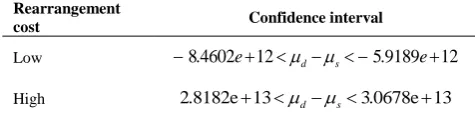
- 925120 < μdl – μs < 927000 - 905740 < μdh – μs < 955900

where μdl is the mean value of the cost function for dynamic model with low rearrangement cost, μdh is the mean value of the cost function for dynamic model with high rearrangement cost, and μs is the mean value of the cost function for static model.

The confidence interval - 925120 < μdl – μs < 927000, which is almost a symmetric interval, indicates that in the case of low rearrangement cost, the dynamic

model behaves like a static model so that the layout configuration can be easily changed from period to period. For each of the 104 test problems, the MHC of the layouts obtained by the dynamic and static approaches is computed in each period and in the whole time planning horizon. On the basis of the results, which are not shown here, the conclusions are as follows: (i) In the case of low rearrangement cost, the dynamic and static layouts have the same MHC in each period. 4. 2. Illustrative Example An example is constructed by using Problem 4 taken from Balakrishnan and Cheng [24] in such a way that the flow matrix is considered as the matrix of expectation of flow denoted by E. The matrix of variance of flow denoted by V is computed by V=E/3. This problem, which includes six facilities and five periods, is applied to each of the dynamic and static models by considering 0.75 percentile level (p).

For the dynamic model, the low, medium, and high facility rearrangement costs are set to 10, 1000, and 1,000,000 respectively.

TABLE 2. Results of the example for dynamic and static models

Model Period

No. Optimal layout

Cost per period

Total cost

Dynamic - Low

1 5 4 3 1 2 6 25066

122505 2 1 2 4 5 6 3 24752

3 4 6 1 5 2 3 23883

4 4 5 1 2 6 3 25184

5 5 4 3 2 6 1 23620

Dynamic - Medium

1 4 2 1 3 6 5 25471

125706 2 4 2 1 3 6 5 24752

3 4 2 1 5 6 3 26285

4 4 2 1 5 6 3 25578

5 2 6 1 5 4 3 23620

Dynamic - High

1 1 2 3 4 5 6 27962

144220 2 1 2 3 4 5 6 28534

3 1 2 3 4 5 6 29860

4 1 2 3 4 5 6 27206

5 1 2 3 4 5 6 30655

static

1 6 2 1 3 4 5 25066

122505 2 5 6 3 1 2 4 24752

3 5 2 3 4 6 1 23883

4 4 5 1 2 6 3 25184

Finally, the numerical example is solved by using DP algorithm and the results are shown in Table 2. Considering the first row of this table, in the case of low rearrangement cost and in period 1, for instance, facility 5 is placed in location 1, facility 4 in location 2, and so on. According to the findings, in the case of low rearrangement cost, the dynamic model behaves like static model so that the locations of facilities can be easily changed from period to period. Considering the dynamic model, for three cases of low, medium, and high rearrangement cost, the number of changes in the layout configuration over the entire planning horizon is four, three, and zero respectively. In other words, the number of changes in the layout configuration is decreased by increasing the facility rearrangement cost. As shown in Table 2 the MHC of each period is the same for the dynamic and static approaches when the rearrangement cost is low.

4. 3. Robustness Analysis In this section, the robustness of the optimal layouts obtained by each of the dynamic and static layout design models is investigated. According to Smith and Norman [25], if the decision-maker wants to design the robust layout over the interval [Pl, Pu], a robustness measure for a given layout π, i.e. R(π) can be written as Equation (29), where F1 is the inverse function for the cumulative distribution function F. The most robust layout is obtained by minimizing the R(π) [4]. Flexibility of a layout represents the ability of the layout to cope with uncertainties and fluctuations in product demands. It can be measured by using the robustness measure given in Equation (29).

 

   

 

    

 

2 2

2 2

2

l u

u l

F p F p

p p E OFV

R _{e e}

Var OFV





 

 

   

 

 

 

 

 

 _  _

_ _ 

 

 

 

(29)

To investigate the robustness of the dynamic and static layouts, 100 randomly generated test problems and four different decision maker’s defined confidence intervals are considered. The confidence intervals including [0.4 , 0.6], [0.25 , 0.5], [0.5 , 0.75], and [0.25 , 0.6] are taken from [4]. In addition, two cases of dynamic model including low and high facility rearrangement costs are regarded. As before, the values of 10 and 1,000,000 are considered as the low and high levels of the facility rearrangement cost in each period. For each of the test problems, the expectation and variance of part demands (E and V) are randomly generated with uniform distribution so that E(1000, 10000) and E(1000, 3000). Besides, both of the number of machines and the number of periods are three (M=T=3). For each of the above- mentioned confidence intervals, the 100

randomly generated test problems are applied to the aforementioned models and they are solved by using DP algorithm. The parameters used for the robustness analysis are given in Table 3. Using Equation (24), 95% confidence intervals are calculated for difference between two population means including the robustness measure of dynamic and static layouts as follows:

d s d s d s

L

_



 





U

_

The sample mean and variance and the upper and lower bounds of 95% confidence interval for μd – μs of the robustness measure values for two cases of high and low facility rearrangement costs are shown in Tables 4 and 5, respectively. The results indicate that in the case of high facility rearrangement cost, for all decision maker’s defined confidence intervals, the upper bound and the lower bound 95% confidence interval of μd – μs is positive. Therefore, the robustness of the dynamic layout is bigger than the static one. On the other hand, in the case of low facility rearrangement cost, for all decision maker’s defined confidence intervals, the upper bound and the lower bound of the 95% confidence interval of μd – μs is negative. Therefore, considering 95% confidence level, the dynamic layout has less robustness measure value than the static one.

According to Tables 4 and 5, considering the interval [0.4, 0.6], the sample mean value of the robustness measure for the two models (i.e. xd and xs), has the least value amongst the four aforementioned confidence intervals. In other words, the symmetric interval [0.4, 0.6] leads to generate the most robust layout having minimum robustness measure value.

This is due to F1(0.4) = F1(0.6) and thereby, according to Equation (29), the second term of the robustness measure (i.e. the standard deviation of the objective function) is ignored and only the first term of the robustness measure (i.e. expectation of the objective function) is minimized. In fact, decision maker’s attitude affects the robustness of the optimal layouts obtained by the two aforementioned models.

TABLE 3. Parameters of robustness analysis

Parameters Description

d

x Sample mean of robustness measure for dynamic layout

2

d

 Sample variance of robustness measure for dynamic layout

s

x Sample mean of robustness measure for static layout

2

s

 Sample variance of robustness measure for static layout

d s

L_ Lower bound of confidence interval for μd – μs

d s

TABLE 4. Robustness measure in the case of high rearrangement cost

[Pl, Pu] [0.4 , 0.6] [0.25 , 0.5] [0.5 , 0.75] [0.25 , 0.6]

d

x 3.6296

e+013

3.6321

e+013

3.6406

e+013

3.6480

e+013

2

d

 1.2107

e+021

1.9742 e+021

2.5374 e+021

4.1242 e+021

s

x 2.0653

e+012

2.3595 e+012

3.8133 e+012

5.2726 e+012

2

s

 3.3823

e+024

4.5410 e+024

1.1620 e+024

2.3050 e+024

d s

L_ 3.3870

e+013

3.3544 e+013

3.1924 e+013

3.0266 e+013

d s

U  3.4591

e+013

3.4379 e+013

3.3261 e+013

3.2148 e+013

TABLE 5. Robustness measure in the case of low rearrangement cost

[Pl , Pu] [0.4 , 0.6] [0.25 , 0.5] [0.5 , 0.75] [0.25 , 0.6]

d

x 6.0766

e+008

7.3820 e+008

1.1703 e+009

1.5959 e+009

2

d

 2.5727

e+016

3.8877 e+016

6.3052 e+016

1.4534 e+017

s

x 2.0010

e+012

2.4588

e+012

3.8630

e+012

5.2834

e+012

2

s

 3.1854

e+024

4.7572

e+024

1.2179

e+025

2.2313

e+025

d s

L_ -2.3502 e+012

-2.8856 e+012

- 4.5458 e+012

-6.2076 e+012

d s

U _ -1.6506 e+012

-2.0306 e+012

-3.1778 e+012

-4.3560 e+012

4. 4. Stability Analysis In this section, the stability of the optimal layouts obtained by each of the proposed dynamic and static models is investigated. The stability of a layout is defined as the ability of a layout to display a small sensitivity to demand changeability [20]. In other words, a layout with minimum variance of product demands is the most stable layout. Demand variability leads to variations in the materials flow between facilities, which in turn causes variations in the total cost. Therefore, the most stable layout is obtained by minimizing the variance of the total cost. In other words, the stability of a given layout π with the total cost OFV is calculated by using the stability measure S(π) given in Equation (30) so that it must be minimized for obtaining the most stable layout [20].

 





S  Var OFV (30)

To investigate the stability of the dynamic and static layouts, the 100 randomly generated test problems used in robustness analysis is solved by using the DP algorithm. The stability measure given in Equation (30) is calculated for the optimal layouts obtained by solving each of the test problems applied to the two above-mentioned models. Two cases of dynamic model containing low and high facility rearrangement costs, which are respectively set to 10 and 1,000,000 values, are considered. Using Equation (24), 95% confidence intervals are calculated for difference between two population means including the stability measure of dynamic and static layouts. Table 6 shows the 95% confidence intervals for μd – μs in the two cases of low and high rearrangement costs. In the case of low rearrangement cost, the upper bound, and the lower bound of the 95% confidence interval have negative values. It means that μd – μs is negative. As a result, there is the following relationship between the stability of the optimal layouts obtained by solving the two aforementioned models: Sd < Ss where, Sd and Ss denote the stability of dynamic and static layouts respectively. In the case of high rearrangement cost, the 95% confidence interval shows that μd – μs is positive. Therefore, Sd > Ss. In fact, the facility rearrangement cost affects the stability of both the static and the dynamic layouts.

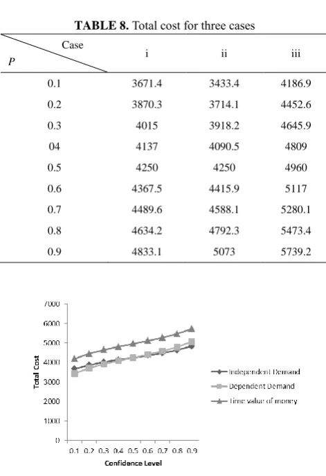
4. 5. Effect of Demands Correlation and Interest Rate on Total Cost In this section, the effect of assuming dependent part demands and time value of money (interest rate) on the total cost function of the proposed dynamic machine layout design model is investigated. To this end, a numerical example of the SDFLP with the following data is applied to each of the above-mentioned models. This problem includes two periods and three equal-sized machines placed in a line with a unit distance between each two consecutive ones. For each part, transfer batch size and movement cost are assumed to be fifty and five, respectively. Other data are given in Table 7. For the known solution [23] used in each period, the values of the objective function is calculated by considering different percentile levels (p) in the three following cases: (i) independent demands with no interest rate, (ii) dependent demands with no interest rate, (iii) independent demands with non-zero interest rate.

The results are shown in Table 8. Using the results, the cost curve for the dynamic layout design model is plotted in Figure 1.

TABLE 6. Confidence intervals for stability measure

Rearrangement

cost Confidence interval

TABLE 7. Example for analysing demands correlation and interest rate

Part Number

Variance- Covariance Matrix

Expectation of

part demand _Machinr sequence

1 2 3 Period

1

Period 2

1 10,000 640 4000 1000 1500 1→2→3

2 100 4000 10,000 15,000 2→3

3 2500 5,000 7500 1→2

Machine relocating cost = 1000 Interest rate = 10%

TABLE8. Total cost for three cases

Figure. 1. Demands correlation and time value of money

The figure indicates that a nonzero interest rate leads to increase in total cost over the range of uncertainty. As shown in Figure 1, the cost function has the same value for 0.5 percentile level (p = 0.5) for both of the independent and dependent demands because this percentile level, which is equivalent to zp= 0, leads to ignoring the second term of the objective function of the proposed dynamic layout design model given in Equation (21). According to the equation, the second term of the objective function is variance of MHC, which is a function of demands correlation. Therefore, by ignoring this term, demands correlation does not

affect the total cost of the model. Besides, the total cost is decreased for p < 0.5 (equivalent of zp < 0) and it is increased for p > 0.5 (equivalent of zp > 0) percentile levels by considering dependent demands.

5. CONCLUSION AND FUTURE RESEARCH

In this paper, to cope with the SDFLP, two QAP-based mathematical models were proposed by using the dynamic and static approaches. The proposed models were verified and validated by performing statistical, robustness and stability analyses using design of experiment and benchmark methods. The following main conclusions were obtained: (i) the dynamic layout behaves the static one in the case of low facility rearrangement cost; (ii) the robustness and stability of the dynamic layout depend on the facility rearrangement cost so that for instance, in the case of low rearrangement cost, the dynamic layout is more robust (flexible) and also more stable than the static one; (iii) however, the facility rearrangement cost does not affect the robustness and the stability of the static layout. (iv) the decision maker’s attitude about uncertainty in product demands affects the robustness of each of the dynamic and static layouts so that considering a symmetric interval leads to generate the most robust layout. (v) considering non-zero interest rate leads to increase in total cost over the range of uncertainty; (vi) considering both the dynamic and the static layouts, the effect of dependency of product demands on the total cost is a function of the decision maker’s defined percentile level so that the total cost is decreased for p < 0.5 and it is increased for p > 0.5. In addition, in the case of (p = 0.5), the total cost remains unchanged for both cases of dependent and independent demands. This research can be continued in future by considering un-equal-sized facilities and routing flexibility.

6. REFERENCES

1. Tompkins, J.A., White, J.A., Bozer, Y.A. and Tanchoco, J.M.A., "Facilities planning, John Wiley & Sons, (2010).

2. Balakrishnan, J. and Cheng, C.H., "Multi-period planning and uncertainty issues in cellular manufacturing: A review and future directions", European Journal of Operational Research, Vol. 177, No. 1, (2007), 281-309.

3. Balakrishnan, J., Jacobs, F.R. and Venkataramanan, M.A., "Solutions for the constrained dynamic facility layout problem",

European Journal of Operational Research, Vol. 57, No. 2, (1992), 280-286.

4. Kulturel-Konak, S., Smith*, A. and Norman, B., "Layout optimization considering production uncertainty and routing flexibility", International Journal of Production Research, Vol. 42, No. 21, (2004), 4475-4493.

5. Norman, B.A. and Smith, A.E., "A continuous approach to considering uncertainty in facility design", Computers & Operations Research, Vol. 33, No. 6, (2006), 1760-1775. Case

P i ii iii

0.1 3671.4 3433.4 4186.9

0.2 3870.3 3714.1 4452.6

0.3 4015 3918.2 4645.9

04 4137 4090.5 4809

0.5 4250 4250 4960

0.6 4367.5 4415.9 5117

0.7 4489.6 4588.1 5280.1

0.8 4634.2 4792.3 5473.4

6. Tavakkoli-Moghaddam, R., Javadian, N., Javadi, B. and Safaei, N., "Design of a facility layout problem in cellular manufacturing systems with stochastic demands", Applied Mathematics and Computation, Vol. 184, No. 2, (2007), 721-728.

7. Moslemipour, G. and Lee, T., "Intelligent design of a dynamic machine layout in uncertain environment of flexible manufacturing systems", Journal of Intelligent Manufacturing, Vol. 23, No. 5, (2012), 1849-1860.

8. Tavakoli-Moghadam, R., Javadi, B., Jolai, F. and Mirgorbani, S., "An efficient algorithm to inter and intra-cell layout problems in cellular manufacturing systems with stochastic demands",

International Journal Of Engineering-materials And Energy Research Center-, Vol. 19, No. 1, (2006), 67-75.

9. Palekar, U.S., Batta, R., Bosch, R.M. and Elhence, S., "Modeling uncertainties in plant layout problems", European Journal of Operational Research, Vol. 63, No. 2, (1992), 347-359.

10. Montreuil, B. and Laforge, A., "Dynamic layout design given a scenario tree of probable futures", European Journal of Operational Research, Vol. 63, No. 2, (1992), 271-286. 11. Krishnan, K.K., Cheraghi, S.H. and Nayak, C.N., "Facility

layout design for multiple production scenarios in a dynamic environment", International Journal of Industrial and Systems Engineering, Vol. 3, No. 2, (2008), 105-133.

12. Lee, T. and Moslemipour, G., Intelligent design of a flexible cell layout with maximum stability in a stochastic dynamic situation, in Trends in intelligent robotics, automation, and manufacturing. (2012), Springer.398-405.

13. Lee, T., Moslemipour, G., Ting, T. and Rilling, D., "A novel hybrid aco/sa approach to solve stochastic dynamic facility layout problem (SDFLP)", in International Conference on Intelligent Computing, Springer., (2012), 100-108.

14. Moslemipour, G., Lee, T.S. and Rilling, D., "A review of intelligent approaches for designing dynamic and robust layouts in flexible manufacturing systems", The International Journal of Advanced Manufacturing Technology, Vol. 60, No. 1-4, (2012), 11-27.

15. Tavakkoli-Moghaddam, R., Sakhaii, M. and Vatani, B., "A robust model for a dynamic cellular manufacturing system with

production planning", International Journal of Engineering, Transactions A: Basics, Vol. 27, No. 4, (2014), 587-598. 16. Hasani, A., Soltani, R. and Eskandarpour, M., "A hybrid

meta-heuristic for the dynamic layout problem with transportation system design", International Journal of Engineering-Transactions B: Applications, Vol. 28, No. 8, (2015), 1175. 17. Tavakkoli-Moghaddam, R., "A continuous plane model to

machine layout problems considering pick-up and drop-off points: An evolutionary algorithm", International Journal of Engineering Transaction B: Applications, Vol. 16, No. 1, (2003), 59-70.

18. Tayal, A. and Singh, S.P., "Integrated sa-dea-topsis-based solution approach for multi objective stochastic dynamic facility layout problem", International Journal of Business and Systems Research, Vol. 11, No. 1-2, (2017), 82-100.

19. Rezazadeh, H., Ghazanfari, M., Saidi-Mehrabad, M. and Sadjadi, S.J., "An extended discrete particle swarm optimization algorithm for the dynamic facility layout problem", Journal of Zhejiang University-Science A, Vol. 10, No. 4, (2009), 520-529.

20. Ripon, K., Glette, K., Hovin, M. and Torresen, J., "Dynamic facility layout problem under uncertainty: A pareto-optimality based multi-objective evolutionary approach", Open Computer Science, Vol. 1, No. 4, (2011), 375-386.

21. Vitayasak, S., Pongcharoen, P. and Hicks, C., "A tool for solving stochastic dynamic facility layout problems with stochastic demand using either a genetic algorithm or modified backtracking search algorithm", International Journal of Production Economics, (2016).

22. Braglia, M., Zanoni, S. and Zavanella, L., "Robust versus stable layout design in stochastic environments", Production planning & control, Vol. 16, No. 1, (2005), 71-80.

23. Freund, J., "Mathematical statistics" (1992), Prentice-Hall.

24. Balakrishnan, J. and Cheng, C.H., "Genetic search and the dynamic layout problem", Computers & Operations Research, Vol. 27, No. 6, (2000), 587-593.

Performance Analysis of Dynamic and Static Facility Layouts in a Stochastic

Environment

G. Moslemipoura_{, R. Tavakkoli-Moghaddam}b,c

a _{Department of Industrial Engineering, Payame Noor University, Iran}

b _{School of Industrial Engineering, South Tehran Branch, Islamic Azad University, Tehran, Iran} c _{School of Industrial Engineering, College of Engineering, University of Tehran, Tehran, Iran}

P A P E R I N F O

Paper history: Received 28 January 2017

Received in revised form 25 February 2017 Accepted 10 March 2017

Keywords:

Dynamic Facility Layout Quadratic Assignment Uncertainty Dynamic Programming

ديكچ ه

هرود دنچ( ایوپ هلئسم لح یارب ،هلاقم نیا رد هلئسم رب ینتبم دیدج یضایر لدم ود ،تلایهست نامدیچ یفداصت و )یا

یم هئارا اتسیا و ایوپ یاهدرکیور زا کی ره اب رظانتم و یمود هجرد صیصخت لدم نیا رد .دندرگ

نتفرگرظن رد رب هولاع ،اه

شرگن و لوپ ینامز شزرا اب هتسباو یفداصت ییاهریغتم تلاوصحم یاضاقت ،تیعطق مدع صوصخ رد هدنریگ میمصت

یم ضرف لامرن عیزوت هنوگ هب دنوش

روط هب اهنآ سنایاووک و سنایراو ،نیگنایم هک یا یفداصت

هرود هب ینامز هرود کی زا

-یم رییغت رگید یا دننک

لدم رابتعا و یتسرد . لیلحت ماجنا اب ،یداهنشیپ یاه

ه زا هدافتسا اب یرادیاپ و یراوتسا ،یرامآ یا

شور یم یسررب درادناتسا لئاسم لح و شیامزآ یحارط یاه وش

لدم نیا لح یارب .دن هک ایوپ یزیر همانرب متیروگلا زا ،اه

یم هدافتسا تسا هدش یسیون دک بلتم تاروتسد طسوت وش

مهم .د جیاتن نیرت قیقحت نیا ( :زا دنترابع 1

نییاپ تلاح رد )

( .تساتسیا نامدیچ هباشم یراتفر یاراد ایوپ نامدیچ ،نامدیچ رییغت هنیزه ندوب 2

یراوتسا نازیم ،اتسیا نامدیچ فلاخرب )

( .دنراد نامدیچ رییغت هنیزه هب یگتسب ایوپ نامدیچ یرادیاپ و 3

نازیم رب تیعطق مدع صوصخ رد هدنریگ میمصت شرگن )

نامدیچ زا کیره یراوتسا تسیا و ایوپ یاه

( .تسا رثؤم ا 4

هنیزه شیازفا هب رجنم ،رفص ریغ یلوپ هرهب خرن نتفرگ رظن رد )

یم تیعطق مدع هنماد رساترس رد لک ( .ددرگ

5 یور تلاوصحم یاضاقت یگتسباو ریثأت ،اتسیا و ایوپ نامدیچ ود ره یارب )