Issues
ISSN: 2146-4138
available at http: www.econjournals.com
International Journal of Economics and Financial Issues, 2016, 6(4), 1338-1343.
Changes in the Unconditional Variance and Autoregressive
Conditional Heteroscedasticity
Amado Peiró*
Universitat de València, Valencia, Spain. *Email: [email protected]
ABSTRACT
This paper argues that a simple white noise process with one jump in its unconditional variance may give rise to the presence of autoregressive conditional heteroscedasticity (ARCH) effects, and, surprisingly, this may occur in determinate circumstances even when the jump is very brief. Though ARCH effects are not denied, this evidence, together with some empirical results obtained from Standard & Poor’s 500 returns, allows one to question whether they are a general and regular property of so many economic and financial series.
Keywords: Autoregressive Conditional Heteroscedasticity, Stock Returns, Unconditional Variance JEL Classification: G12
1. INTRODUCTION
More than three decades ago Engle (1982) introduced a new class of stochastic processes called autoregressive conditional heteroscedasticity (ARCH) models and used them to estimate
the variance of UK inflation. This seminal contribution generated
huge interest and very soon different types of ARCH models were proposed: GARCH, integrated GARCH (IGARCH), exponential GARCH or ARCH-M, to name just a few from the many models
which constitute, in Engle’s (2002) own words, a continually
amazing soup of volatility models. One of the main reasons that underlie this huge interest in ARCH models is the profusion of economic series that seem to present ARCH effects. This is
especially true with regard to financial series; returns from different
assets and from different markets seem to exhibit ARCH effects almost universally. Given this profusion and the fact that volatility
is a key variable in many financial models, the analysis of ARCH
has received great attention from many researchers.
Among these many researchers, very few have studied the consequences of outliers or breaks in volatility in ARCH models and the potential spurious or misleading conclusions that may follow. Already Diebold (1986) pointed out that integrated variance models could correspond to “stationary GARCH movements within regimes, with an unconditional “jump”
occurring between regimes.” When analyzing the US long-run interest rate, Franses (1995) showed that a one-time variance change spuriously suggested that this variable could be described with an IGARCH process, and, moreover, the sub-periods did
not show characteristics of ARCH. Franses et al. (2004) show
that patches of additive outliers can have substantial effects on
tests for ARCH. More recently, Hillebrand (2005), Rapach and Strauss (2008), Xu and Phillips (2008) or Gregory and Reeves (2010) have drawn the attention to the fact that outliers, structural
breaks or simple changes in the unconditional variance may
lead to parameter bias or severe model misspecifications. More specifically, they argue that neglecting or ignoring these features
yield severe upward biases in the estimation of the persistence of GARCH models.
Though most research on this topic highlights its effect on persistence, the impact of breaks or jumps could be much more important. Not only the persistence, but even the mere existence of ARCH or its magnitude could be due to these changes, even when they are limited to very few variables in the process. This paper aims to explore the possibility that the magnitude of ARCH effects or the plain existence of ARCH, according to usual tests,
in so many financial and economic series may originate from
a white noise process with one jump in its conditional variance and studies, via Monte Carlo simulations, the existence of ARCH effects in these processes. In Section 3, ARCH is tested in Standard
& Poor’s (SP) 500 returns with different samples and with different
return frequencies, and the robustness and sensitivity of the ARCH effects is casually examined. Finally, Section 4 summarizes the main results and conclusions.
2. SOME SIMULATIONS
Let us consider the following process:(
1) (
1)
(
1)
, 1, 2, , , 1, 2, ,
2 2 2
− + +
= = … + + …
t t
T T T
Y t T
(
1)
(
1)
(
1)
, 1, 2, ,
2 2 2
− − +
= = + + …
t t
T T T
Y t
(1)
Where, εt is i.i.d. N(0,1), 0 < λ < 1, and γ > 1. For notational
convenience, and without loss of generality, let us also suppose
that λT is even (odd) if T is even (odd). This process is composed by T variables which follow a standard normal distribution with
the exception of the λT central variables which follow a normal
distribution with expectation 0 and variance γ2. Thus, for example,
if T = 100, λ = 0.04 and γ = 2, the following process is obtained:
Yt = εt, t = 1, 2,…,48, 53, 54,…,100
Yt = 2εt, t = 49, 50, 51, 52
With εt i.i.d. N(0,1). That is, the process is formed by 100 variables,
all of which are N(0,1) excepting the 4 central variables which
are N(0,22).
Obviously, the process {Yt} is not i.i.d. It is stationary in the mean, but non-stationary in the variance. However, the process formed
exclusively by the first (or by the last) (1−λ)T/2 variables is a simple i.i.d. N(0,1) process, and the process formed by the λT
central variables is a simple i.i.d. N(0,γ2) process. This process
can be regarded as a white noise N(0,1) process with an episode
of higher variability at the middle. By construction this process
presents ARCH. However, for low values of λ, the ARCH is due to
the existence of a few consecutive variables with a higher variance surrounded by variables with a lower variance. It is not a general property of the whole process. Neither the process formed only
by the first (1−λ)T/2 variables, nor the process formed only by the
last (1−λ)T/2 variables, nor the process formed exclusively by the
λT central variables presents ARCH. But the whole process does present ARCH because it has been built in such a way that the variables with different variances are grouped apart.
This process is similar to a discrete mixture of (two) normal distributions. These models were proposed by Christie (1983) or Kon (1984) to analyse the unconditional distribution of stock returns. However, there is a fundamental difference. While in, for example, Kon (1984) the returns are drawn randomly from either of the two normal distributions, in (1) the variables drawn
from the two distributions are grouped in a deterministic way. The variables with a higher variance are consecutive in the middle of the process, and not scattered randomly. On the other hand, it is
evident that this process fulfills the famous observation made by
Mandelbrot (1963) and frequently invoked in ARCH literature: “Large changes tend to be followed by large changes–of either sign–and small changes tend to be followed by small changes.”
It would be interesting to test for ARCH in process (1). The existence of ARCH effects in a series is usually tested by using the Lagrange multiplier (LM) test of Engle (1982). Consequently, to test for ARCH, the following regressions will be carried out:
Yt Y u
i p
i t i t
2
1 2
= + +
= −
∑
α β
Where, α, β1, β2,…,βp are parameters, and ut is the error term. The statistics TR2, where T is the sample size and R2 is the
coefficient of determination, will be computed for p = 1, 5 and 10. These statistics will be denoted by LM(1), LM(5) and LM(10),
respectively. Under the null hypothesis of absence of ARCH
effects, β1 = β2 = ... = βp = 0, these statistics follow asymptotically a χ2 distribution with p degrees of freedom.
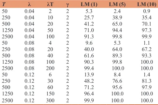
In order to analyze the possible presence and intensity of ARCH
effects in these processes, 10,000 realizations were simulated
for different sets of values of T (50, 250, 500, 1,250 and 2500), λ (4%, 8% and 12%), and with γ equal to 2. LM tests were run for
these simulated processes. Table 1 presents the relative frequency
of rejections of the null of absence of ARCH at the 5% significance
level. Several conclusions arise from Table 1. Firstly, for each value of T, the probability of concluding the existence of ARCH
increases with the proportion λ. Secondly, for each value of λ, the
empirical probabilities of rejection increase clearly with the sample size. For T = 50 and λ = 0.04 these probabilities are rather low, but
they increase monotonically with the sample size. The same occurs
for λ = 0.08 or for λ = 0.12. As a consequence of this increase, they
approach to unity for large sample sizes. In fact, they are virtually equal to unity in many cases for T = 1250 or T = 2500. This implies that with at least 4% of central variables whose standard deviation
Table 1: Rejections in LM tests with simulated processes
T λ λT γ LM (1) LM (5) LM (10)
50 0.04 2 2 5.3 2.4 0.9
250 0.04 10 2 25.7 38.9 35.4
500 0.04 20 2 41.2 65.0 70.1
1250 0.04 50 2 71.0 94.4 97.3
2500 0.04 100 2 91.3 99.8 99.9
50 0.08 4 2 9.6 5.3 1.1
250 0.08 20 2 40.0 64.0 67.2
500 0.08 40 2 61.6 89.3 93.3
1250 0.08 100 2 90.3 99.8 100.0
2500 0.08 200 2 99.4 100.0 100.0
50 0.12 6 2 13.9 8.4 1.4
250 0.12 30 2 48.2 76.6 81.3
500 0.12 60 2 71.2 95.6 97.9
1250 0.12 150 2 96.4 100.0 100.0
2500 0.12 300 2 99.9 100.0 100.0
is the double of that of the other variables, one may expect to find
ARCH with a very high probability for these sample sizes. In
terms of financial returns, this would mean that in 5 years of daily
returns (T = 1250, approximately) with two central months whose daily returns (λT = 50, approximately) had a standard deviation
that was the double of that of the others, ARCH would follow in
94.4% of cases, according to the LM(5) test.
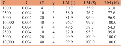
The previous proportions of central variables with a higher
variability (4%, 8% or 12%) are arbitrary. They have been chosen so that λT is equal to, at least, a few variables with higher standard deviation. It would be interesting to study the effects of lower
proportions. Therefore, proportions as low as 4‰, 8‰, or 2% will
be considered, but the sample sizes must now be high enough so
that λT must yield at least a few central variables with a higher standard deviation. Table 2 presents the results obtained with these new values for T and λ. Once again, the rates of rejections increase when λ increases, but, for these large sample sizes, they all are well above the significance level of 5%, even for a proportion as low as λ = 0.004. Thus, for example, for T = 5000 and λ = 0.004, the probability of finding ARCH is 43.7% with the LM(10) test. In other words, this means a probability of 43.7% of finding ARCH with 20 years of daily returns (T = 5000, approximately) with a
given variability, with the exception of those in the central month
(λT = 20, approximately) whose variability is twice of the others.
Finally, it is also interesting to analyze the effects of γ on the rates of rejection. γ = 2 is probably a moderate ratio between the
standard deviation of central variables and the standard deviation
of the non-central variables. Higher values such as γ = 3 or γ
= 4 suppose a higher ratio which could be more plausible to give account of different episodes of higher variability in many
processes, and in particular in many financial markets. Table 3
shows the results of LM tests for these values. The empirical
rejection rates increase strongly when γ increases. For T = 2500 and λ = 0.004, the probabilities of finding ARCH with the LM(5) test, for example, go from 24.0% for γ = 2, to 76.7% for γ = 3, and to 95.3% for γ = 4. From the perspective of financial markets,
this last value would imply that the probability of concluding
ARCH with 10 years of daily returns that include only 2 weeks of “abnormal” daily returns is 95.3%.
Taking into account the values of the preceding simulations, the conclusions are clear and sharp. They show that: (i) Evidence of ARCH is not found or is hardly found for determinate combinations of T, λ, γ; (ii) the probability of finding ARCH
increases monotonically with T, λ, γ; (iii) processes with high
values for T and/or γ present ARCH effects with a very high probability, even for very low values of λ. By construction, process (1) presents ARCH; therefore, it should not be surprising
rejections of the null of no ARCH. What is very surprising is the high proportion of rejections with so few variables with a higher variance. Only a few variables drive the results obtained with very large samples. Though ARCH does exist in all these cases, it is not a general or regular property of the process. Rather, ARCH is due to the existence of two different regimes involved in process
(1) which are reflected in each of the two equations that compose
this process. Instead of thinking this process as a regular process
with systematic ARCH all over time, it would be wiser to consider this process as formed by two different regimes. Each of them does not present ARCH, but the co-existence of both regimes does imply the manifestation of ARCH effects1.
One could question if these results are due to the fact that the group of variables with higher variance is located exactly in the middle of the series. Simulations (not shown but available upon request) with this group of variables located in different intervals of the sample showed very similar results. Analogously, one could question if the results are due to the fact that the variables with higher variance are consecutive in one single group. Once again, new simulations showed that similar results would also apply (with
the appropriate modifications) to other hypothetical processes
where the variables with higher variability were scattered in a few groups. For example, the results for T = 5000 and λ = 0.004 are very similar when arranging the λT variables with higher variance
in one single group of 20 variables, than when arranging them in two separate groups of 10 variables each, or when they are
arranged in four separate groups of 5 variables each. Of course, in the limit, when these variables are scattered randomly, ARCH evidence disappears.
Therefore, the preceding simulations show that a long series with a short episode of higher variability will present ARCH effects with a high probability. Evidently, these results do not imply that
1 In addition, it is interesting to note that these simulated series systematically present excess kurtosis or high autocorrelations of absolute values, among
other stylized facts of asset returns (see, for example, Cont, 2001).
Table 2: Rejections in LM tests with simulated processes
T λ λT γ LM (1) LM (5) LM (10)
1000 0.004 4 2 10.5 10.5 9.4
2500 0.004 10 2 16.5 24.0 22.9
5000 0.004 20 2 24.0 39.8 43.7
10,000 0.004 40 2 35.8 62.1 70.2
1000 0.008 8 2 18.1 25.6 22.8
2500 0.008 20 2 31.1 50.6 54.8
5000 0.008 40 2 47.6 75.4 81.7
10,000 0.008 80 2 70.2 94.7 97.3
1000 0.02 20 2 38.8 61.8 66.7
2500 0.02 50 2 65.9 91.4 98.2
5000 0.02 100 2 88.3 99.5 99.9
10,000 0.02 200 2 98.8 100.0 100.0
Percentages of rejections at the 5% significance level in LM tests for ARCH in 10,000 simulations of processes (1) for different values of T and λ. LM: Lagrange multiplier, ARCH: Autoregressive conditional heteroscedasticity
Table 3: Rejections in LM tests with simulated processes
T λ λT γ LM (1) LM (5) LM (10)
1000 0.004 4 3 30.7 35.9 31.8
2500 0.004 10 3 58.0 76.7 77.6
5000 0.004 20 3 81.9 96.0 96.9
10,000 0.004 40 3 96.7 99.9 100.0
1000 0.004 4 4 49.5 58.3 54.3
2500 0.004 10 4 82.0 95.3 95.8
5000 0.004 20 4 99.9 100.0 100.0
10,000 0.004 40 4 99.9 100.0 100.0
this is the only fact that explains the existence of ARCH effects
in so many series or that it is the main factor; it could be just a
contributing factor of limited importance or a determining factor only in some cases. The relevant question, therefore, is whether these limited episodes of higher variability play an important role in the ARCH evidence reported in so many actual economic or
financial series. A clear-cut answer to this question is difficult, but
two pieces of evidence suggest that very frequently the answer
may be affirmative. First, if it is the case, longer series will present
ARCH evidence much more often than shorter ones, as episodes of higher variability are much more probable in long series than in short series. Second, if it is the case, ARCH detection relies on a few observations and small changes in these observations would
significantly alter the results in ARCH tests. In the next section
some evidence on these two points will be reported.
3. EVIDENCE ON SP’S 500 RETURNS
ARCH evidence has been reported in many different series. Inwhat follows the SP’s 500 Composite index will be considered from 1950 to 2009. Though this is the only series studied in this article, it is a financial series of the maximum importance with a
large coverage of US equities and a rather long time span. Besides, this series has very often been used in ARCH modeling. Daily
closing values were available from January 3, 1950 to December 31, 2009. After excluding those days when stock markets were closed, daily returns were obtained by logarithmic differences;
that is by Rt = log(It/It−1), where Rt is the return for day t, It is the daily index for the same day and It−1 is the daily index for the preceding day. Thus, the series of daily returns is composed
by 15,096 observations. Weekly returns have been computed by
subtracting to the logarithm of the value of the index in the last trading day (usually Friday) of a certain week the logarithm of the value of the index in the last trading day (usually Friday) of the
preceding week. In this way, a series of 3130 weekly returns has
been obtained. Monthly returns have been obtained by subtracting to the logarithm of the value of the index in the last trading day of the month the logarithm of the value of the index in the last trading day of the preceding month. The series of monthly returns
is composed by 720 observations.
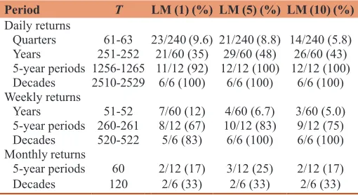
As in the preceding section, the existence of ARCH effects in a series will be tested by using the statistics LM(1), LM(5) and
LM(10). With these statistics and with daily returns ARCH is tested in the 240 different quarters comprised between the first quarter of 1950 and the fourth quarter of 2009. A typical quarter
includes between 61 and 63 daily returns. Table 4 shows the
proportion of rejections at the 5% significance level. In 23 out of the 240 quarters the null of no ARCH was rejected at the 5% level
when using the statistic LM(1), in 21 with LM(5), and in 14 with
LM(10). It is surprising that, though ARCH is considered to be very usual among financial series, only a few quarters (<10%) present
evidence of these effects. Moreover, as the probability of a Type I
error is 5%, the rejections do not exceed by a large amount what
is to be expected in absence of ARCH effects. The proportion of
rejections increases significantly when the same tests are applied with daily returns to each of the 60 years comprised between 1950 and 2009. A typical year includes between 251 and 252 daily
returns. Now, in the 60 years, the null hypothesis of absence of
ARCH is rejected in 21 of them with the LM(1) statistic, in 29
with the LM(5) statistic and in 26 with the LM(10) statistic; that
is, the rates of rejections are comprised between one third and one half, which mean that ARCH effects are frequent though not pervasive. With longer sample periods, such as periods of 5 years or decades, the evidence in favor of ARCH in daily returns
becomes overwhelming. A period of 5 years includes about 1260 daily returns, and a decade about 2520 daily returns. In all but
one 5-year period the null hypothesis of nonexistence of ARCH is rejected with the different LM statistics, and in all decades this hypothesis is always rejected.
Let us now consider weekly returns instead of daily returns. As the number of weeks comprised in a quarter is relatively low (about 13), it does not seem reasonable to analyze the existence of ARCH effects in a quarter by using weekly returns. Instead, the shortest time span will now be a year, which typically comprises between 51 and 52 weekly returns. With the same LM tests, Table 4
shows the proportion of rejections with weekly returns at the 5% significance level in the 60 years comprised between 1950 and 2009. These proportions are very low again. Indeed, when the LM(10)
statistic is used, the proportion of rejections is exactly equal to the
size of the test (5%). With 5-year periods or decades the results are rather different; between 67% and 83% of the 5-year periods and
almost all decades present evidence of ARCH with the different LM tests. Finally, let us consider monthly returns. Analogously to the limitation exposed above, it does not seem reasonable to conduct ARCH tests in a given year with only 12 observations. Accordingly, Table 4 only shows the results for 5-year periods and decades. ARCH is found in between one sixth and one fourth of the 12 5-year periods, and in one third of the six decades.
All this evidence suggests that ARCH may not be a ubiquitous feature of stock index returns when considering moderate sample sizes such as quarters or years of daily returns, years of weekly returns, or 5-year periods or decades of monthly returns. On the contrary, with larger sample sizes the detection of ARCH effects is
an almost universal rule. These facts reflect that ARCH detection
occurs much more frequently with longer series, where episodes
Table 4: Rejections in LM tests with SP returns
Period T LM (1) (%) LM (5) (%) LM (10) (%)
Daily returns
Quarters 61-63 23/240 (9.6) 21/240 (8.8) 14/240 (5.8) Years 251-252 21/60 (35) 29/60 (48) 26/60 (43) 5-year periods 1256-1265 11/12 (92) 12/12 (100) 12/12 (100) Decades 2510-2529 6/6 (100) 6/6 (100) 6/6 (100) Weekly returns
Years 51-52 7/60 (12) 4/60 (6.7) 3/60 (5.0) 5-year periods 260-261 8/12 (67) 10/12 (83) 9/12 (75) Decades 520-522 5/6 (83) 6/6 (100) 6/6 (100) Monthly returns
5-year periods 60 2/12 (17) 3/12 (25) 2/12 (17)
Decades 120 2/6 (33) 2/6 (33) 2/6 (33)
of higher variability are much more probable. For example, in process (1), if T = 1000 and λ = 0.02, the probability that a
sample of size N will contain all the observations coming from
the variables with higher variance will be 4.4% for N = 60, 30.8%
for N = 250, and 96.0% for N = 500 In temporal terms, this means
that in 4 years of daily returns (T ≈ 1000) with the daily returns
in the central month (λT ≈ 20) having a higher variability, the
probability that a quarter (N ≈ 60) will contain this central month is about 4.4%, for 1 year (N ≈ 250) the probability is 30.8%, and
for 2 years (N ≈ 500) it is 96.0%.
Nevertheless, these longer series that cover a large span of time include more returns of the same frequency than shorter series, and the power of the LM tests will increase with the sample size.
Therefore these two factors are inextricably linked; longer series
will contain more observations (and, consequently, statistical tests will be more powerful) and will have a higher probability of changes in variability (and, according to the simulations of the preceding section, ARCH will follow). To disentangle both
elements would require a specific study, but, in any case, the
preceding evidence shows that short or moderate samples with reasonable sizes, such as those formed by one quarter or by 1 year of daily returns, do not present ARCH evidence systematically, while longer samples do.
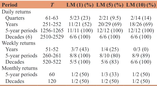
If ARCH in a process is due to a few variables with higher variability, small changes in these variables would alter
significantly the results of ARCH tests. On the contrary, if
ARCH is a general property of the process, not due to a few variables, small changes in these variables would not have an important effect on ARCH results. To cast some light on this point, ARCH tests were repeated in those samples which present ARCH evidence, according to the results shown in Table 4, but replacing the most extreme squared return by the mean in the sample. Thus, for example, in those quarters with ARCH evidence for daily returns, the most extreme squared return was replaced by the mean of the squared returns in the same quarter, and the LM tests were run again. Table 5 shows
that ARCH effects were found in only 5 out of the 23 quarters with previous evidence of ARCH, in 2 of the 21 quarters and in 2 of the 14 quarters, according to the different LM statistics. That is, ARCH evidence disappeared in 18 out of the 23 quarters
whose LM(1) statistics were significant. It also disappeared in almost all (19) quarters whose LM(5) statistics were significant, and in 12 out of the 14 quarters with a significant LM(10)
statistic. Though these extreme returns are probably among
the most influential in each quarter, it is surprising to see
how heavily the autocorrelation structure of squared returns depends on one single value in a sample typically formed by
60-65 observations. Analogously, when taking into account
years of daily returns, the most extreme squared return in each year with ARCH effects has been replaced by the mean of the squared returns in the same year. The number of rejections also decreases strongly, but not as drastically as with quarterly
samples. ARCH evidence disappears in 10 out of the 21 years
that presented previous evidence according to the LM(1) statistic, in 9 out of the 29 years with the LM(5) tests, and in
8 out of the 26 years with the LM(10) statistic. These results
indicate the sensitivity of these tests, as they are affected by
only one observation (maybe the most influential) out of some 250 observations in each year. However, the same casual study
of robustness with longer periods of daily returns show that, in all the 5-year periods and decades with ARCH evidence, the results did not change when replacing the most extreme squared return by the mean squared return, but this is hardly
surprising as only one out of about 1250 or 2500 observations
had been changed.
The same informal tests of robustness with years of weekly returns suggest that ARCH is not a robust feature as the evidence disappeared in more than half of the years (4 out of 7 and 3 out of 4, according to the LM(1), LM(5) statistics, respectively) and
in all the years (3 out of 3), according to the LM(10) statistic.
Nevertheless, it must be admitted that, in spite of these drastic changes in years of weekly returns, the ARCH evidence disappears much less with longer periods of weekly returns such as 5-year periods or decades. Finally, the ARCH evidence with monthly returns seems to be also very sensitive, as it disappears in more than the half of the 5-year periods, and in half of the decades. When the results in Tables 4 and 5 are taken together, one comes to the conclusion that ARCH is a common phenomenon of long periods with large samples, such as 5-year periods or decades of daily or weekly returns. With shorter periods or with smaller samples, ARCH is not a prevalent and robust feature. It is neither prevalent nor robust with quarters or years of daily or weekly returns, or with 5-year periods or decades of monthly returns. In fact, robust ARCH evidence is almost absent in quarters of daily returns, in years of weekly returns and in 5-year periods of monthly returns. All these results point to the possibility that short episodes of higher variance could be behind many series that present ARCH evidence.
Finally, it is important to stress that process (1) does not pretend to
be a “model” for any economic or financial series. It simply intends
to illustrate the effects of a break in the unconditional variance of a very simple process on the existence of ARCH effects. It is
Table 5: Rejections in LM tests with SP returns in periods with previous ARCH evidence after replacing the most extreme return
Period T LM (1) (%) LM (5) (%) LM (10) (%)
Daily returns
Quarters 61-63 5/23 (23) 2/21 (9.5) 2/14 (14) Years 251-252 11/21 (52) 20/29 (69) 18/26 (69) 5-year periods 1256-1265 11/11 (100) 12/12 (100) 12/12 (100) Decades (6) 2510-2529 6/6 (100) 6/6 (100) 6/6 (100) Weekly returns
Years 51-52 3/7 (43) 1/4 (25) 0/3 (0)
5-year periods 260-261 8/8 (100) 8/10 (80) 8/9 (89) Decades 520-522 5/5 (100) 5/6 (83) 6/6 (100) Monthly returns
5-year periods 60 1/2 (50) 1/3 (33) 1/2 (50)
Decades 120 1/2 (50) 1/2 (50) 1/2 (50)
also important to stress that only one financial series has been
examined. Much more work is needed and further research should consider different types of jumps in different processes as well as examine other series in the light of the evidence reported here.
4. CONCLUSIONS
The study of the effects of jumps or breaks in unconditional volatility on ARCH models has usually been limited to the effects on persistence of GARCH models, However, the literature is very sparse or non-existent on a much more important topic such as their effects on the effective existence of ARCH in time series as an overall, regular and systematic property of these series.
In order to cast some light on this point, two arguments are presented in this paper. First, a simple white noise with a jump in its unconditional variance is taken into account and different simulations with this process show that ARCH follows very frequently in conventional tests even with short episodes of higher
variance. Second, SP’s 500 returns for different sample periods and
different frequencies are examined. The results obtained show that ARCH is not a usual feature of short or moderate periods or samples and, moreover, ARCH evidence does not seem to be very robust in many cases. All these arguments allow one to question whether
ARCH effects are a general property of economic and financial
series and, conversely, to wonder whether short jumps in the unconditional variability may play an important role in these effects. Of course, this does not question the effective existence of ARCH
as a regular feature of many economic and financial series, but it
draws attention to the fact that in some cases the results obtained may be contaminated by brief unconditional variance jumps.
REFERENCES
Christie, A. (1983), On Information Arrival and Hypothesis Testing in Event Studies. Working Paper, University of Rochester.
Cont, R. (2001), Empirical properties of asset returns: Stylized facts and statistical issues. Quantitative Finance, 1, 223-236.
Diebold, F.X. (1986), Modeling the persistence of conditional variances: A comment. Econometric Reviews, 5, 51-56.
Engle, R. (1982), Autoregressive conditional heteroscedasticity with estimates of the variance of United Kingdom inflation. Econometrica, 50, 987-1007.
Engle, R. (2002), New frontiers for ARCH models. Journal of Applied Econometrics, 17, 425-446.
Franses, P.H., Van Dijk, D., Lucas, A. (2004), Short patches of outliers, ARCH and volatility modelling. Applied Financial Economics, 14, 221-231.
Franses, P.H. (1995), IGARCH and variance change in the US long-run interest rate. Applied Economics Letters, 2, 113-114.
Gregory, A.W., Reeves, J.J. (2010), Estimation and inference in ARCH models in the presence of outliers. Journal of Financial Econometrics, 8, 547-569.
Hillebrand, E. (2005), Neglecting parameter changes in GARCH models. Journal of Econometrics, 129, 121-138.
Kon, S.J. (1984), Models of stock returns – A comparison. Journal of Finance, 39, 147-165.
Mandelbrot, B. (1963), The variation of certain speculative prices. Journal `of Business, 36, 394-419.
Rapach, D.E., Strauss, J.K. (2008), Structural breaks and GARCH models of exchange rate volatitlity. Journal of Applied Econometrics, 23, 65-90.